Induced Redundancy based Lossy Data Compression Algorithm

Induced Redundancy based Lossy Data

Compression Algorithm

Kayiram Kavitha

Lecturer, Dept. of CS & IS,

BITS-Pilani, Hyderabad Campus,

Hyderabad, India.

Dhruv Sharma

Student, Dept. of CS & IS,

BITS-Pilani, Hyderabad Campus,

Hyderabad, India

.

Rahul Surana

Student, Dept. of CS & IS,

BITS-Pilani, Hyderabad Campus,

Hyderabad, India.

R. Gururaj,

Dept. of CS & IS, BITS-Pilani, Hyderabad Campus,

Hyderabad, India.

ABSTRACT

A Wireless Sensor Network (WSN) is an increasingly important mechanism for enabling continuous monitoring and sensing of physical variables like temperature, humidity etc. The tiny sensor nodes are powered by low capacity batteries. As the WSNs are usually deployed in remote areas, battery replacement becomes difficult. To minimize the power consumption in WSN, the data compression schemes play a vital role. If applied appropriately, these data compression schemes can result in drastic increase in the lifetime of the network. In this paper, we present a scheme called Induced Redundancy based Lossy Data Compression Algorithm, (IR-LDCA), which is best suited for WSNs that sense data with higher correlation. Our algorithm induces certain amount of redundancy into the data set to achieve more effective data compression and also gives the user a flexibility to control the compression ratio and loss of data. Simulation results prove the effectiveness of the proposed scheme over the existing ones.

General Terms

Data Compression, Optimization, Redundancy.

Keywords

WSN, correlated data, lossy compression, IR-LDCA.

1.

INTRODUCTION

A Wireless Sensor Network (WSN) [1] comprises of several sensor nodes communicating with each other to perform a common task i.e., to transfer the sensed data to the station. In WSN, one of the nodes is designated as the base-station that connects the WSN with the outside world. Each sensor node predominantly consists of a processor, sensor and a radio communication module powered by a battery. The sensor node makes use of radio communication module for transmitting data to the base-station (possibly via other intermediate nodes). The radio communication module is a dominant consumer of energy. Hence, efficient management of battery power is desired in the design of any WSN. The replacement or recharge of batteries is impossible as their deployment is in remote geographic locations, and sometimes with extreme weather conditions. Thus, it is desirable to reduce the consumption of energy in order to enhance the lifetime of the network. It is desirable to incorporate energy efficient schemes in various operations of the WSN like- storage, data transmission, computations etc. Some of the important techniques that are adopted for achieving energy efficiency are- duty cycling [2], aggregation [3], and in-network processing [4]. Duty cycling is a scheme, according

to which a sensor node switches between active and sleep modes. During the active mode, it will be sensing, computing or transmitting data. This scheme switches the sensor to sleep mode when there is no sensing or transmission activity in the network. As the node is shut down temporarily, the node would be operating in power saving mode with minimal consumption. This ensures optimal power utilization in the network. The aggregation scheme in WSN is the one where every intermediate node performs combination of data received from other nodes (intending to send data to station), and transmit the combined data towards the base-station, so as to derive fewer data items than what it has received, to be forwarded to the next node on the way to the base-station. The aggregation may involve functions such as min, max, average, count, and sum. The duplicate suppression involves forwarding distinct data items, while discarding the duplicate ones. This results in fewer data items for transmission. The other aggregate functions mentioned above, when applied on the data stream will always result in single value. Thus, this scheme results in reduced power consumption during data routing due to reduced number of packets. The in-network processing scheme is to reduce the quantity of data transmitted, by applying data compression schemes [5]. Since the proposed work in this paper is closely related to data compression, the in-network processing scheme is elaborated in the following paragraph.

at the receiving end i.e., without any loss in the precision of the data. But this hinders achieving higher compression ratios. With lossy compression, some degree of information loss, presented in terms of RMS error (Root Mean Square error), is present. In order to achieve higher compression ratio, the lossy compression scheme exploits the redundancy in sensor data. Thus, for WSN applications which doesn’t require high precision, lossy compression techniques are more preferable. In this paper, a new lossy compression scheme called as Induced Redundancy based Lossy Data Compression Algorithm (IR-LDCA) is proposed to compress the data under transmission in the network. The proposed algorithm provides means to control the compression ratio and loss of data after compression. The performance evaluation experiments conducted for comparing the effectiveness of the proposed IR-LDCA against the existing lossy data compression scheme K-RLE [8] have shown promising results.

The rest of the paper is organized as follows. The related work is discussed in Section 2, and the proposed scheme with algorithms and illustrations is described in Section 3. Section 4 shows the simulation setup and experimental results. Finally, the conclusion is presented in Section 5.

2.

RELATED WORK

There has been a significant amount of work done on data compression in WSN. As mentioned in Section 1, data compression schemes employed in WSN can be classified into two. The first one being the lossless data compression and the second is the lossy data compression technique. In this paper a lossy data compression scheme optimized for WSN data is proposed.

2.1 Lossless Data Compression schemes

The Lossless algorithms, as the name indicates compresses data without any loss of data. Hence, applications requiring higher precision adopt these schemes. It is obvious that higher compression ratios cannot be achieved with higher precision. The Modified Adaptive Huffman coding algorithm [9] is a lossless data compression algorithm. The algorithm uses a tree approach with leaves representing sets of symbols with the same frequency. The number of levels in the tree is reduced to enhance the performance of the scheme and bringing the maximum possible elements to the top of the tree. This algorithm uses the above mentioned tree to assign a smaller bit sequence representation to the symbols with higher frequencies and similarly a larger bit sequence for the symbols with lower frequencies. The compression ratio of this algorithm is significantly less. Further, this algorithm is beneficial only in case of highly correlated data.

The LZW [5] is a lossless dictionary based algorithm that builds its dictionary as the data is read in from the input stream. S-LZW (LZW for Sensor nodes) splits the uncompressed input bit stream into fixed size blocks and then compresses each block independently. For each new block the dictionary used in the compression is re-initialized by using the 256 codes which represent the standard character set. The Run-Length Encoding (RLE) [10] is a basic lossless compression algorithm. The simple idea behind this algorithm is to replace the repeated consecutive occurrences of the same data with a single value pair. For example, if a data item d occurs n consecutive times in the input stream, it replaces the n occurrences with the single pair nd. The main problem with this algorithm is its low compression ratios since two values having decimal representation may be close but not exactly equal.

2.1

Lossy Data Compression schemes

Here, we give a briefing on the lossy data compression schemes for WSN. In contrast to lossless compression, lossy compression schemes exhibit higher compression ratios with certain amount of loss of precision.

The work in [11] describes a lossy compression algorithm which is known as Light-weight Temporal Compression (LTC) scheme for WSN. The algorithm exploits the fact that the captured readings for microclimate data, in a small window of time, are linear in nature. It identifies such windows and generates a series of line segments that accurately represent the data. This scheme performs compression by introducing error bounded by a control knob, which is in the order of the error specified on the hardware. This algorithm attempts to represent a long sequence of similar data with a single symbol. It is effective on a data set which is largely continuous and changes in readings are infrequent. Thus, the results of LTC show that it performs better on the data related to temperature than on humidity or wind speed. This shows that the compression ratio in LTC is highly dependent on the nature of the data. The LTC algorithm is designed for mica motes with 8-bit processor, which has no hardware to handle floating point values. This limits the applications of LTC to compression of integer data only.

The work in [8] describes K-RLE, a lossy compression algorithm. K-RLE is a variant of RLE algorithm. It shows increased compression ratios compared to RLE, but with certain amount of error (data loss). The performance of this algorithm depends on the choice of the value of the parameter K which represents the precision. This algorithm emphasizes on processing the data locally at node level. In this, if a data item d or a data item between d+K and d-K occurs for n consecutive times then the occurrences are replaced by a single pair nd. If K=0, then K-RLE is RLE. This K value makes the K-RLE lossy compression algorithm, leaving RLE a lossless algorithm. The choice of K also influences the percentage of data and the extent to which it is modified by this algorithm.

2.2

Drawbacks of K-RLE Algorithm

The main drawback of K-RLE is that the compression ratios depend on the data sources. The user chooses the K value depending on the compression ratio desired. Generally mathematical parameters like Standard deviation and Allen deviation are used. K-RLE can achieve higher compression ratios at the cost of data precision when K increases. Thus, the value of K provides an indication about the data loss resulting from the process. In K-RLE, one can see that compression ratios fall down as the precision requirements are high. This limits K-RLE from adoption by applications which require high precision. Hence, there is an obvious requirement for a better lossy compression algorithm in WSN, which can result in higher compression ratio with minimal or little higher loss depending on the constraints.

3.

PROPOSAL

In this Section, a sophisticated lossy data compression algorithm (IR-LDCA) is proposed using which one can achieve higher compression ratios at reduced data loss. The algorithm is based on the following important assumptions about the data sensed/transmitted in the WSN. First, it is assumed that the sensed data has a reasonable amount of correlation. Secondly, a series of sensed data in the form of readings will have to be sent to the base-station by a node at a specified time frequency in batch mode. Lastly, it is also assumed that the sensor hardware should support storage and processing of floating point data.

3.1

Induced Redundancy based Lossy Data

Compression Algorithm (IR-LDCA)

In the proposed scheme, a data set at a node is considered, which represents temperature and pressure data at regular time intervals. These sensor data readings which are floating point values exhibit certain degree of correlation. The consecutive readings exhibit commonality. Sometimes, they are found to be redundant as well. First, the commonality in the readings obtained is explored and next the redundancy is eliminated.

Let A be the array of temperature values collected by a sensor node over a period of time. The first phase of the algorithm is to identify the commonality in fractional part of two consecutive sensor readings. The maximum value (Max (A)) and minimum value (Min (A)) in A is calculated, and the minimum value from the maximum to obtain the difference factor-d is subtracted.

d=Max (A)-Min (A). (1)

The common part can be calculated by taking the value from any element in A till two place values greater than the place having the most significant non-zero value in d. This common part is subtracted from every data item of A. This gives the modified list A. Now, the new representation for the element of A at index position ‘i’ is computed as-

A[i] = A[i]- common part. (2)

The values in A are shifted by n places, where n is calculated as: if (Max (A) >1), then n is the place value of the most significant non-zero number in Max (A), if (Max (A) < 1), then n is the number of zeroes before the most significant non-zero place in Max (A).

By doing this, every value in A is converted to a new representation in the form 0.xyz..., wherein the value of x in Max (A) is greater than 0. Now the value of the variable delta (Δ) is computed using the formula in equation (3). Here, Δ gives the maximum error that can be encountered in any element of A.

In the equation (3), if Max (A) <1, then n is - (n+1) and the ‘c’ can be any value between 0 and 2. The variable ‘c’ acts as a control knob for controlling the compression ratio and error.

Now we convert the set of values in A to their corresponding integer representations, which are calculated using the formula in equation (4).

(3)

The above explained process in phase one, encodes the floating point data value into their equivalent integer representation, which performs initial compression. The modified values in A are now ready and can be made into packets. In the second phase of the algorithm, the data are combined and the redundancy is eliminated for achieving further compression.

Let z be the minimum bits required to represent the Max (A). For example, the binary representation of 8 is1000; here the minimum number of bits required to represent 8 is 4, this implies z=4. The procedure given below performs the second phase of data compression.

3.1.1 Procedure Combine (A)

int i, count=1;

From i=1 to length (A)-1

While A[i] = A [i++] & i < length Increment Count End

For j= 1 to Count/4

Put binary 1 (logical 1) into the binary file. End

For j= 1 to Count %4

Put the binary equivalent of A[i] calculated upto z+1 bit into the file (if needed, do sign extension). End

End

If i ≠ length (A)

Put the binary equivalent of A[i] calculated upto

z+1 bit into the file (if needed, do sign extension).

End

End Procedure

In the above Procedure Combine(A), we place the z+1 bit binary representations into a file combining every 4m-1 (where m is any integer greater than 0) consecutive occurrences of any number k by m single bit 1s.

4.

SIMULATION RESULTS

The algorithm is simulated for evaluating its performance. This section gives details about the simulation setup and the series of experiments conducted to prove the effectiveness of the proposed IR-LDCA.

4.1

Simulation Environment

The IR-LDCA is implemented on our custom built simulator. The data compression process of the proposed algorithm is incorporated in a simulated sensor node, which has been developed using JAVA. To make comparisons the K-RLE algorithm described in Section 2.2 is also implemented. Since the algorithm works on the data collected at individual nodes the transmission of data between the nodes is not considered. Hence, the usual parameters of a WSN like- topology, transmission range etc., will not come into picture.

4.2

Evaluation of IR-LDCA

data about temperature and pressure. As the performance of data compression algorithms is assessed based on their compression ratio and error percentage (which indicates the degree of lost tests were conducted on IR-LDCA and K-RLE , for similar performance metrics. The data set contained a log of 1305 values for each physical quantity. The compression ratio is computed as shown in equation (5), given below.

(5)

The Root Mean Square (RMS) error is computed as shown in equation (6), given below.

(6)

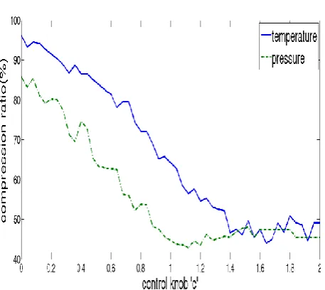
In IR-LDCA, the value of control knob c (used in equation (3)) can be altered to get the corresponding compression ratio for each parameter (temperature, pressure). In the graph shown in Fig.1 the compression ratios for various values of c have been indicated for both pressure and temperature quantities. The compression ratio depends on the value of c. The x-axis of the graph shown in Fig. 1 represents the variable values for the control knob c and the y-axis represents the compression ratio obtained. The value of the compression ratio for temperature decreases gradually from 95.4% to 45% and the pressure decreases from 85.8% to 45.4%, as the value of c changes from 0 to 2. The line graph thus obtained shows a gradual change in compression ratio as the value of c changes. This is because- as the value of c increases, the value of delta decreases and this results in lowering of the compression ratio. It is observed that, most of the times, the change in compression ratios for both temperature and pressure show similar behavior (both of them either increase or decrease), between any pair of values for c. This is due to the fact that the data samples are not mutually correlated.

.

Figure.1: Compression ratios achieved for varying values of c for temperature and pressure

Figure.2: RMS error percentage for varying values of c for temperature.

Figure.3: RMS error percentage achieved for varying values of c for temperature and pressure.

The RMS error percentage (RMS error*100) for varying value of c, for temperature and pressure, are plotted in Fig. 2. and Fig 3. respectively. In both the graphs, c is plotted on the x-axis and the y-x-axis represents the error percentage obtained. The value of the error percentage for temperature decreases gradually from 7.75% to 0.072% in Fig. 2, as value of c changes from 0 to 2. In Fig. 3, the graph shows decrease in the error percentage for pressure from 6.95% to 0.0684%. The line graph thus obtained shows a gradual change in error percentage when the value of c changes. This is because, as the value of c increases, the value of delta decreases resulting in decreased error percentage.

4.3

Comparison between IR-LDCA and

K-RLE

algorithms. In order to make a comparison between K-RLE and the proposed IR-LDCA, the value of K is considered as the standard deviation of the data sample and c corresponding to their respective highest compression ratios. Next, the RMS error as a percentage of range of the values in the data set is obtained to compare the loss generated up on the application of the two algorithms.

Figure.4. Compression ratios achieved in K-RLE and IR-LDCA for temperature and pressure.

The compression ratio obtained for K-RLE is 99.7% and 99.4% for temperature and pressure respectively. In case of IR-LDCA, it is 96.2% and 85.8% for both parameters. The compression ratios given here for IR-LDCA are corresponding to the minimum value of c.

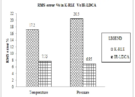
Figure.5. RMS error percentage in K-RLE and IR-LDCA for temperature and pressure.

The error percentage obtained for K-RLE is 17.2% and 20.5% for temperature and pressure respectively. In case of IR-LDCA, it is 7.75% and 6.95% for both temperature and pressure respectively. The results obtained reveal the fact that the improvement in the compression ratio in IR-LDCA against that of the K-RLE is nominal, but IR-LDCA shows a drastic reduction in RMS error percentage, when compared to that of K-RLE. Reducing the value of ‘c’ below 0 can yield greater compression ratios at the cost of higher losses which in comparison to that of K-RLE is less. Also, the fact that in the algorithm the user has the chance of controlling ‘c’ and hence, controlling the value of compression ratio and error percentage. Whereas in K-RLE the value of K is taken to be

the Standard or Allan deviation of the data set, giving it less opportunity to control the error. This proves the advantage of our IR-LDCA over the existing K-RLE algorithm making it more flexible compared to the existing algorithm.

5.

CONCLUSION

In this paper, a new lossy data compression algorithm, IR-LDCA for WSNs is proposed to achieve energy efficiency in transmission. The proposed algorithm, effectively exploits the natural correlation that exists in sensor data. The objective of the work was to exploit the commonality existing in the continuous data stream and also to eliminate redundancy. This property was exploited by inducing redundancy in the data set by converting them to their integer representation using equation (4). This lossy data compression scheme allows the user to control the compression ratio desired and the data loss during the compression facilitating higher compression ratios with minimum loss of data. Also, the algorithm performs in a more flexible and optimized manner than the existing K-RLE algorithm with respect to the RMS error (data loss). This proposed scheme reduces the volume of data for transmission at a sensor node (with minimal loss). Thus, resulting in reduced energy consumption and enhanced lifetime of the network.

6.

REFERENCES

[1] Akylidiz, I.F., Su, W., Sankarasubramanium, Y., Cayirci, E.: The survey on sensor networks,IEEE communications Magazine 40(8), 114-120(2002).

[2] Wang, F., and Liu, J.: Duty-cycle-aware broadcast in wireless sensor networks, in Proceedings of the 28th IEEE Conference on Computer Communications (INFOCOM '09), pp. 468-476, April 2009.

[3] Krishnamachari, B., Estrin, D., and Wicker, S.: Impact of Data Aggregation in Wireless Sensor Networks, International Workshop on Distributed Event-Based Systems, (DEBS’02) Vienna, Austria, July 2002.

[4] Fasolo, E., Rossi, M., Widmer, J., and Zorzi, M.: In-network aggregation techniques for wireless sensor networks: a survey, IEEE Transactions in Wireless Communications., vol. 14, no. 2, 70–87, April 2007.

[5] Sadler, C.M. and Martonosi, M.: Data compression algorithms for energy-constrained devices in delay tolerant networks, 4th International Conference on Embedded networked sensor systems (SenSys ’06), 265– 278, 2006.

[6] Kusuma, J., Doherty, L., and Ramchandran, K.: Distributed compression for sensor networks, Proceedings of the International Conference on Image Processing (ICIP’01) Vol. 1 IEEE, Thessaloniki, Greece, 82–85, 2001.

[7] Francesco, M., Vecchio, M.: A simple algorithm for data compression in wireless sensor networks. Communications Letters, IEEE, 12(6) :411–413, June 2008.

[9] Tharini, C., and Ranjan, P.V.: Design of Modified Adaptive Huffman Data Compression Algorithm for Wireless Sensor Network, Computer Science, vol. 5, no. 6, pp. 466–470, 2009.

[10] Salomon, D., Data Compression: The Complete Reference, Second edition, 2004.

[11] Schoellhammer, T., Greenstein, B., Osterweil, E., Wimbrow, M., and Estrin, D.: Lightweight temporal compression of microclimate datasets, First IEEE Workshop on Embedded networked Sensors (EmNetS-I), Tampa, Florida, USA, November 2004.

[12]Intel Berkeley Research lab,