Parallelizing Apriori on Dual Core using OpenMP

(1)

Parallelizing Apriori on Dual Core using OpenMP

Anuradha.T

ANU,Guntur

A.P.,INDIA

Satya Pasad R

ANU,Guntur

A.P.,INDIA

S.N.Tirumalarao

NEC,Guntur A.P.,INDIA

ABSTRACT

Accumulation of abundant data from different sources of the society but a little knowledge situation has lead to Knowledge Discovery from Databases or Data Mining. Data Mining techniques use the existing data and retrieve the useful knowledge from it which is not directly visible in the original data. As Data Mining algorithms deal with huge data, the primary concerns are how to store the data in the main memory at run time and how to improve the run time performance. Sequential algorithms cannot provide scalability, in terms of the data dimension, size, or runtime performance, for such large databases. Because the data sizes are increasing to a larger quantity, we must use high-performance parallel and distributed computing to get the advantage of more than one processor to handle these large quantities of data. The recent advancements in computer hardware for parallel processing is multi core or Chip Multiprocessor (CMP) systems. In this paper we present an efficient and easy technique for parallelization of apriori on dual-core using openMP wih perfect load balancing between the two cores. We present the performance evaluation of apriori for different support counts with different sized databases on dual core compared to sequential implementation

General Terms

Data Mining, Parallel Processing

Keywords

Data Mining, Parallel Processing

1. INTRODUCTION

Data Mining deals with large volumes of data to extract the previously unseen and useful knowledge (1,2).Association Rule mining (ARM) or frequent itemset mining is an important functionality of Data Mining(3). The apriori algorithm (4) is one of the best algorithms for finding frequent itemsets from a transactional database. It requires scanning the entire database more number of times. As Data Mining mainly deals with large volumes of data, the main concern should be how to improve the performance of the algorithm. One way of improving the performance of apriori is parallelizing the algorithm (5, 6). The recent advancement in computer hardware for parallel processing is Multi-Core architectures(7,8).In this paper we present the performance evaluation of parallelization of apriori for different sized databases with different support counts on a dual core system compared to its sequential implementation using an efficient and easy technique with perfect load balancing between the processors.

2. Related Work

Apriori algorithm is the first algorithm proposed for frequent itemset mining which depends on candidate generation (4, 9). Han et al. proposed FP-growth method for frequent itemset mining without candidate generation (10). Apriori and FP-growth methods use horizontal data format to represent the transactional database. Zaki proposed Eclat algorithm for

frequent itemset mining using vertical data format(11). To handle the

scalability problem of sequential algorithms, parallel and distributed algorithms are proposed(12).Rakesh Agrawal, John C.Shafer proposed the first two parallel association algorithms count distribution and data distribution (13). David W. Cheung et al. proposed a distributed association rule mining algorithm FDM, which reduces the number of messages to be passed at mining association rules (14). Mohammed J. Zaki presented a survey on parallel and distributed association rule mining (6).Zaıane et al. proposed a parallel algorithm for mining frequent patterns using FP-Growth mining (15).Wenbin Fang et al. presented two implementations of frequent itemset mining on new generation Graphics processing units (16).Shirish Tatikonda et al. discussed mining subtrees from a tree structured data by considering various memory optimizations in (17). Li Liu et al. proposed a cache-conscious FP-array (frequent pattern array) and a lock-free dataset tiling parallelization mechanism to parallelize frequent itemset mining on multi core using FP-tree based mining(18).

3. LITERATURE

3.1 Multi core

Multi core refers two or more processors. But they differ from independent parallel processors as they are integrated on the same chip circuit (7,8).A multi core processor implement message passing or shared memory inter core communication methods for multiprocessing. If the number of threads are less than or equal to the number of cores, separate core is allocated to each thread and threads run independently on multiple cores. (Figure 1) If the number of threads are more than the number of cores, the cores are shared among the threads.

Any application that can be threaded can be mapped efficiently to multi-core, but the improvement in performance gained by the use of multi core processors depends on the fraction of the program that can be parallelized.[ Amdahl's law] (19)

Figure 1: Independent threads on the cores

c o r e

1

c o r e

2

c o r e

3

c o r e

4

(2)

3.2 OpenMP

OpenMP (Open Multi Processing) is an application program interface (API) that supports multi-platform shared memory multi processing programming in C/C++ and Fortran on many architectures(20,21,22).It consists of a set of compiler directives. OpenMP uses Fork-Join Parallelism to implement multi threading.

3.3 Fork-Join Parallelism

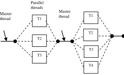
[image:2.595.94.299.292.416.2]

Initially programs begin as a single process: master thread. We can make some part of the program to work in parallel by creating child threads. Master thread executes in serial mode until the parallel region construct is encountered. Master thread creates a team of parallel child threads (fork) that simultaneously execute statements in the parallel region. The work sharing construct divides the work among all the threads. After executing the statements in the parallel region, team threads synchronize and enumerate (join) but master continues (Figure 2).

Figure 2: Fork-Join parallelism

4 .ASSOCIATION RULE MINING

The concept of Association rule mining was originated from the market basket analysis (3). It considers a transactional database D which consists of the transactional records of the customers {T1,T2,…,Tn}. Each transaction T consists of the items purchased by the customers in one visit of the super market. The items are the subset of the set of whole items I in the super market we are considering for analysis. We represent I as the set {I1, I2,…., Im}.An itemset consists of some combination of items which occur together or a single item

from I. Association rule mining X



Y, represents the

dependency relationship between two different itemsets X and Y in the database. The relationship is whenever X is occurring in any transaction, there is a probability that Y may also occur in the same transaction. This occurrence is based on two interesting measures.

1.Support= percentage of transactions in D that contain XUY 𝑠𝑢𝑝𝑝𝑜𝑟𝑡 𝑋 = 𝑃(𝑋 ∪ 𝑌)

2.Confidence=percentage of transactions in D containing X that also contain Y.

𝑐𝑜𝑛𝑓𝑖𝑑𝑒𝑛𝑐𝑒 𝑋 𝑌 = 𝑃(𝑌 𝑋 )

Finding the association rules for any given transactional database consists of two parts:

1. Finding the frequent itemsets—Frequent itemsets are the itemsets which are having a frequency more than a predefined minimum support count (min_sup).

2. Generation of Association rules— Rules generated from the subsets of a frequent itemset.

The major part of this rule mining is finding frequent itemsets. Apriori algorithm is the popular algorithm for finding the frequent itemsets.

4.1 The Apriori algorithm

It is based on the apriori property that all nonempty subsets of a frequent itemset must also be frequent (4). It is a two step process.

Step 1: The Prune Step: The entire database is scanned to find the count of each candidate in Ck. Ck represents candidate k-itemset. The count each itemset in Ck is compared with a predefined minimum support count to find whether that itemset can be placed in frequent k-itemset Lk.

Step 2: The join step: Lk is natural joined with itself to get the next candidate k+1- itemset Ck+1.

The major step here is the prune step which requires scanning the entire database for finding the count of each itemset in every candidate k-itemset. So to find all the frequent itemsets in the

database, it requires more time if the database size is more.

4.2 Parallelizing apriori on dual- core using

openmp

In parallelizing apriori on dual-core, we use the fork–join concept of OpenMP for finding frequent k- itemset.

Pseudocode for apriori on dualcore

//All the items in the database will be in candidate 1-itemset , C1.For each item in C1, the following procedure will be followed.

1. divide the database into 2 partitions. 2. select a minimum support count ,min_sup. 3. SET_ OMP_NUM_THREADS =2 4. /* start of parallel code

#pragma omp parallel #pragma omp sections {

omp section {

//partition1 find_count1(i) }

omp section {

//partition2 find_ count2(i) }

} /* implicit barrier */

//The first section calculate the count of items in partition1 and second section calculate the count of items in partition 2 . 5. sum up the counts of each partition separately

for each item[i] in C1 and if count[i]>min_sup ,place item[i] in frequent 1-itemset,L1.

6. Join L1 with itself to get C2 where the items are of the type (i,j).

7.Go to step 4 for finding count of items in C2.

8.Repeat this process until L k=



.

5. EXPERIMENTAL WORK

For our experimentation, we have used Intel Pentium Dual-Core 1.60 GHz processors with 3GB RAM. We have used Fedora 9 Linux (Kernel 2.6.25-14, Red Hat nash version 6.0.52) equipped with GNU C++ (gcc version 4.3) in our study. We have used OpenMP threads to study their performance on dual-Core processors. In our experiments randomly generated data sets are used. Random data sets are generated separately to have 1 to 10 lakh records with 10 different items,I1 to I10.Our algorithm is tested with different support counts 5%,10%,15%, 20%,30%,

T1

T2

T3

T1

T2

T3

T4

Master thread Master

thread

(3)

35% 40%,45% and 50% for each dataset. First the program is implemented sequentially and then it is implemented on dual core processors using openMP threads. Perfect load balancing will be done as each thread will take only 50% of the data. To know the time consumed by the program in different environments, we have used time command of Linux .This command gives the real time, user time and system time. These timings are noted by varying datasets and for each dataset by varying different support counts for single core and dual core implementations.

5.1 Comparison with related Work

We have parallelized apriori in our work using the concept similar to count distribution (CD) algorithm discussed in (13). In count distribution also database is partitioned and each processor is responsible for only locally stored transactions. But in count distribution algorithm a hash-tree corresponds to all the candidates is built and it is partitioned among processors but our implementation does not build any hash tree. Because of the overhead in constructing the hash tree, CD algorithm does not perform well with respect to increasing the number of candidates that is by lowering minimum support count(23) But our implementation perform well at lower minimum support counts. In Data distribution (DD) algorithm the candidate itemsets are partitioned among the processors. And both CD and DD algorithms are implemented on individual parallel processors. But our implementation is done on dual core processor. Shirish Tatikonda et al. (17) discussed parallelizing on multi core but they have worked with mining subtrees from a tree structured data and our implementation deals with frequent itemset mining. Li Liu et al.(18) proposed frequent itemset mining on multi core using FP-tree based mining and our implementation uses apriori algorithm.

5.2 Experimental Results

Our experiments gave the following observations:

1. There is a run time performance improvement by parallelizing the apriori algorithm on dual core compared to sequential implementation.

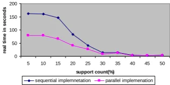
2. For any dataset with different support counts, real time consumed by the algorithm on dual core is less than that of the time consumed for sequential execution (Figure 3 to Figure 12). The benefit of dual core in real times can be observed more at lower support counts than at higher support counts that means when the frequent itemsets generated are more. (Figure 13 to Figure 22).

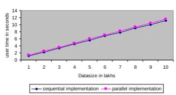
3. But we can observe only a slight reduction in the user time on dual core compared to sequential execution at lower support counts and user time on dual core is slightly more than sequential execution at higher support counts.(Figure 25 to Figure 28)

4. For any dataset , when the support count is increasing, the real time and user time consumed will be decreasing on both sequential and parallel implementations if the frequent itemsets generated are different for those support counts. (Figure 3 to Figure 12,Figure 23,Figure 24).

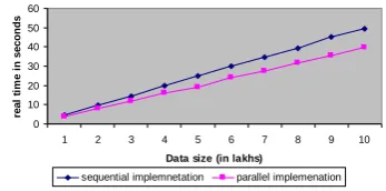
5.For any support count , when the dataset size is increasing, the real and user time consumed will be increasing on both sequential and parallel implementations.(Figire 13 to Figure 22,Figure 25 to Figure 28)

[image:3.595.341.524.123.230.2]

5.3 Real time Observations for different

support counts with fixed data sizes

[image:3.595.348.517.275.359.2]

Figure 3 : One lakh data with varying support counts

[image:3.595.348.517.406.490.2]

Figure 4: Two lakh data with varying support counts

Figure 5:Three lakh data with varying support counts

Figure 6: Four lakh data with varying support counts

Data size=1lakh records

0 10 20 30 40 50 60

5 10 15 20 25 30 35 40 45 50

support count(%)

re

a

l

ti

m

e

i

n

s

e

c

on

ds

sequential implemnetation parallel implemenation

Data size=2lakh records

0 20 40 60 80 100 120

5 10 15 20 25 30 35 40 45 50

re

a

l

ti

m

e

i

n

s

e

c

on

ds

Data size=3 lakh records

0 50 100 150 200

5 10 15 20 25 30 35 40 45 50

re

a

l

ti

m

e

i

n

s

e

c

on

ds

Data size= 4 lakh records

0 50 100 150 200 250

5 10 15 20 25 30 35 40 45 50

re

a

l

ti

m

e

i

n

s

e

c

on

ds

[image:3.595.347.517.535.622.2]

(4)

[image:4.595.92.264.75.178.2] [image:4.595.348.517.77.178.2]

Figure 7: Five lakh data with varying support counts

[image:4.595.92.264.221.323.2]

Figure 8: Six lakh data with varying support counts

[image:4.595.349.516.248.337.2]

Figure 9: Seven lakh data with varying support counts

[image:4.595.91.264.367.454.2]

Figure 10: Eight lakh data with varying support counts

Figure 12: Ten lakh data with varying support counts

[image:4.595.348.517.379.468.2]

5.4 Real time observations for different data

sizes with fixed support counts

Figure 13: Sup_count 5% with varying datasizes

Figure16: Sup_count 20% with varying datasizes

0 50 100 150 200 250

5 10 15 20 25 30 35 40 45 50

support count(%) re a l ti m e i n s e c on ds

0 50 100 150 200 250 300 350

5 10 15 20 25 30 35 40 45 50

0 50 100 150 200 250 300 350 400

5 10 15 20 25 30 35 40 45 50

0 100 200 300 400 500

5 10 15 20 25 30 35 40 45 50

0.00 100.00 200.00 300.00 400.00 500.00 600.00

5 10 15 20 25 30 35 40 45 50

0 100 200 300 400 500 600

5 10 15 20 25 30 35 40 45 50

Support count = 5%

0 100 200 300 400 500 600

1 2 3 4 5 6 7 8 9 10

Data size (in lakhs)

re a l ti m e i n s e c on ds

Support count = 10 %

0 100 200 300 400 500 600

1 2 3 4 5 6 7 8 9 10

0 100 200 300 400 500 600

1 2 3 4 5 6 7 8 9 10

0 50 100 150 200 250 300 350

1 2 3 4 5 6 7 8 9 10

[image:4.595.93.264.498.599.2] [image:4.595.348.516.511.598.2] [image:4.595.93.264.643.746.2] [image:4.595.349.516.644.729.2]

(5)

[image:5.595.91.264.75.178.2] [image:5.595.348.517.79.178.2]

[image:5.595.91.265.222.324.2]

[image:5.595.347.518.262.353.2]

[image:5.595.87.261.365.451.2]

5.6 User time Observations for different

support counts with fixed data sizes

Figure 23: One lakh data with varying supportcounts

Figure 24: Ten lakh data with varying supportcounts

5.7 User time observations for different

datasizes with fixed support counts

Figure 25: sup_count 5% with varying datasizes

0 20 40 60 80 100 120 140 160

1 2 3 4 5 6 7 8 9 10

0 10 20 30 40 50 60

1 2 3 4 5 6 7 8 9 10

0 10 20 30 40 50 60

1 2 3 4 5 6 7 8 9 10

0 2 4 6 8 10 12 14

1 2 3 4 5 6 7 8 9 10

0 2 4 6 8 10 12

1 2 3 4 5 6 7 8 9 10

Support count =50 %

0 2 4 6 8 10 12

1 2 3 4 5 6 7 8 9 10

data size=1 lakh records

0 10 20 30 40 50 60

5 10 15 20 25 30 35 40 45 50

support counts ( %)

us e r ti m e i n s e c on ds

sequential implementation parallel implementation

Data size=10 lakh records

0 100 200 300 400 500 600

5 10 15 20 25 30 35 40 45 50

support counts(%) us e r ti m e i n s e c on ds

support count 5%

0 100 200 300 400 500 600

1 2 3 4 5 6 7 8 9 10

datasize in lakhs

u s e rt im e i n s e c o n d s

[image:5.595.348.517.389.486.2] [image:5.595.90.265.481.583.2] [image:5.595.347.517.561.655.2] [image:5.595.91.264.625.726.2]

(6)

[image:6.595.91.264.75.178.2] [image:6.595.89.264.208.307.2]

7. CONCLUSIONS

Apriori algorithm is parallelized on dual core using a simple and efficient technique with perfect load balancing between the cores. The run time performance of parallelization of apriori on dual core is compared to sequential execution with different support counts for different databases. There is a clear run time performance improvement of parallelizing the algorithm on dual core in terms of real time compared to sequential implementation on single core. In our future work we study the performance of apriori on dual core by changing the number of threads.

8. REFERENCES

[1] Jiawei Han and Micheline Kamber 2006 ‖Data Mining concepts and Techniques‖, 2nd edition Morgan Kaufmann Publishers, San Francisco.

[2] Fayyad, Usama,Gregory Piatetsky-Shapiro, and Padhraic Smyth 1996 "From Data Mining to Knowledge Discovery in Databases". AI Magazine Volume 17 Number 3(1996)

[3] Agrawal R, Imielinski T, Swami A 1993 ―Mining association rules between sets of items in large databases‖ In: Proceedings of the 1993ACM-SIGMODinternational conference on management of data (SIGMOD‘93), Washington, DC, pp 207–216

[4] Agrawal R, Srikant R 1994 ―Fast algorithms for mining association rules‖ In: Proceedings of the 1994 international

conference on very large data bases (VLDB‘94), Santiago, Chile, pp 487–499

[5] R. Agrawal and J. Shafer 1996 ―Parallel mining of association rules‖ IEEE Trans. Knowl. Data Eng., vol. 8, pp. 962–969, Dec. 1996.

[6]M.J. Zaki 1997 ―parallel and distributed association mining:A survey‖IEEEConcur,vol. 7, pp. 14–25, Dec. 1997.

[7] Herb Sutter 2005 ―The Free Lunch Is Over A Fundamental Turn Toward Concurrency in Software‖ This article appeared in Dr. Dobb's Journal, 30(3), March 2005. [8] N.Karmakar 2011 ―The New Trend in processor Making

Multi-Core Architecture‖ www.scribd.com 15th may2011 [9] Jiawei Han, Hong Cheng,Dong Xin, Xifeng Yan 2007

―Frequent pattern mining: current status and future directions‖ In the Journal of Data Min Knowl Disc (2007) 15:55–86,Springer Science+Business Media, LLC 2007. [10] Han J, Pei J, Yin Y 2000 ‖ Mining frequent patterns

without candidate generation‖ In: Proceeding of the 2000 ACM-SIGMOD international conference on management of data (SIGMOD‘00),Dallas, TX, pp 1–12

[11] ZakiMJ 2000 ―Scalable algorithms for association mining‖ IEEETransKnowl Data Eng 12:372–390

[12]Park JS, Chen MS, Yu PS 1995 ―Efficient parallel mining for association rules‖ In: Proceeding of the 4th international conference on information and knowledge management, Baltimore, MD,pp 31–36

[13] Agrawal R, Shafer JC 1996 ―Parallel mining of association

rules: design, implementation, and experience‖ IEEE Trans Knowl Data Eng 8:962–969

[14] Cheung DW, Han J, Ng V, Fu A, Fu Y 1996 ―A fast

distributed algorithm for mining association rules‖ In: Proceeding of the 1996 international conference on parallel and distributed information systems, Miami Beach, FL, pp 31–44

[15] O. R Zaiane,M. El-Hajj, and P. Lu 2001 ―Fast parallel association rule mining without candidacy generation‖ in Proc. ICDM, 2001, [Online].Available: citeseer.ist.psu.edu/474 621.html, pp. 665–668.

[16] Wenbin Fang, Mian Lu, Xiangye Xiao, Bingsheng He, Qiong Luo 2009 ―Frequent itemset mining on graphics processors‖ Proceedings of the Fifth International Workshop on Data Management onNew Hardware (DaMoN 2009) June 28, 2009, Providence, Rhode-Island [17]. Shirish Tatikonda, Srinivasan Parthasarathy ―Mining

TreeStructured Data on Multicore Systems‖, VLDB ‘08, August 2430,2008, Auckland, New Zealand

[18] Li Liu2, 1, Eric Li1, Yimin Zhang1, Zhizhong Tang 2007 ‖Optimization of Frequent Itemset Mining on Multiple-Core Processor‖ VLDB ‗07, September 23-28, 2007, Vienna, Austria.

[19] Amdahl, Gene 1967 "Validity of the Single Processor Approach to Achieving Large-Scale Computing Capabilities". AFIPS Conference Proceedings (30): 483– 485.

sup count=20%

0 50 100 150 200 250 300 350

1 2 3 4 5 6 7 8 9 10

Datasize in lakhs

us

e

rt

im

e

i

n

s

e

c

on

ds

sup count =35%

0 10 20 30 40 50 60

1 2 3 4 5 6 7 8 9 10

Datasize in lakhs

u

s

e

r

ti

m

e

i

n

s

e

c

o

n

d

s

sup count =50%

0 2 4 6 8 10 12 14

1 2 3 4 5 6 7 8 9 10

Datasize in lakhs

u

s

e

r

ti

m

e

i

n

s

e

c

o

n

d

s

[image:6.595.90.264.342.436.2]

(7)

OpenMP Architecture Review Board.http://www.openmp.org/

[21] Kent Milfeld 2011 ―Introduction to Programming with OpenMP‖ September 12th 2011, TACC

[22] Ruud van der pas 2009 ―An Overview of OpenMP‖ NTU Talk January 14 2009