Forecasting methods: a comparative analysis

Munich Personal RePEc Archive

Forecasting methods: a comparative

analysis

Iqbal, Javed

Karachi University

2001

Online at

https://mpra.ub.uni-muenchen.de/23856/

Proc. Eighth Stat. Sem. 2001, K.U. ISBN-969-8397-07-8-(189-197)

FORECASTING METHODS: A COMPARATIVE ANALYSIS

Javed Iqbal

ZYXWVUTSRQPONMLKJIHGFEDCBA

D e p a r t m e n t o f S t a t i s t i c s , U n i v e r s i t y o f K a r a c h i

ABSTRACT

Forecasting is an important tool for management, planning and administration in various

fields. In this paper forecasting performance of different methods is considered using time series data of

Pakistan's export to United Sates and money supply. It is found that, like other studies of this nature, no

single forecasting method provides better forecast for both the series. The techniques considered are

ARIMA, Regression Analysis, Vector Autoregression (VAR), Error Correction Model (ECM) and

ARCH/GARCH models.

1.

INTRODUCTION

Forecasting is a probabilistic estimate or a description of a future value or condition, which

includes a mean, range and probability estimate of that range. There is a considerable literature on

forecasting in business and economics. Some are aimed at forecasting a particular variable of interest

e.g. stock prices, money demand, exchange rates etc. for example Chan and Lee (1997), Kumar (1992),

Bhawnani and Kadiyala (1997), Bleaney (1998). Others focus on a comparison of different models or

techniques of forecasting, LeSage (1990), Stock and Watson (1996), Fair (1973). This study is of later

style. A distinguishing feature of this study is the presentation of forecast confidence intervals besides

mean forecasting. The models considered are univariate as well as multivariate. To broaden the scope,

the time series considered are quarterly as well as annual. The annual data (1972-1999) for forecasting

State Bank's money supply (M2) is used. Forecasting this variable is important for potential investors

since money supply affects interest rate and consequently investment. It also has an impact on prices.

An estimate of this variable is important for Central Bank itself so that to achieve its target of

stabilizing the economy, some alteration in historical pattern of money supply could be made. Secondly

quarterly data (1988:1 -1999:4) for forecasting Pakistan's export to U.S., a major trading partner of

Pakistan, is considered. The export function involves a variable of economic activity of trading partner

(U.S. in this case for which the data are available) instead of the home country. This variable is chosen

keeping in view the availability of quarterly data. Since macroeconomic models usually involve a

variable of real economic activity such as GDP, or its component. Unfortunately quarterly data for

Pakistan on these real variables are not available. The data are collected from various issues of State

Bank's monthly bulletin and IMP's International Financial Statistics. The results of almost all studies of

this nature indicates that no single model camouflage as the best for out-sample forecasting of different

series. This study also provides such an evidence.

Export Function:

E=f(YA,RP, V) (1.1)

Where E: Pakistan's export to U.S (millions of U.S $), YA: United State's GDP (Billions of U.S.$

consumer price index. V: Exchange rate volatility computed as in Ariz and Shwiff (1998) as an eight

quarter moving standard deviation i.e.

ZYXWVUTSRQPONMLKJIHGFEDCBA

( 1 . 2 )

Where RI is the exchange rate (Rs per U.S.$) and RI is its forecasted value (ARIMA model has been

used to forecast it)

Expected signs of the coefficients of the explanatory variables are as follows:

ZYXWVUTSRQPONMLKJIHGFEDCBA

d E > 0 d E < 0 d Y A 'd R P ,

d E < 0

av

'

Money Demand function:

M = f(Y, I) (1.3)

M: Money balances (M2) (millions of 1981 RS), Y: GDP (millions of RS) at 1981 prices, I: Nominal

interest rate on 2-3 years deposits. Expected signs are as follows:

d M > 0 d M < 0 d Y , d l

FOllowing this introduction, section 2 describes forecasting models considered in this study.

Out-sample forecasting is compared in section 3 and section 5 provides conclusion and comments.

2. FORECASTING MODELS

a) ARIMA One of the most popular univariate forecasting model proposed by Box and Jenkins

(1970). For a stationary time series

Yh

an ARMA(p,q) model is expressed as

( 2 . 1 )

where e , is a white noise disturbance term normally and independently distributed with mean

0

and

variance C J2 •

This model can be expressed as weighted sum of disturbances e , as

(2.2)

Where IJIweights are functions of the modal parameters <p's and f)' s .

An h-step ahead forecast error variance FEV (h) for y is given by

A 95% forecast confidence interval for h-step ahead forecast is given by

Yr+h

ZYXWVUTSRQPONMLKJIHGFEDCBA

±

1.96~

FEV(h) (2.4)

b) Regression Analysis A general linear regression model is given by:

(2.5)

Which in matrix form is given by

Y =

ZYXWVUTSRQPONMLKJIHGFEDCBA

x /3 +e .Where the dimensions of y is n

x

l , that of x is n

x

k, of

13

is k

x

1 and

e

is an n

x

1 vector of white noise errors with covariance matrix

L

= a2I

Let Xo

=

[ 1 X02X03... xod' be the vector of values for which forecast is required, then Y O ! x O

=

x ~ /3 .

Forecast error variance F E V (h) is given by

(2.6)

c) ARCWGARCH model The autoregressive conditional hetroskedasticity (ARCH) model

introduced by Engle

(1982)

is extensively used to model financial time series which are believed to

have varying conditional variance or volatility e.g. stock prices, interest rate, inflation etc. In this

method, mean and variance are modeled simultaneously. An ARCH model of order q is expressed

as

Y r = x r Y + £ r Where e, -N(O,a/) and

(2.7)

ARCH model were generalized by BoIIerslev (1986) as GARCH (Generalized ARCH), in

which the conditional variance depends on past value of itself. The conditional variance in a GARCH

(p,q) model is expressed as

(2.8)

The most widely used of these models is GARCH (1,1) for which the conditional variance is given by

(2.9)

The forecast error variance in GARCH models is given by ar2

d) Vector Autoregression (V AR) V AR introduced by Sim (1980), is used to model interrelated time

series simultaneously. This model, unlike structural multi-equation econometric models, relies little on

economic theory. Each variable in the model is expressed as function of the lagged values of all the

endogenous variables in the system. A V AR of order p is given by

Y ,

rqponmlkjihgfedcbaZYXWVUTSRQPONMLKJIHGFEDCBA

==A l Y ,_ I

ZYXWVUTSRQPONMLKJIHGFEDCBA

+ A 2 Y ,-2 + + A p Y ,_ p +

c,

(2.10)

Where e , - N (O,Q) is a vector of white noise errors with covariance matrix Q. The errors are assumed

to be serially independent in each equation but they may be contemporaneously correlated across

equations. Ai'S (i =1 ,2, ... ,p) are the matrices of the coefficients to be estimated. Yt is a vector

endogenous variables. For our export model Yt

=

[E, Y A, RP, V)'. A V AR model, unlike structural

multi equation modes, does not require the knowledge of explanatory variable for forecast period.

An h-step ahead forecast of Yt is

Y t+ h == A I Y t+ h - 1 + A 2 Y t+ h -2 + + A p Y '+ h _ p (2.11)

Where Y t+ h - I , , Y t+ 1 are forecasted using similar scheme. For a YAR (1), we have

Y t+ h == A Y ,+ h - 1 and forecast error variance (as given in Clement and Hendry (1993» is

h - i

FEV(h) == L A jQ ( Aj)'. With normality assumption, we can derive simple expression for the forecast

j=O

intervals for individual time series by considering the diagonal elements of FEV (h) matrix.

e) Error Correction Model (RCM) It is widespread in modem econometric literatu~e that a

regression involving non-stationary time series variables may be spurious or misspecified unless the

variables are Co-integrated. The time series XII and x_2, each integrated of order 1, are said to be

co-integrated if any linear combination.if these e.g.

Cz,

==a lx l, + a_{2x 2 ,)} is stationary. The concept of

co-integration in statistics is equivalent to stable long run relationship in economics. The short run

disequilibrium can be modeled as an error correction model.

To get the idea lets consider a time series regression

Y , = = a + f3 'x ,

+c,

(2.12)

Where Y , is the dependent variable and x , is a vector of independent variables. If Y , and x , are in

equilibrium, then the error Y , - a - f3 'x , will equal zero. However in disequilibrium it will be non-zero.

This quantity measures the extent of di equilibrium between Y ,and x , and hence is called

disequilibrium error. In disequilibrium Y ,can be assumed to be related with x , and the lagged values

of Y ,and x " one typical form of which is

(2.13)

Subtracting Y ,_ I from each side of eq (2.13) above and reparametezing we get

(2.14)

Where the parameter J..I. depends on parameters in eq (2). The term in bracket is called the error

correction term, which incorporates past period's disequilibrium. Eq (2.14) is an example of error

· long run equilibrium relationship between non-stationary variables is estimated. In our present case this

would be the regression E

=

f (Y A, RP, V) for export function, In the second step ECM model eq

(2.14) is estimated using residuals lagged one period from the long run regression. Forecasting of y can then be performed using the ECM model and the forecast error variance is given as eq (2.6).

3-

FORECAST COMPARISON

The comparison of forecasting models is based on Root Mean Square Error (RMS)

(3.1)

and Theil's Inequality Coefficient

ZYXWVUTSRQPONMLKJIHGFEDCBA

( U )

(3.2)

The former depends on the unit of measurement of the variable to be forecasted and later is

unit free lying between 0 and 1 with the forecast getting better as the

U

is closer to

O.

These measures are widely used for out-sample forecasting e.g. in Chan and Lee (1997) and

[image:6.616.13.589.20.730.2]

Kumar (1992) among others.

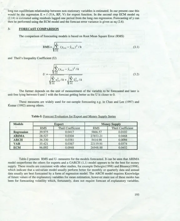
Table-I:

Forecast Evaluation for Export and Money Supply Series

Models

Export

Mone

RMS Theil Coeffici ent RMS

Regression

39.975 0.0417 5866.57

A'RIMA

28.527 0.0304 27853.21

ARCH

36.330 0.0381 5414.98

VAR

35.421 0.0367 22119.91

ECM

96.092 0.0948 26948.88

Table-I presents RMS and U- measures for the models forecasted. It can be seen that ARIMA

model outperforms the others for exports and a GARCH (1,1) model appears to be the best for money

supply. These results are consistent with other studies, for example Delurgio(1998) and Bleaney(1998), which indicate that a univariate model usually perform better for monthly or quarterly data and annual

data usually are best forecasted by a form of regression model. The ARCH model requires Knowledge

of future values of the explanatory variables for mean estimation, however main use of these modes has been for forecasting volatility which, fortunately, does not require forecast of ,explanatory variables.

[image:7.613.7.585.14.722.2]

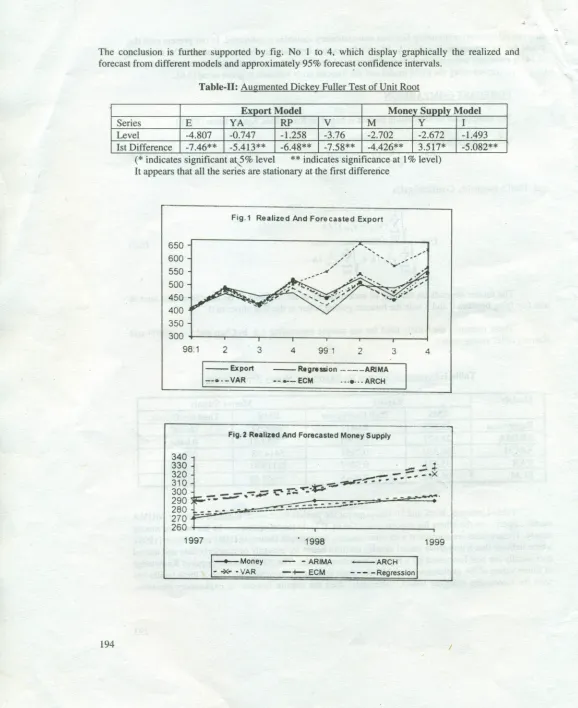
The conclusion is further supported by fig. No I to 4, which display graphically the realized and forecast from different models and approximately 95% forecas! confidence intervals.

Table-II: Augmented Dickey Fuller Test of Unit Root

Export Model Monev Sunnlv Model

Series E YA RP

ZYXWVUTSRQPONMLKJIHGFEDCBA

V M Y I

Level -4.807 -0.747 -1.258 -3.76 -2.702 -2.672 -1.493

1st Difference -7.46** -5.413** -6.48** -7.58** -4.426** 3.517* -5.082**

(* indicates significant at.2% level ** indicates significance at 1% level) It appears that all the series are stationary at the first differerice

F i g . 1 R e a l i z e d A n d F o r e c a s t e d E x p o r t

650 600 550 500 450 400 350

300

+---~----,----.----.-__~

~~~

98:1

, ,

2 3 4 991

2

3

- - E x p o r t - - • • - V A R

- - R e g r e s s i o n . • • . - - A R I M A - - • . •- E C M .·-e·· -A R C H

F i g . 2 R e a l i z e d A n d F o r e c a s t e d M o n e y S u p p l y

340

330 ~ ..:.

.+

320 _ - ~~ _oX

310 _

ZYXWVUTSRQPONMLKJIHGFEDCBA

- - .r : ~ .- ....

300

~F-- -:-;:::-

.•

- = ' ; ; ~ ; : : .- - : - ~ • • . • . . - _ .

290'-

.~----280

=-.= __

. - -~-

----270

..-260

+---.---,

1997 . 1998 1999

I

_ M o n e y- - x - · V A R

- - A R I M A

- + - E C M

- A R C H I - - - - R e g r e s s i o n I

F i g , 3 : 9 5

rqponmlkjihgfedcbaZYXWVUTSRQPONMLKJIHGFEDCBA

%F o r e c a s t I n t e r v a l s F r o m D i f f e r e n t M o d e l s O f E x p o r t

Regression ARIMA

800 800

700 700

600 600

500 500

400 400

300 300

200 200

tOO tOO

0 0

98t 99't 9 8 : 1 2 3 4 9 9 : 1 2 3 4

VAR ECM

800 600

700 700

600 600

500 500

400 400

300 300

200 200

tOO tOO

0

0

98't 99't ~3:1 2 3 4 9 9 : 1 2 3 4

ARCH

800

700

600 500 400 300 200 tOO

0

98t 991

Regression

ZYXWVUTSRQPONMLKJIHGFEDCBA

F i g . 4 : 9 5 % F o r e c a s t I n t e r v a l ! ' F r o m D i f f e r e n t M o d e l s O f M o n e y S u p p l y

rqponmlkjihgfedcbaZYXWVUTSRQPONMLKJIHGFEDCBA

·350 340 330 320

~~

---~-r---=======::

~t:t=====::=====:;

270 260

~₁₉₉₇

~---ARIMA

JSO 340 330

. - A 320

310

-

300 290

-

280 270 260 7,50

1999 1997 1996 9

1998 ARCH JSO ~ ~ 320 ~ ~==:=:=:==========:~:::=============~=-=-===-===::--1997 1998 ECM 350 . J40 330 320 310 300 290 280 170 260 z s o

1997 1998 1999

196 199!l VAR JSO ~ ~ 3JO 320

il

270 260 ~ .

4.

CONCLUSIONS

A comparison of forecasting performance of different time series econometric models is

considered using data from Pakistan's .macroeconomy. Like previous studies no single model appeared

the best for both the variables forecasted. The message revealed by the study is that to forecast a

particular variable one should not rely on a single forecasting method rather performance of different

competing models should be checked, then forecast should be performed from the best models from the

comparison.

REFERENCESZYXWVUTSRQPONMLKJIHGFEDCBA

I .

Ariz, A.C. and Shwiff, S.S. (1998). Does exchange rate volatility affects import flows in G-7

countries, evidece from Co-integration model.

ZYXWVUTSRQPONMLKJIHGFEDCBA

A p p l i e d E c o n o m i c s ,

30, 1269-1276

2.

Bhawnani, V. and Kadiyala K.R(1997).

-Forecasting foreign exchange rates indeveloping

economies.

A p p l i e d E c o n o m i c s ,

29, 51-62

3.

Bleaney,M.F. (1998). Exchange rate forecasts at the long horizon:Are error correction models

superior?

C a n a d i a n J o u n a l o f E c o n o m i c s ,

31(4), 853-864

4.

Bollersev, T. (1986).

Generalized Autoregressive Conditional Hetroskedasticity.

J o u r n a l o f

E c o n o m e t r i c s ,

31, 307-327

5.

Box, G.E.P. and Jenkins C.M. (1970). Time Series Analysis, forecasting and Control. Holden

day, San Francisco.

6.

Chan, H.L. and Lee, S.K. (1997). Modelling and forecasting the demand for coal inchina.

E n e r g y

E c o n o m i c s ,

19,271-287

7.

Clements, M.P. and Hendry, D.F. (1993). On the limitation of Comparing Mean Square

forecasting error.

J o u r n a l o f F o r e c a s t i n g ,

12,617-637

8.

Delurgio, S.A. (1998). Forecasting Principles and Application. IrvinIMcGraw Hill, Singapore.

9.

Enble, RF. and Granger, C.W.G. (1987). Co-integration and Error Correction: Represenration,

Estimation, and Testing.

E c o n o m e t r i c a ,

55,251-276

10.

Engle, RF. (1982). Autoregressive conditional Hetroskedasticity with estimation of variance of

U.K. Inflation.

E c o n o m e t r i c a ,

50,987-1008

11.

Engle, RF. and Yoo, B.S. (1987). Forecasting and testing in Co-inegrating system,

J o u r n a l o f

E c o n o m t r i c s ,

35, 143-159

12.

Fair, R. (1973). A comparison of alternative estimation of macro models.

I n t e r n a t i o n a l E c o n o m i c

R e v i e w ,

14,(2),261-273

13.

Gujrati, D.N. (1995).

B a s i c E c o n o m e t r i c s .

Mc-Graw Hill

14.

Johansen, S. (1988). Statistical Analysis of Co-inegration Vectors.

J o u r n a l o f E c o n o m i c

D y n a m i c s a n d C o n t r o l ,

12,231-254

15.

Kumar, M.D. (1992). The forecasting Accuracy of Crude Oil Futures prices.

I M F S t a f f P a p p r e s ,

39(2), 432-461

16.

LeSage, J.P. (1990). A comparison of the forecasting ability of ECM and VAR models.

R e v i e w

o f E c o n o m i c s a n d S t a t i s t i c s .

72(4), 664-671

17.

Sim, C.A. (1980). Macroeconomics and reality.

E c o n o m e t r i c a ,

48, 1-48

18.

Stock, J.H. and Watson, M.W. (1996). Evidence on Structural Instability in Macroeconomic

relations.

J o u r a n a l o f A m e r i c a n S t a t i s t i c a l a s s o c i a t i a n ,

14(1), 11-30