Parallel Computing for Accelerated Texture
Classification with Local Binary Pattern Descriptors
using OpenCL
CYN Dwith
Department of Electronic and Communication Engineering
NIT-Warangal, Warangal, Andhra Pradesh, India
Rathna.G.N,
PhD.Department of Electrical Engineering Indian Institute of Science
Bangalore, India
ABSTRACT
In this paper, a novel parallelized implementation of rotation invariant texture classification using Heterogeneous Computing Platforms like CPU and Graphics Processing Unit (GPU) is proposed. A complete modeling of the LBP operator as well as its improvised versions of Complete Local Binary Patterns (CLBP) and Multi-scale Local Binary Patterns (MLBP) has been developed on a CPU and GPU based Heterogeneous computing platforms using OpenCL. The tests using these feature descriptors of Local Binary Pattern (LBP) algorithms and their parallelized implementation using OpenCL were also performed. Significant Improvement in computation speed is achieved over traditional CPU-based algorithms. To test the accuracy of the GPU implemented algorithms a set of textures were classified using selected LBP, CLBP and MLBP descriptors. Classification was performed by applying these descriptors to several unique texture classes at various spatial resolutions and rotations. The primary focus of this paper is to provide an overview of these algorithms, demonstrate observed performance gains and to verify the validity of using these descriptors for texture analysis on a CPU and GPU based Heterogeneous Platform.
General Terms
Heterogeneous Computing, Texture Classification, Graphics Processing Unit, Parallel Programming
Keywords
Graphic Processing Unit, Local Binary Patterns, Texture Classification, Heterogeneous computing and OpenCL
1.
INTRODUCTION
In this paper we shall elaborate on how texture classification algorithms, the Local Binary Pattern operator, can be parallelized and processed by using Heterogeneous computing platforms (CPU and modern graphics hardware) using OpenCL Programming Model in image processing. Texture analysis plays a vital role in the development of many computer vision and image processing solutions. The potential applications of the texture analysis include such as biomedical image analysis, satellite surveillance systems, face recognition, inspection of industrial surfaces and object recognition. Many texture classification methods have been proposed, which assume that the samples to be classified are of similar scale, orientation and grayscale. These methods emphasize on the statistical analysis of the texture images i.e.
16
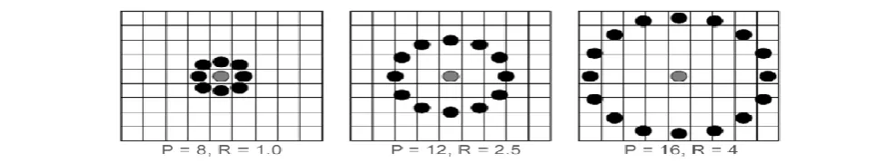
[image:2.595.318.543.97.227.2]Fig 1: Generation of Binary LBP code from the Sampled (P,R) window
Fig 2: Circular Sampling of neighbor pixels Points P at a radius R i.e. (P, R)
2.
OVERVIEW OF ALGORITHMS
2.1 LOCAL BINARY PATTERNS
Local Binary Pattern (LBP) is a very powerful tool to describe the textures and shape of a digital image. It is a simple and efficient tool to contain the texture detail, by eliminating variation in the illumination, rotation and grayscale variance. In the basic LBP operator, the neighborhood pixels of the given 3x3 window, threshold is applied with respect to the centre pixel value. The LBP operators consider only the signs of the magnitude difference, which are relatively unaffected by the variation in illumination changes, gray scale variation and other kind of noises. These signs of differences are used to generate binary code, which is converted to its equivalent decimal form to give the labels of the corresponding center pixel.
The basic LBP code is generated by comparing with its neighboring pixel values.
1
1, 0
( , ) ( , ) 0, 0
0
(
)2 , ( ) {
P
p x
P R p i j c x
p
LBP
s I
I
s x
Where
I
p i j( , ) is the pixel intensity in image at the pth sample point, where P is the total number of the sample point at a radius of R denoted by (P, R). The P circularly and evenly spaced sampling points of the window are used to calculate the difference between the centre pixel and its surrounding pixel values. It characterizes the local pattern of the image as the absolute value of the pixel are not considered and the centre pixel values are removed which make the pattern robust to any changes in the illumination conditions. These features are more effective in pattern matching then the original image patterns as they are sensitive to the noise and illumination conditions. The generalized representation of the sampling point is taken along a circle with radius R around the centre pixel as shown in Fig2. The sampling points are selected using the interpolation, if (xc,yc) are the co-ordinates of the centre pixel and the sampling points (xp,yp) are given bycos(2
/ )
p c
x
x
R
p P
sin(2
/ )
p c
y
y
R
p P
The generated local binary patterns are used to evaluate the histogram of the local region, which are cascaded to form the feature vector of the image.
( , ) 1 1
( , )
(
, ),
[0, (
1) 3]
I J
s P R
i j
H p k
f LBP
p p
P P
Where k is an integer to represent the number of sub Histograms k=[1,2,….K], K is the total number of histograms ,and f(x,y) is given by
f x y
( , ) {
1,0,x yotherwise . The generated pattern LBP pattern are further classified into Uniform and Non uniform patterns based on the number of the transition in the local binary pattern generated. In case of Uniform patterns the numbers of transitions is restricted to less than 2 i.e. (U
2), where U is the number of transitions within the circular representation of the binary pattern.( , ) 1 1
( )
( (
, ),
[0, (
1) 3]
height width
s P R
i j
H
p
U f LBP
p p
P P
Where
U x p
( , ) {
P Pp x p,( 1) 2,x pThe Uniform LBP pattern is defined as the Limited transition or discontinuities binary representation reduces the length of the histogram bin form the 2P to P (P-1) + 3 distinct output bin values. Similar to Uniform Patterns, the mapping from LBP(P,R) to rotation invariant LBP i.e.
LBP
( , )riuP R2 , which has P+2 distinct output values, given by1
( , ) 0
(
)
(
) 2
2
( , )
1
Pp c P R p
s I
I
ifU LBP
riu
P R
P
otherwise
LBP
Fig 3: Multi-scale Local Binary Pattern representation
LBP patterns are concatenated into a single feature vector to represent the LBP feature of the texture image.
2.2 Complete Local Binary Pattern (CLBP)
CLBP is an improvised version of the basic LBP operator. The LBP operator successfully eliminates the illumination and brightness variations but in turn losses some data in the image. It can be significantly improvised by the including the data pertaining to the centre pixel value and the local binary patterns can be represented at a global scale by comparing with the average gray scale pixel value.
In CLBP the locally generated patterns is quantized to binary levels after applying a global thresholding, the obtained bit map is called the LBP Center (LBPC) as it contains the data of the centre pixel values. Similarly LBP-Mean is generated by thresholding the neighboring pixel values with respect to the Mean gray scale level of the image, which are then represented as binary codes by quantizing them into two quantization levels. Where LBPS is the basic implementation of the LBP discussed earlier. Hence, in case of CLBP the basic LBP is complemented with addition data corresponding to the centre pixel and mean gray scale level, which aids in the classification and improves the efficiency of the system. The above mentioned CLBP involves the evaluation of three LBP codes maps LBPS, LBPM and LBPC. As implementation of the LBP pattern generation involves direct access to the each of the image pixels, as the size of the image increases the time complexity of the algorithm is supposed to increase linearly in case of traditional sequential approach. As CLBP involves an enormous amount of computational time to access the image pixel, in order to overcome the computational inefficiency we propose a parallelized algorithms which speeds up the CLBP feature generation to implement CLBP in real time application like face recognition systems, mobile applications, security surveillance and outdoor robotics.
In case of generation of the LBPM the values of the LBPM are given by
1
1,
( , ) 0,
0
(
,
)2 , ( , )
{
P
p x c
P R p x c
p
LBPM
s I
M
s x c
( , ) 1 1
( )
(
, ),
[0, (
1) 3]
height width
m P R
i j
H
p
f LBP
p p
P P
Where M is the mean pixel value of the image used as a threshold, and Ip is the gray scale intensity at the sampled pixel value.
In case of LBPC, the at each pixel value the thresholding is done with respect to the Mean pixel value of the whole image which is used to generate the image. The generated bit pattern is further encoded to reduce its size to 256
1, ( , )
( ,
), ( , ) {
0,x c
P R p x c
LBPC
t I M t x c
The histogram for LBPC is given by
( , )
( , ) 1, ( , ) 0 ( , ) ( , ), 0 1 1
( )
(
),
{
i j
I J
C i j I i j
c i j C i j I
i j
H k
C I
C
'
0
( )
K
c c
k
H
H k
Meanwhile, LBP technique has been able to represent the local patterns of an image very effectively. Additional discriminative information can be provided to include the centre pixel value, as well the magnitude component of the local difference within a window relative to the average gray scale value. Through CLBP we try to explore all the three types of data, for a better and efficient way of representing image features. Initially the image is represented by the gray scale values of its central pixel (LBPC), the local difference is further decomposed into the LBPS and LBPM components, finally a CLBP images, then the local histogram are generated of the each layers of the image RGB to generate the CLBP feature vector by concatenating the LBPS, LBPM and LBPC feature vectors which can be used for texture classification. These features are used for classification by using the nearest neighbor classifier with distance measurement.
2.3 Multi-Scale Local Binary Pattern
18
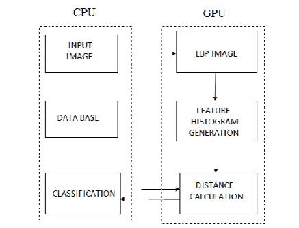
Fig 4: Implementation of LBP based LBP Operator on Heterogeneous Platform
addition, operators with different parameters can be combined to obtain a multi-scale description of texture. In Fig3, three neighborhoods with a varying number of samples (P) and different neighborhood radii (R) are shown. The corresponding LBP operators are denoted by LBPP, R. Samples that do not exactly fall on pixels are obtained with bilinear interpolation. The value of the center pixel (gray) is used as a threshold in producing a P-bit binary code that describes the local pattern in the texture. These are future classified as Uniform local patterns and rotation invariant uniform patterns. These codes have been shown to dominate the LBP distribution. The resulting operators are denoted by
2 ( , )
riu P R
LBP
. Ojala [10] reported in their experiment, that uniform patterns account for 90.6% of all patterns when using (8,1) neighborhood and 85.2% when using (8,2) neighborhood and 70% for (16,2) neighborhood. In order to reduce the feature vector length we take into consideration only the uniform patterns in the image which constitutes above 85-90% of the image data in case of (8,1) and (8,2) neighborhoods. In case of (8,1) neighborhood, the Uniform patterns effectively reduce the bin size from 256 to 59, which in turn reduces the feature vector length. This effectively reduces the length of feature vector, but still retaining almost 90% of the image data. These generated feature vectors are used to match the image from the database of image features. In [16], a multi-scale LBP was constructed by extracting a number of LBP codes for each pixel with different P and R values. The marginal distributions of these codes were used as a texture descriptor. This approach has some shortcomings, as detailed in the following. From a signal processing point of view, the sparse sampling exploited by LBP operators with large neighborhood radii may not result in an adequate representation of the two-dimensional image signal. Aliasing effects are an obvious problem. So might be noise sensitivity as sampling is made at single pixel positions, without low-pass filtering. One might argue that collecting information from a larger area would thus make the operator more robust. From the statistical point of view, even sparse sampling is however acceptable provided that the number of samples is large enough. Hence, to avoid the problem of aliasing the sampling is restricted to a radius of 3 units with 8 sampling points. To improve the performance of the algorithm and eliminate the possible aliasing effect an exponentially growing multi-resolution LBP combined with Gaussian filtering is implemented in case MLBP. These MLBP bins are further processed to generate spatial histogram, which are concatenated to form the required feature descriptor for texture classification.2.4 Metrics for Classification
We have various metrics for quantizing the difference between two feature vectors like histogram intersection, log-likelihood ratio and chi square statistics. The Chi-square statistics outperform the histogram intersection and log-likelihood statistics in terms of accuracy of detection [17].
The chi-square distance, used to measure the dissimilarity between two LBP images S and M is given by
2
1
( ,
)
(
) / (
)
L
i
D S M
Sx
Mx
Sx
Mx
Where L is the length of the feature vector of the image and Sx and Mx are respectively the values of the sample and model images at the xth bin. The Nearest-Neighborhood classifier is implemented with chi-square distance because it is equivalent to the optimal Bayesian classification [18].
3.
IMPLEMENTATION
In this section we describe the overview of the variants of LBP implementation using OpenCL model. The LBP value of a pixel is evaluated, by sampling a selected number of pixels over a circle at a distance R around the every pixel of the image. In parallelized approach, each Kernel of the OpenCL computation involves sampling P points by using circular neighborhood from selected centre pixel. The GPU based parallelized implementation involves designing a computational Kernel for evaluating the LBP values of the input Image. The Kernel takes gray scale or colored input image, the labeled pixels are updated to generate the LBP image. The parallelized algorithm is implemented as a sequence of GPU kernels using OpenCL programming language. The kernel program takes an input image and transforms it into an output image.
3.1
OpenCL Programming Model
Fig 5: Memory Model of GPU
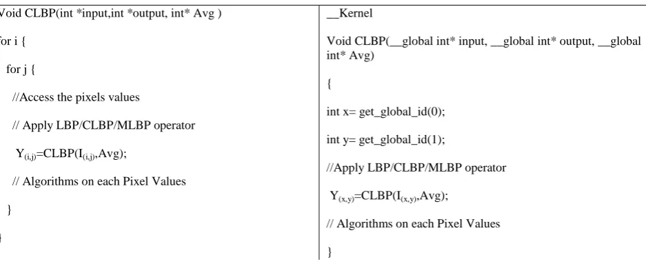
Table I:a) Pseudo-Code for CPU LBP Implementation b) Parallelized GPU Kernel
Void CLBP(int *input,int *output, int* Avg ) for i {
for j {
//Access the pixels values
// Apply LBP/CLBP/MLBP operator Y(i,j)=CLBP(I(i,j),Avg);
// Algorithms on each Pixel Values }
}
__Kernel
Void CLBP(__global int* input, __global int* output, __global int* Avg)
{
int x= get_global_id(0); int y= get_global_id(1);
//Apply LBP/CLBP/MLBP operator Y(x,y)=CLBP(I(x,y),Avg);
// Algorithms on each Pixel Values }
more effectively on SPMD platforms like GPUs. In this regard various image and video processing algorithms involve the regular access of the image pixels or frames and applying similar operation on every instance of the input, parallelizing such algorithms can boost the performance of the system by many times. The challenge related to proposed algorithm is to achieve task parallelism through a hierarchy of memory through effective utilization of memory storage area, memory bandwidth and the access and update of the data.
OpenCL is a promising language for portable GPU programming, which enables targeting heterogeneous parallel processing devices. In this section, we present a brief understanding of the names, labels and concepts, which are essential for basic understanding of the algorithm. The computational ‘kernels’ is the most important concept; it represents a function that gets executed on GPU. A ‘work item’ is used to apply the compute kernel on the input data. A group of work items is called a ‘work group’. Each work item is assigned its own location through localized and globalised work group. The local memory will be shared through local references to a work group. An extensive study of these concepts is covered in the OpenCL specifications [19]. The programming model of OpenCL broadly contains: (i) Platform Model (ii) Memory Model (iii) Execution Model.
3.1.1
Platform Model
A host (CPU) is connected to one or more OpenCL devices. OpenCL device is a collection of one or more computational unit, each computational unit is composed of multiple processing elements. Each processing elements is used to execute an SIMD (GPU) or SPMD operations.
3.1.2
Memory Model
In case of OpenCL the memory hierarchy is divided into four categories as shown in Fig5, (i) Private memory: this memory is exclusive to the work items (ii) Local Memory: this is a fast memory shared between the host processors (iii) Global Memory: this constitutes the main memory of the GPU (iv) Constant Memory: it is a part of the global memory, which is marked read only.
3.1.3
Execution Model
Data parallelism is achieved in the OpenCL through multiple work-item execution on the input image. We can define an N-dimensional computation domain (N = 1, 2 or 3). Each independent element of execution in N-D domain is called a work-item. The N-D domain defines the total number of work-items that execute in parallel i.e. processing a 512 x 512 image.
[image:5.595.69.538.574.775.2]20
Fig 8: Sample Images of Texture Classes used for Experiment
[image:6.595.57.270.577.742.2]
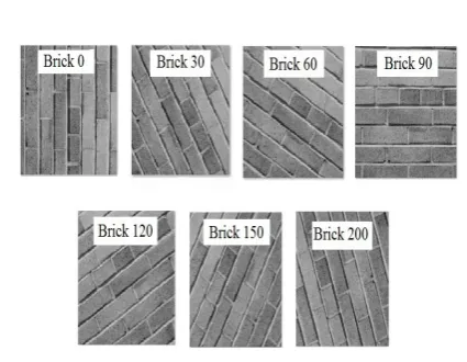
Fig 7: Sample Images of Texture Class “brick” at Different Angles of Rotation
Fig 6: Parallelized Framework for generation of CLBP using the different access layers of the image
process RGBA images, where each image pixel is 4 byte data represented by uchar4. Similarly the extended version of the vectors floatN, ucharN can also be used where N is the number of elements in the vector. We utilize the capability of the processing vector data types, four floating point represented by ‘floatn’; where ‘n’ is the number of channels accessed in parallel which can be used for RGBA image format. In case of CLBP, we use these channels to compute LBPS, LBPM and LBPC within each layer of the output image as shown in Fig6. Similarly in case of MLBP, within each layer of the image we evaluate the Multi-scale LBP using (8,1),(8,2) and (8,3) sampling.
4.
RESULTS AND ANALYSIS
The performance of the proposed algorithm was tested on AMD 6500 GPU.The feature description methods for texture classification have been evaluated against Brodatz album [20], standard benchmark texture image database. The experimental dataset included images with resolution of 256×256, 8 bits/pixel. The images are from 5 different texture classes, namely bark, brick, grass, leather and straw have been considered. The source images were rotated to obtain 7 different rotation angles of 0°, 30°, 60°, 90°, 120°, 150°, and
200°. The dataset included 10 images for each rotation angle of a texture class.
In this analysis, two images have been used to generate the texture features in each class required for the classification using Nearest-Neighbor classification and the remaining images were used as the testing sets. Therefore, both the training and the testing dataset included texture images of different illumination variations and rotation angles. The classification efficiency of the algorithms have been studied extensively in the literature [15-16, 21], hence our primary emphasis is on the execution time and performance of the algorithm on the Heterogeneous platform.
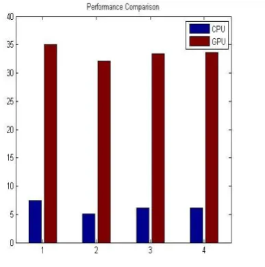
[image:6.595.319.543.578.744.2]Fig 10: Relative Improvement in the Computational Time of Different LBP operators Table II. Comparison of CPU vs OpenCL Performance in Texture Classification using Different LBP Operator
Feature Descriptor CPU ( Core 2 duo) OpenCL Model ( AMD 6500 GPU)
Classification Rate (%)
Feature Ext. Time(ms)
Classification Rate (%)
Feature Ext. Time (ms)
LBP 72.2 134.6 73.5 28.5
CLBP 76.5 197.4 75.5 31.2
MLBP ((8,1)+(8,2)) 72.45 162.6 73.45 29.9
MLBP((8,1)+(8,2)+(8,3)) 78.9 162.4 77.6 29.7
Fig 9: Computational Efficiency of CPU vs OpenCL Model (GPU)
Further, the analysis of the improvement in the computational time using GPU is tabulated in Table II, and a study of relative performance increase is depicted in the Fig9 and Fig10. Shows, that the variation of the computational time is of different LBP operators in the GPU based implementation.
5.
CONCLUSION
In this paper, we presented a reformulation of the Local Binary Pattern Operators for Texture Analysis. GPU implementation with its parallel computing paradigm outperforms the other approaches. GPUs have addressed the problem of performing image operations serially by allocating mathematical operations to multiple threads, in parallel. This enables texture analysis becomes possible even for systems with limited resources, such as mobile outdoor robots. Combined with a relatively low cost, the modern GPU is a powerful piece of computer processing hardware for its price with a wide range of applications face recognition, surveillance systems, mobile applications, texture analysis,
medical imaging, robotics and many other industrial applications.
6.
ACKNOWLEDGMENTS
This work was partially supported by AMD Development Team, by supporting us with AMD GPU.
7.
REFERENCES
[1] R.M. Haralik, K. Shanmugam, and I. Dinstein, “Texture features for image classification,” IEEE Trans. on Systems, Man, and Cybertics, vol. 3, no. 6, pp. 610-621, 1973.
[2] T. Randen, and J.H. Husy, “Filtering for texture classification: a comparative study,” IEEE Trans. on Pattern Analysis and Machine Intelligence, vol. 21, no. 4, pp. 291-310, 1999.
[3] R.L. Kashyap, and A. Khotanzed, “A model-based method for rotation invariant texture classification,” IEEE Trans. on Pattern Analysis and Machine Intelligence, vol. 8, no. 4, pp. 472-481, 1986.
[image:7.595.77.271.355.551.2]22 Conference on Computer Vision and Pattern
Recognition, 2003, pp. 691-698.
[5] M. Varma, and A. Zisserrman, “A statistical approach to material classification using image patch examplars,” IEEE Trans. on Pattern Analysis and Machine Intelligence, vol. 31, no. 11, pp. 2032-2047, 2009. [6] Y. Xu, H. Ji, and C. Fermuller, “A projective invariant
for texture,” in Proc. International Conference on Computer Vision and Pattern Recognition, 2005, pp. 1932-1939.
[7] M. Varma, and R. Garg, “Locally invariant fractal features for statistical texture classification,” in Proc. International Conference on Computer Vision, 2007, pp.1-8.
[8] S. Lazebnik, C. Schmid, and J. Ponce, “A sparse texture representation using local affine regions,” IEEE Trans. on Pattern Analysis and Machine Intelligence, vol. 27, no. 8, pp. 1265-1278, 2005.
[9] J. Zhang, M. Marszalek, S. Lazebnik and C. Schmid, “Local features and kernels for classification of texture and object categories: a comprehensive study,” International Journal of Computer Vision, vol. 73, no. 2, pp. 213-238, 2007.
[10]T.Ojala, M.Pietikainen, T.Maeopaa, “Multiresolution Gray-Scale and Rotation Invariant Texture Classification with Local Binary Patterns”, IEEE transactions on Pattern Analysis and Machine Intelligence, vol.24, 2002, pp.971-987.
[11]T. Ahonen, A. Hadid, and M. Pietikäinen, “Face recognition with Local Binary Patterns: application to face recognition,” IEEE Trans. on Pattern Analysis and Machine Intelligence, vol. 28, no. 12, pp. 2037-2041, 2006.
[12]G. Zhao, and M. Pietikäinen, “Dynamic texture recognition using Local Binary Patterns with an
application to facial expressions,” IEEE Trans. On Pattern Analysis and Machine Intelligence, vol. 27, no. 6, pp. 915-928, 2007.
[13]X. Huang, S. Z. Li, and Y. Wang, “Shape localization based on statistical method using extended local binary pattern,” in Proc. International Conference on Image and Graphics, 2004, pp.184-187.
[14]X. Tan, and B. Triggs, “Enhanced Local Texture Feature Sets for Face Recognition Under Difficult Lighting Conditions,” in Proc. International Workshop on Analysis and Modeling of Faces and Gestures, 2007, pp. 168-182.
[15]Guo, Z., Zhang, L, "A Completed Modeling of Local Binary Pattern Operator for Texture Classification. IEEE Trans. IP 19,1657-1663, 2010.
[16]Maenpaa,T.,Pietikainen,M. "Multi-scale binary patterns for texture analysis." In"Scandinavian Conference on Image Analysis, Lecture Notes in Computer Science, vol.2749,pp.885-892.Springer, Berlin (2003).
[17] T. Ahonen, A. Hadid and M. Pietik¨ainen. Face recognition with Local Binary Patterns. Machine Vision Group, University of Oulu, Finland, 2004.
[18]M.Varma, A.Zisserman , Unifying statistical texture classification framework, Image and Vision Computing 22 (14) (2004) 1175–1183.
[19]KHRONOS: OpenCL overview web page, http://www.khronos.org/opencl/,2009.
[20]P. Brodatz, “Textures: A Photographic Album for Artists and Designers,” Dover Publications, New York, 1966. [21]C Y N Dwith, Dr. G N Rathna :” Parallel Implementation