Modal Learning in a Neural Network

item and our policy information available from the repository home page for further information.

Author(s):Lee, Sin Wee; Palmer-Brown, Dominic Article title:Modal Learning in a Neural Network Year of publication:2006

Citation: Lee, S.W; Palmer-Brown, D. (2006) ‘Modal Learning in a Neural Network’ Proceedings of the AC&T, pp.42-47.

Link to published version:

MODAL LEARNING IN A NEURAL NETWORK

Sin Wee Lee, Dominic Palmer-Brown

Innovative Informatics Research Group Email: {SinWee, D.Palmer-Brown}@uel.ac.uk

Abstract: This paper presents an application of the snap-drift modal learning algorithm developed in recent years by Lee and Palmer-Brown (Lee, 2004a). The application involves phrase recognition using a set of phrases from the Lancaster Parsed Corpus (LPC) (Garside, 1987). The learning algorithm is the classifier version of snap-drift. The twin modes of minimalist learning (snap) and slow drift towards the input pattern are applied alternately. Each neuron of the Snap-Drift Neural Network (SDNN) swaps between snap and drift modes when declining performance is indicated on that particular node, so that each node has its learning mode toggled independently of the other nodes. Learning on each node is also reinforced by enabling learning with a probability that decreases with increasing performance. The simulations demonstrate that learning is stable, and the results have consistently shown similar classification performance and advantages in terms of speed in comparison with a Multilayer Perceptron (MLP) and back-propagation neural networks applied to the same problem.

1. Introduction

Phrase recognition has long been a well-defined and well known application and a benchmark for testing the performance for neural networks in the field of Natural Language Processing [NLP] (Marshall, 1999, Rushton, 2003). The availability of different corpora, such as the Lancaster Parsed Corpus [LPC] has provided valuable data for machine learning.

1.2 Motivations

The snap-drift learning algorithm first emerged as an attempt to overcome the limitations of ART learning in non-stationary environments where self-organisation needs to take account of periodic or occasional performance feedback. Since then, the snap-drift

algorithm has proved invaluable for continuous learning in several applications. The reinforcement versions (Lee, 2003, 2004b) of snap-drift are used in the classification of user requests in an active

computer network simulation environment whereby the system is able to discover alternative solutions in response to varying performance requirements. Furthermore, the

unsupervised snap-drift algorithm, without any form of reinforcement, has been used in the analysis and interpretation of data representing interactions between trainee network managers and a simulated network management system (Donelan, 2004). New patterns of the user behaviour were discovered.

The unsupervised version of snap-drift has also been used in feature discovery and clustering of speech waveforms from non-stammering and non-stammering speakers. Phonetically meaningful properties of non-stammering and non-stammering speech are discovered, and rapid automatic classification of into stammering and non-stammering speech is possible.

carried out between snap-drift and MLP with back-propagation will be presented, showing that the former is faster and just as effective.

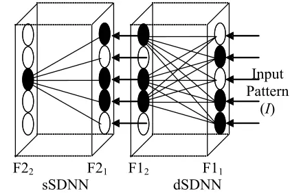
Figure 1: SDNN Architecture

2. The Snap-Drift Neural Network

(SDNN) and Modal Learning

The ideal of modal learning is that there are N modes of learning that the learning agent may select. This can be random, or performance guided. If it is performance guided the idea is to in effect maintain a list of modes, swapping between the front two modes unless one of them fails to improve performance over two selections in a row, in which case it goes to the back of the queue. In this simple case, with just two modes the toggling between them is controlled according to performance.

The modular neural network, modified from the performance-guided Adaptive Resonance Theory (P-ART) network first introduced by Lee and Palmer-Brown (Lee 2004a), is shown in Figure 1.

On presentation of an input pattern at the input layer F01, distributed SDNN (dSDNN)

will learn to group them according to their general features using snap-drift. In this case, the five F21 nodes (D = 5) whose

weight prototypes best match the current input pattern, are used as the input data to the selection SDNN (sSDNN) module for the purposes of feature classification. In both of the SDNN modules, the standard matching and reset mechanism of ART (Carpenter 1987, 1989) is discarded. Instead, in the dSDNN module, the output nodes with the highest net input are always

accepted as winners. In the sSDNN module, a quality assurance threshold is introduced. If the net input of a sSDNN node is above the threshold, the output node is accepted as the winner, otherwise a new uncommitted output node will be recruited as the winner and initialised with the current input pattern.

In this classifier version of SDNN, the performance is calculated separately for each sSDNN node, and is the proportion of times in which its activation as winner contributes to successful classifications. Together with the probabilistic aspect to enhance reinforcement and stability, introduced in (Lee, 2004b), the main purpose of node level performance calculation is to enable the sSDNN to retain the learning of nodes with successful adaptation, by continuing learning with the same learning mode if the node performance has increased since the last performance update. Alternatively, if the performance of a particular node decreased since the last epoch, or since the last epoch it was selected as a winner for learning of an input pattern, the learning mode of that particular sSDNN node will be swapped to the alternative learning node to encourage re-learning to occur in order to improve the performance of the node. This is also applied to the dSDNN nodes where the sSDNN inputs are generated. Thus, the learning mode of each of the sSDNN output nodes varies during each learning epoch. The following is a

Input Pattern

(I)

F11 F12

F21 F22

dSDNN (Feature Extraction) sSDNN

summary of the steps that occur in SDNN:

Step 1: Initialise parameters for each node: (α = 1, σ = 0), epochs = 500, D=5

Step 2: For each epoch (t)

Measure or calculate the performance of each sSDNN node over the last epoch, PsSDNN(t) Set probability of learning on that node, PL = 1 – PsSDNN (t)

Step 2.1: Find the D winning nodes at F12 with the largest net input.

Step 2.2: Process the output patterns of F12 as input pattern of F21.

Step 2.3: Find the node at F22 with the largest net input.

Step 2.4: Test the threshold condition:

IF (the net input of the node is greater than the threshold)

THEN

Test: Learning Mode Selection condition Weights of the dSDNN and sSDNN output nodes are adapted according to the Learning Mode Selection.

ELSE

An uncommitted sSDNN is selected and its weights are adapted with (α = 1, σ = 0).

Learning ModeSelection condition:

IF (PsSDNN(t) < PsSDNN(t - 1))

Weights of dSDNN and sSDNN output nodes are adapted with probability PL using the alternative learning procedure: (α,σ) becomes inverse(α,σ) for the node.

ELSE

Weights of dSDNN and sSDNN output nodes are adapted with probability PL, using the same learning procedure for the node as in epoch (t – 1): (α,σ).

3. The Snap-Drift Algorithm

The learning algorithm uses a novel combination of a modified form of Adaptive Resonance Theory (snap) (Carpenter, 1987a) and Learning Vector Quantisation

(drift) (Kohonen, 1990). In simple terms, the basis of the snap-drift weight update

algorithm can be stated as:

Snap-Drift=α(Fast_Learning_ART)+

σ(LVQ) (1) The top-down learning of both of the modules in the neural system is as follows:

wJi(new) = α(I ∩ wJi(old)) + σ(wJi(old) + β (I -

wJi(old))) (2) where wJi = top-down weights vectors; I = binary input vectors, and β = the drift speed constant = 0.5.

When α = 1, fast, minimalist (snap) learning is invoked:

wJi(new) = I ∩ wJi(old) (3) In contrast, when σ = 1, (2) simplifies to:

wJi(new) = wJi(old) + β (I - wJi(old)) (4) which causes a simple form of clustering at a speed determined by β. The bottom-up learning of the neural system is simply a normalised version of the top-down learning.

wiJ(new) = wJi(new) / | wJi(new)| (5) where wiJ(new) = top-down weights of the network after learning.

4. The SDNN Simulations

4.1 Lancaster Parsed Corpus (LPC):

The LPC is a corpus of English sentences and is a subset of the Lancaster/Oslo-Bergen Corpus (LOB). Each word is tagged with its syntactic category and each sentence in the LPC has undergone syntactic analysis in the form of labeled bracketing. In the simulations, a subset of samples from the LPC used in (Tepper, 2002) is adopted for the sake of comparison.

4.2 Input Representation:

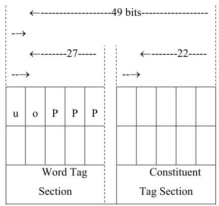
The design of the input patterns is according to the structure of the pre-tagged corpus (Garside, 1987). This is achieved by separating the input space into several regions where each corresponds to a different symbol type. For the input set used in SDNN, there are 9 groups of symbol type, represented by separate fields in the input vector.

A total of 49 bits are used to encode all the symbol types. The terminal symbol groups are: punctuation (Pu), conjunction (Co), nouns (NP), verbs (VP) and prepositions (PP). The non-terminal symbol groups are Sentences (S), Finite clauses (F), Non-finite clauses (T), major phrase types (V) and minor phrase types (M). Together with 4

Look Back symbols and 1 Look Ahead

symbol (Tepper, 2002), this makes the total number of input fields = 15. By using linear binary coding for each symbol type within each input field, the input size of the SDNN is 49 x 15 = 735. With the available Pre-tagged sentences in, we generate 254 input patterns, from all stages of parsing, typically involving mixtures of terminal and non-terminal symbols.

4.3 Training and Test Inputs

Half of the input set (127) is used to train the SDNN. During each epoch, 10 input patterns out of the 127 training inputs are randomly selected after which the performance of each sSDNN node and overall system performance are calculated. After 500 epochs, the SDNN is tested.

There are 2 types of test input: Natural Test inputs, consist of a mixture of training and new input patterns that SDNN never encountered before (154 patterns); and Pure

test data, which consists only of input

patterns that SDNN has never encountered before (89 patterns). Table 1 shows the number of input patterns for each symbol type.

4.4 Simulation 1: Results and Discussions

In simulation 1, we looked at the average performance improvement that can be achieved by using the whole set of available input patterns to train the SDNN. Table 2 shows the results of the simulation, where it is shown that after just 150 epochs, SDNN is able to achieve an average performance of 75%, and after ~300 training epochs, SDNN has achieved an overall performance of average 94%, and has converged.

4.5 Comparisons between Snap-Drift and MLP with Back-Propagation

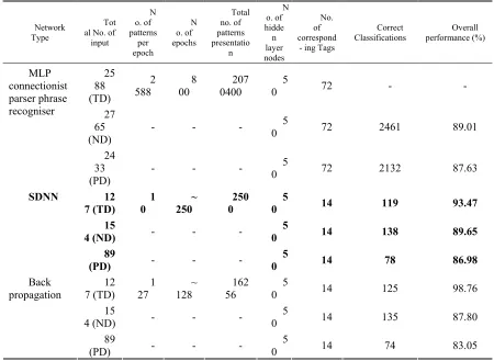
Table 1 shows the comparison between the results from the MLP connectionist parser phrase recognizer, the SDNN, and a simple back-propagation network.

←---49 bits---

-→

← ---27---→

← ---22---→

u o P P P

Word Tag Section

Constituent Tag Section

Network Type

Tot al No. of input N o. of patterns per epoch N o. of epochs Total no. of patterns presentatio n N o. of hidde n layer nodes No. of correspond

- ing Tags

Correct Classifications Overall performance (%) 25 88 (TD) 2

588 00 8 0400 207 0 5 72 - -

27 65

(ND) - - -

5

0 72 2461 89.01

MLP connectionist parser phrase recogniser 24 33

(PD) - - -

5

0 72 2132 87.63

12 7 (TD) 1 0 ~ 250 250 0 5

0 14 119 93.47

15

4 (ND) - - -

5

0 14 138 89.65

SDNN

89

(PD) - - -

5

0 14 78 86.98

12

7 (TD) 27 1 128 ~ 56 162 0 5 14 125 98.76

15

4 (ND) - - - 0 5 14 135 87.80

Back propagation

89

(PD) - - - 0 5 14 74 83.05

Table 1

The results from each of the neural networks can be divided into 3: results during training (TD), results from testing using Natural test data (ND) and results from testing using just

Pure test data (PD). By comparing the results between SDNN and a simple back-propagation network, with both using the same set of data, we can see that SDNN has obvious advantages in the speed of learning. During training, the SDNN network only required 2500 randomly selected training

data to achieve a performance of 93%, whilst back-propagation required 6 times the number of input presentations to achieve performance of 98%. During testing, SDNN correctly classifies 4 more patterns than MLP, This is not a clearly statistically significant difference in performance, but it is, taken over many simulations, clear evidence of comparable performance between the two approaches.

Furthermore, the main reason why SDNN and the backpropagation network are unable to achieve maximum performance is mainly to do with the number of input patterns for each of the symbols, which varies greatly and is insufficient in some cases. For

unsurprisingly they tend to be recognized as S.

If we compare SDNN results with the MLP connectionist parser phrase recognizer that uses a much larger set of inputs, 20 times larger than the one used by SDNN, that phrase recognizer required 100 times more input presentations which is about 5 times more for each input pattern to be learnt.

5. Conclusions and Future Work

In conclusion, the snap-drift algorithm has shown potential in phrase recognition. The results show the learning of the SDNN is fast, stable and reliable in recognizing the input patterns and is able to group them according to their internal structure. This is still the preliminary stage of the research into this application, but comparisons with results achieved by an MLP with back-propagation on the same task have shown that SDNN has the right dynamics and capability to equal if not better the MLP and at a higher speed. The next stage will be applying SDNN with a larger set of input patterns to see how it scales up in this task.

References

Carpenter, G., Grossberg, S., “ A Massively Parallel Architecture for a Self-Organising Neural Pattern Recognition Machine”,

Computer Vision, Graphics and Image Processing, 1987, Vol. 37, pp. 54 – 115.

Carpenter, G., Grossberg, S., “Search Mechanism for Adaptive Resonance Theory (ART) Architecture”, Proceeding of IJCNN, 1989, Vol. I, pp. 201 – 205.

Donelan, H., Pattinson, C., Palmer-Brown, D., Lee, S. W., “The Analysis of Network Manager’s Behaviour using Self-organising

Neural Network”, Proceeding of ESM, Magdeburg, Germany, 2004, pp. 111 – 116.

Garside, R., Leech, G., Varadi, T., Manual of Information to Accompany the Lancaster Parsed Corpus, University of Oslo, 1987.

Kohonen, T., “Improved Versions of Learning Vector Quantization”, Proceeding of IJCNN, 1990, Vol.1, pp. 545 – 550.

Lee, S. W., Palmer-Brown, D., Tepper, J., Roadknight, C. M., “Snap-Drift: Real-time Performance-guided Learning”, Proceeding of IJCNN, Portland Oregon, 2003, Vol. 2, pp. 1412 – 1416.

Lee, S. W., Palmer-Brown, D., Roadknight, C. M., “Performance-guided Neural Network for Rapidly Self-Organising Active Network Management”, Neurocomputing, Elsevier, 2004a, Vol. 61C, pp. 5 – 20.

Lee, S. W., Palmer-Brown, D., Roadknight, C. M., “Reinforced Snap-Drift Learning for Proxylet Selection in Active Computer Networks”, Proceeding of IJCNN, Budapest, 2004b, Vol. 2, pp. 1545 – 1550.

Marshall, R., Mayberry, III. Risto, M., “SARDSRN: A Neural Network Shift-Reduce Parser”, Proceeding of the 16th IJCAI, Stockholm, Sweden, 1999, pp. 820 – 825.

Rushton, J. N., “Natural Language Parsing using Simple Neural Networks”, Proceeding of ICAI, 2003.