Department
of Statistics
Detecting Semi-plausible
Response Patterns
by
Tayfun Terzi
A thesis presented for the degree of
Doctor of Philosophy
in the subject of
Statistics
Declaration
I certify that the thesis I have presented for examination for the PhD degree of the London School of Economics and Political Science is solely my own work other than where I have clearly indicated that it is the work of others (in which case the extent of any work carried out jointly by me and any other person is clearly identified in it).
The copyright of this thesis rests with the author. Quotation from it is permitted, provided that full acknowledgement is made. This thesis may not be reproduced without my prior written consent.
I warrant that this authorisation does not, to the best of my belief, infringe the rights of any third party.
Acknowledgements
First and foremost, I would like to thank my supervisors Professor Chris Skin-ner CBE and Dr Jouni Kuha for offering invaluable advice, their guidance, their contribution of time, as well as the space and freedom I was granted and entrusted with. It was Chris’ inspiring intuition and expertise, his very contagious calmness, and his belief in me that gave me the energy to excel in my work. I feel honoured that I was given the chance to prove myself under the supervision of one of the most eminent and distinguished experts in the field. It was Jouni’s intellectual brilliance and knowledge (in fact, I personally will never stop believing that he knows everything, even though he would humbly deny that statement), his patience, and his unprecedented time commitment as my second supervisor that made me tirelessly challenge but not doubt myself.
Second, I would like to extend my sincerest thanks to Dr Jason Huang and Professor John A. Johnson for allowing me to use their questionnaire data. The datasets were of paramount importance in evaluating the findings of this thesis and provided an excellent platform for the formation of ideas.
Third, I gratefully acknowledge the Economics and Social Research Council and the London School of Economics and Political Science for providing the funding which allowed me to undertake this research. Particularly, I would like to thank the administration staff at the Department of Statistics for not only just doing their jobs but far more for their almost parental dedication towards improving their PhD students’ experiences at LSE.
Fourth, I would like to express my gratitudes to Professor Irini Moustaki and Professor Joop Hox who are honouring me by acting as my examiners in my viva voce examination. There is no greater reward for a finishing PhD student than to discuss our lifetime achievement with researchers to whom we look up to and whose opinion we value and respect.
beautiful moments we have shared in the second-floor office of the Columbia House are unforgettable memories and moments, which I will dearly miss.
Abstract
New challenges concerning bias from measurement error have arisen due to the increasing use of paid participants: semi-plausible response patterns (SpRPs). SpRPs result when participants only superficially process the information of (online) experiments/questionnaires and attempt only to respond in a plausible way. This is due to the fact that participants who are paid are generally motivated by fast cash, and try to efficiently overcome objective plausibility checks and process other items only superficially, if at all. Thus, those participants produce not only useless but detrimental data, because they attempt to conceal their malpractice. The potential consequences are biased estimation and misleading statistical inference.
Contents
1 Introduction 16
1.1 Primary Source: Micro-Jobbers . . . 18
1.2 Semi-plausible Response Patterns . . . 21
1.3 Thesis Outline . . . 26
2 Review of Methods for Detection 29 2.1 Identification Measures . . . 30
2.1.1 Measures for (theory-driven) Outlier Detection . . . 31
2.1.2 Person-Fit for categorical Variables . . . 37
2.1.3 Person-Fit for continuous Variables . . . 46
2.1.4 Conclusions from the Review . . . 49
2.2 Latent Class Approach . . . 50
3 Empirical Data and the basic Latent Variable Model 57 3.1 The Big Five Personality Factors . . . 57
3.2 Investigated Datasets . . . 59
3.2.1 Assessment Instrument . . . 59
3.2.2 Experimental Study (Huang et al., 2012) . . . 59
3.2.3 Online Questionnaire (Johnson, 2005) . . . 62
3.3 Analysis assuming valid Responses only . . . 62
3.3.1 Theoretical Model . . . 62
3.3.2 Descriptive Statistics . . . 67
3.3.3 Goodness of Fit . . . 76
3.3.4 Parameter Estimates . . . 80
4 A Latent Class Model accommodating invalid Responses 86
4.1 Multi-Group and Latent Class Models . . . 86
4.1.1 The Multi-Group Model . . . 87
4.1.2 Independence of Construct(s) of Interest and invalid Responses 88 4.1.3 Diversity of invalid Responders . . . 89
4.1.4 Conditional Independence and Method Factors . . . 90
4.2 A Model incorporating a Method Factor . . . 91
4.3 Computational Implementation . . . 95
4.4 Comparing the different Analysis Results . . . 98
4.5 Predicted Class Membership . . . 107
4.6 Discussion . . . 110
5 A new Measure for Detection 112 5.1 Modifying the Covariance-based Index . . . 112
5.1.1 Maximum Penalty Conditions . . . 112
5.1.2 Key Quantities . . . 115
5.2 Methods for Detection using the new Measure . . . 124
5.2.1 Information Sources for Ti . . . 124
5.2.2 Deriving Cut-off Values for Ti . . . 126
5.2.3 Summary . . . 128
5.3 Motivation for the Modification with empirical Data . . . 129
5.3.1 Distributional Properties . . . 129
5.3.2 Comparing Results of original and modified Versions . . . 135
5.4 Deriving the theoretical Distribution . . . 141
6 Evaluation of the new Measure 150 6.1 Numerical Example using Latent Class Response Models . . . 151
6.1.1 Valid Responses under the valid Response Model . . . 151
6.1.2 Valid and invalid Responses under the valid Response Model . 156 6.1.3 Valid and invalid Responses under the biased valid Response Model . . . 162
7 A Simulation Study 172
7.1 Simulation Conditions . . . 173
7.1.1 Theoretical Models . . . 173
7.1.2 Samples . . . 178
7.2 Evaluation Scenarios . . . 179
7.3 Classification Results . . . 180
7.3.1 Theoretical Ti Parameters and theoretical Percentiles . . . 180
7.3.2 Estimated Ti Parameters and theoretical Percentiles . . . 182
7.3.3 Estimated Ti Parameters and estimated Percentiles . . . 184
7.4 Further Results and Implications . . . 187
7.4.1 Discriminatory Potential . . . 188
7.4.2 Risk of extreme valid Response Values . . . 189
8 Discussion 192 Bibliography 198 A Tables 217 A.1 Reviewed Person-Fit Indices . . . 217
A.2 Empirical Results with translated Percentages . . . 219
A.3 Comparing Parameter Estimates of several Models . . . 220
A.4 Simulation Results with translated Percentages . . . 222
List of Tables
2.1 Values ofGias simplified index withωj = γj for four example response
patternsxi of participants i given γ . . . 40
3.1 Instructions . . . 60
3.2 Sub-samples . . . 61
3.3 Parameter notations and labels related to the three latent variables . 64
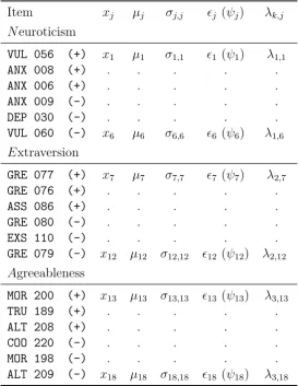
3.4 List of IPIP observed variables as indicators for the three latent variables 66
3.5 Mean and standard deviations of observed variables’ means and stand-ard deviations for the sub-groups of the experimental study and online questionnaire samples . . . 75
3.6 Model fit indices for different samples assuming valid responses only . 78
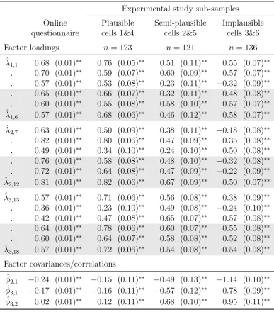
3.7 Parameter estimates and standard errors for different samples . . . . 83
3.8 Absolute differences between parameter estimates of different samples summarised for different types of parameters . . . 84
4.1 Model fit indices for the latent variable and latent class model for two different samples . . . 101
4.2 Model fit comparison indices for two study samples . . . 102
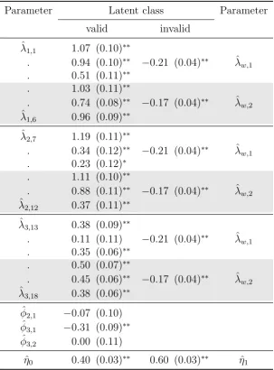
4.3 Two-class model parameter estimates and standard errors for the experimental study sample . . . 103
4.4 Means of explained variances based on observed variables’ factor loadings on either of the three factors for the valid response model in the latent variable versus latent class model . . . 106
4.6 2x2 count table of predicted latent class versus experimentally induced/ observed sub-sample membership . . . 109
5.1 Results of the binary-logistic regression of experimental study sub-sample membership on three contrast components, where parameters for the contrast components are estimated using different samples (evaluation scenarios) . . . 137
5.2 Percentage of correctly classified semi/-implausible sub-sample mem-bers of the experimental study sample, where parameters for iden-tification measure are estimated using different samples (evaluation scenarios) . . . 139
5.3 Percentage of sub-sample members of the experimental study sample identified as extreme values in Υi(N,Σ), where parameters for Υi(N,Σ)
are estimated based on different samples (evaluation scenarios) . . . . 140
6.1 Empirical and theoretical percentiles of Ti for valid responses under
the theoretical valid response model . . . 153
6.2 Empirical and theoretical expected value and variance of Ti for valid
responses under the theoretical valid response model . . . 154
6.3 Percentage of responders identified as extreme values using the theor-etical percentiles as cut-off values for each response group separately . 157
6.4 Empirical mean and variance for estimated factor scores based on the theoretical valid response model for valid and invalid (item wording) response groups . . . 158
6.5 Empirical mean and variances for Ti and its components for valid and
invalid (item wording) response groups . . . 158
6.6 Correlations between components of Ti within valid response and
invalid response groups . . . 161
6.7 Correlations between components of Ti within valid response and
invalid response groups . . . 161
6.8 Percentage of responders identified as extreme values using the theor-etical percentiles as cut-off values for the two response groups separately164
6.10 Percentages of respondents in experimental study sub-samples flagged as extreme values with cut-off defined by estimated 5th and 95th
percentiles ofTi based on different information sources as estimates
for the valid response model . . . 167
6.11 Percentages of respondents in experimental study sub-samples flagged as extreme values with cut-off defined by estimated 1st and 99th
percentiles ofTi based on different information sources as estimates
for the valid response model . . . 168
7.1 Specifications of the valid response population models . . . 174
7.2 Percentage of simulated responses in the groups valid, item wording, and long string identified as extreme values averaged throughout all simulation conditions and replications within conditions, separately presented for different conditions of a priori defined average percentage of error variance in the valid response population model (simulation study evaluation scenario: theoretical parameters and theoretical percentiles) . . . 181
7.3 Percentage of simulated responses in the groups valid, item wording, and long string identified as extreme values averaged throughout all simulation conditions and replications within conditions, separately presented for different conditions of a priori defined average percentage of error variance in the valid response population model and altern-ated percentage of valid responders in the sample (simulation study evaluation scenario: estimated parameters and theoretical percentiles) 183
7.5 Multiple regression coefficients - sub-sample: simulation conditions with 25% error variance - dependent variable: percentage of extreme Ti values of invalid responders - predictors: simulation condition factors188
7.6 Multiple regression coefficients - dependent variable: percentage of extremeTivalues of valid responders - predictors: simulation condition
factors . . . 190
A.1 Categories of popular person-fit indices and their feasibility under non-parametric (descriptive) and binary-logistic model approaches (under IRT terminology: Rasch model, two-parameter-logistic, and
three-parameter-logistic model) . . . 218
A.2 Number of sub-sample members of the experimental study sample iden-tified as extreme values in Υi(N,Σ), where parameters for Υi(N,Σ)
are estimated based on different samples (see correspondingTable 5.3)219
A.3 Parameters estimates and standard errors for different samples based on different models . . . 221
A.4 Numbers of simulated responses identified as extreme values translated from percentages reported inTable 7.4 based on corresponding sub-sample sizes of respective simulation conditions (simulation study evaluation scenario: estimated parameters and estimated percentiles) 223
List of Figures
1.1 A meta-theory of response validity, involved processes, and resulting data plausibility for exemplary response strategies. . . 23
2.1 Illustrative example for the Mahalanobis distance, for two response patterns labelled a and b. . . 37
2.2 Illustrative example of the individual log-likelihood contribution `i(θ),
for two response patterns labelled a and b. . . 44
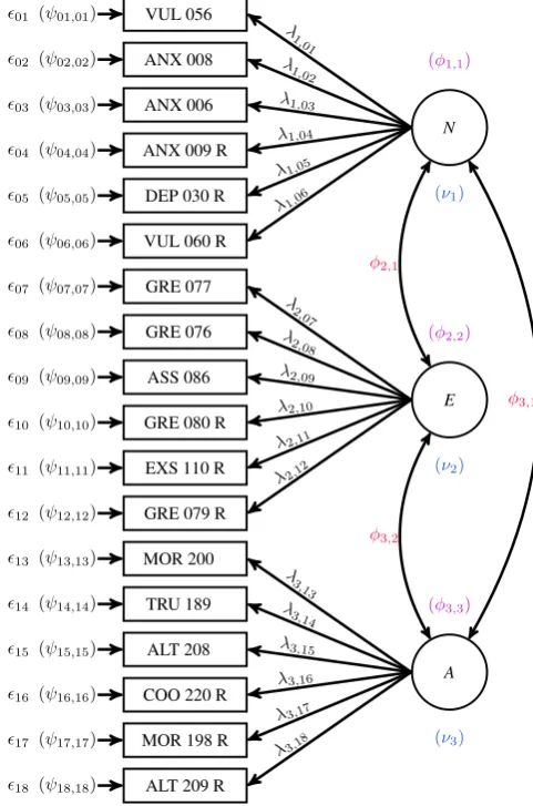
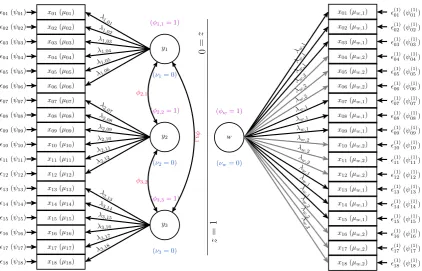
3.1 Path diagram for the Big Three factor model. . . 67
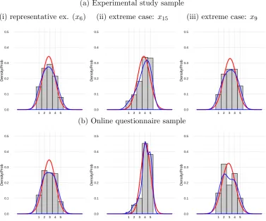
3.2 Histograms for a representative observed variable (i) and selected observed variables which are the two extreme cases (ii) and (iii), for the experimental study and online questionnaire samples with their corresponding normal density curves and kernel density estimates. . . 71
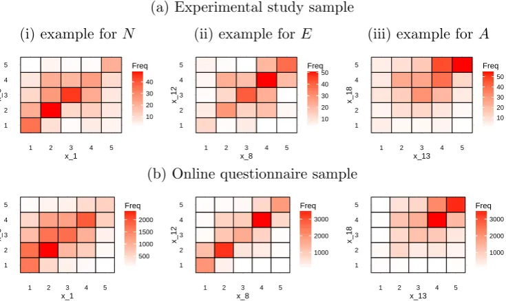
3.3 Bivariate mosaic plots for example indicator variables for each latent variable, for the experimental study and online questionnaire samples, where cell frequencies are represented by colours (heat map). . . 73
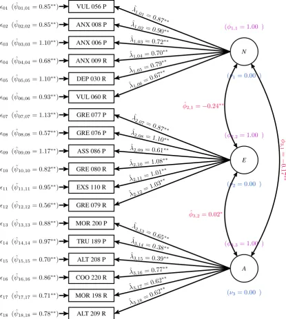
3.4 QQ-Plots for the Mahalanobis distance for the experimental study sample, the plausible response sub-sample and online questionnaire sample against the theoretical χ2(18) distribution . . . . 73 3.5 Big Three factors model path diagram with parameter estimates for
the online questionnaire sample. . . 81
5.1 Possible contrast components ordered with respect to model restrict-iveness. . . 114
5.2 Stacked histogram based on class/group membership for D2
i(Σ) for
online questionnaire sample (top) and experimental study sample (bottom) with the correspondingχ2 distribution curve. . . . 130 5.3 Stacked histogram for D2
i(N) for online questionnaire sample (top)
and experimental study sample (bottom). . . 132
5.4 Stacked histogram for Υi(N,Σ) for online questionnaire sample (top)
and experimental study sample (bottom). . . 133
5.5 Stacked histogram for Υi(Σ, S) for online questionnaire sample (top)
and experimental study sample (bottom). . . 134
6.1 Kernel density estimates of Ti for valid responses based on the
ran-domly drawn valid response model sample. . . 152
6.2 Cumulative distribution of Ti based on the randomly drawn valid
response model sample and theoretical cumulative function based on parameters γ. . . 153
6.3 Kernel density estimates for all components of Ti for valid responses
under the theoretical valid response model defined by the valid class of the latent class analysis estimated for the online questionnaire study sample. . . 155
6.4 Kernel density estimates of Ti for valid responses (dashed/dotted
curve) and two types of invalid responses (item wording and long string) when theoretical model for valid responders is known. . . 157
6.5 Kernel density estimates for components of Ti under the alternative
representation for invalid responses under the theoretical valid response model defined by the valid class of the latent class analysis estimated for the online questionnaire study sample. . . 160
6.7 Kernel density estimates of Ti for valid responses and invalid responses
(of type item wording) when we have biased estimates of the theoretical model for valid responses and a reference curve for valid responses when the theoretical model is known (dashed/dotted curve). . . 163
6.8 Histograms for values of Ti presented in dodged form for the
experi-mental study sub-samples semi-/implausible (in grey) and valid (in black) with corresponding estimates of 1st and 99th percentiles
indic-ated as dashed/dotted vertical lines for different evaluation scenarios. 170
Chapter 1
Introduction
With the recent rise of new possibilities in research regarding a new form of online recruiting where people are paid to act as participants, the challenge for eliminating response biases through statistical analysis has become more important. Researchers anticipate that those tools which rely on online recruited and paid participants will soon become an important tool for research in many social disciplines (e.g., Mason and Watts, 2009; Buhrmester, Kwang, and Gosling,2011). Hence, there is an increased need for the evaluation of implications associated with the usage of paid participant pools.
I argue that one of the worrying implications areSemi-plausible Response Patterns
(SpRPs), which result when participants superficially process the information of (online) experiments or questionnaires and try only to respond in a plausible way. This is due to the fact that participants who are paid are generally interested in earning fast money and efficiently attempt to overcome objective plausibility checks, and process all other items only superficially, if they process them at all. Thus, those people produce not only useless but detrimental data, because they attempt to conceal their malpractice from the ”employer”, or rather the test administrator. The consequences of this new increase in measurement error are biased estimation and blurred or even covered true effect sizes, which contaminate valid models (cf. Mavridis and Moustaki, 2008, 2009).
‘subtle yet insidious threat to data quality [. . . ]’ (2012, p. 100). While Huang et al. (2012) use the label insufficient effort responding (IER), others refer to this type
of responding as random (Beach, 1989; Berry et al.,1992),careless and inattentive
(e.g., Curran, Kotrba, and Denison, 2010; Meade and Craig, 2012), or inconsistent responding (McGrath, Mitchell, Kim, and Hough, 2010), also terms like content
nonresponsivity (Nichols, Greene, and Schmolck, 1989),protocol invalidity (Johnson,
2005) and speeders (Greszki, Meyer, and Schoen, 2014) are often used. The foci lie on different causes (e.g., lack of motivation) and contexts (e.g., online vs. paper-and-pencil survey) leading to different labels of types of responding. In spite of different labels, these situations are also leading to fundamentally similar response patterns. Many of these constructs overlap in the idea that participants respond without (any) regard to item content (see Section 1.2 for a detailed distinction). Identifying those response patterns could help to improve the criterion-related validity of measure (McGrath et al., 2010). Couch and Keniston (1960) already stated that these kinds of undesired response patterns should either be treated as outliers (e.g., by controlling for them or removing them from the sample) or they should be seen as manifestations of participants’ characteristics.
SpRPs are particularly characterised by the idea that participants do not respond entirely without regard to item content, but rather try to respond in a way that the researcher will not easily detect. This kind of semi-plausible responding is what renders SpRPs a special and more severe version of invalid protocols.
A researcher is confronted with three questions:
• How to prevent or at least minimise SpRPs? • How to recognise those SpRPs?
• How to deal with biased estimates of any quantity due to SpRPs?
responses are by definition not easily identifiable as merely rare or extreme responses without taking a broader context into account. Other efforts towards capturing measurement error and increasing the reliability of measurements are often very effective, but rarely applicable for systematic measurement error or measurement error that is not produced by everyone in the sample but rather a small group of people. Thus, in the case of SpRPs, comparing response patterns as a whole with plausible response patterns could help with classifying them as valid or invalid protocols. Starting points are procedures such as person-fit indices (Meijer and Sijtsma, 2001) which identify the extent to which a response pattern deviates from the latent model. Measures in areas dealing with non-response bias and missing data (Allison, 2009) can also be drawn upon for the treatment of SpRPs.
In this thesis, I will identify primary sources of SpRPs, discuss their consequences and establish a theoretical framework linked to other already well-established research areas. This will be followed by a literature review of available identification indices developed for different kinds of undesired response patterns. By drawing upon an experimental dataset as well as largely implemented data on an empirically well-investigated framework of the Big Five personality factors, I will examine statistical properties of SpRPs. Ultimately, this will help to establish a statistical theory of SpRPs with the focus on latent variable models in order to develop and evaluate an optimal, universally applicable identification measure. The thesis will conclude with a brief discussion about attempts to deal with SpRPs, once they are identified.
1.1
Primary Source: Micro-Jobbers
In this section, I will set out the primary source of SpRPs. Although the potential for generalisability of results to other sources will be discussed throughout the thesis, the reader should be aware that micro-jobbers introduced in this section serve as the group of focus.
100 countries. This is a diverse potential participants pool available for many kinds of surveys or experiments. However as the term labour already implies, money plays the central role for this work force’s motivation to attend as participants. It is essential that the labour commissioner can refuse payment if the work is not done properly, e.g. the participant has not completed the questionnaire in a way a researcher has expected him or her to do. Furthermore, these monetary compensations are typically small. A review of MTurk (Mason and Suri,2012) but also other reviews of general micro jobber platforms (Buhrmester et al., 2011) report only very small amounts of money such as five to ten cents (USD) for 5 to 10-minute tasks. Paolacci, Chandler, and Ipeirotis (2010) used those platforms to replicate classic studies at a cost of approximately $1.71 per hour per subject.
Another reason why a growing number of researchers make use of micro-jobber platforms besides the low cost is that it is supposed to reduce certain kinds of biases found in traditional samples (Gosling, Vazire, Srivastava, and John, 2004). It is argued that the samples in internet surveys consist of demographically more diverse participants than typical college samples (e.g., in the US, Germany and other countries) broadening the validity beyond undergraduate students (Eriksson and Simpson, 2010). Conducting experiments also appears to be time-saving, allowing for faster cycles with regards to continuously updating of methodology and theory (Mason and Suri, 2012). Concerning the validity of provided responses, Buhrmester et al. (2011) reports satisfying results in terms of psychometric standards based on participants recruited in this manner. However, one cannot deny that a sample consisting of micro-jobbers is a sample of individuals mainly seeking to earn money. It is hard to believe in data provided by Buhrmester et al. (2011) in his brief and very positive review of MTurk which reports participants to be internally motivated (e.g., for enjoyment).
and given their reported high income per annum. The most important driver for MTurk workers is reported to be the monetary outcome. Only 12% of U.S. worker report that MTurk money is irrelevant for them. However, Ipeirotis (2010, cited in Mason and Suri, 2012) states that the vast majority see MTurk also as a fruitful way to spend free time while earning some cash. Nonetheless, nearly 10 % also seem to scrape together a living using MTurk.
Caveats of using online questionnaires are diverse. One major disadvantage is that researchers often are required to deal with duplicates. This means that some individuals might complete an online questionnaire or experiment several times using multiple identities. Although this is partly controlled using browser cookies and tracking IP addresses, experienced users circumvent these and efficiently produce detrimental data. Another problem is the use of software programs or so-called bots
that complete questionnaires.
Even more concerning, in terms of cursory detecting invalid responders, are individuals who attempt to make as much money as quickly as possible without regard to the instructions or intentions of the study. Mason and Suri (2012) and others refer to those participants as spammers. Spammers especially target surveys, since these are easy to complete. This is often done in a random but more predominantly in a semi-plausible manner, since bogus items are often implemented in these surveys to identify obviously implausible responders. Semi-plausible/undetectable response patterns are more popular as these less often lead to a refusal of payment, which would, in turn, lead to a bad reputation of this worker on platforms where these kinds of mechanisms are implemented. Furthermore, although the number of these kinds of workers might not be large, the data, and thus the participant entries they produce, are severely detrimental for the subsequent analysis of data.
I primarily focus on paid mass participants because the prevalence of invalid responders is expected to be most severe and invalid response strategies more successfully concealed in these scenarios. However, findings of this thesis are easily generalisable to other settings. Miller (2006) reported in a study of 13 US panels that about 5-10% of participants responded to obvious plausibility checks (also referred to
as red herring questions) incorrectly, indicating the use of invalid response strategies.
long string response strategy), thus, not even trying to hide their intentions (cited from Greszki et al., 2014). Meade and Craig (2012) used 11 different identification measures and concluded that 5-15% of participants in undergraduate internet surveys lack sufficient attention. Further analysis using factor mixture model analyses also indicated that around 10 to 12% of their undergraduate sample belonged to alatent
class that can be considered careless in their responses, which is nearly identical
to results reported by Kurtz and Parrish (2001). Woods (2006) has found that in certain (commonly encountered) scenarios it only requires 1% to 20% of careless responses in the sample for models not to fit the data anymore.
1.2
Semi-plausible Response Patterns
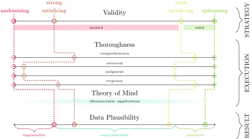
Having set out the primary source and the subject of this thesis, I will continue to discuss causes of SpRPs from a cognitive psychological perspective. In doing so, I seek to define the terminology used throughout the thesis at hand, and depict links to other constructs in the literature. The meta framework, illustrated in Figure 1.1, seeks to capture these links between concepts of response strategy, the cognitive processes involved and on the other hand the actual resulting plausibility of data. Links between response validity, involved cognitive processes, and data plausibility of shown (invalid) response strategies are conceptual examples.
In his prominent review of survey research, Krosnick (1999) states that there is wide agreement about the cognitive processes that result in valid response patterns (e.g., Cannell, Miller, and Oksenberg, 1981; Schwarz and Strack,1985; Tourangeau and Rasinski, 1988). Kahn and Cannell (1957) discuss in detail the so-calledcognitive
process model based on the original work of Tourangeau (e.g., Tourangeau, Couper,
and Conrad, 2000; Tourangeau, 1984, 1987). Valid respondents answer questions properly when they, first, read the entire question text to comprehend, interpreting the question and deducing its intent (P1). Secondly, valid response patterns require accessing relevant information in a participant’s memory (P2). Thirdly, based on accessible information, a (single) subjective judgement is formed (P3). Lastly, participants then formulate or translate that judgment into a response, e.g. selecting an answer option based on offered alternatives (P4).
Fabrigar, 2001). We can assume that if that applies to a single question, it applies even more to a large number of observed variables. We can represent the thoroughness of their execution on individual scales as drawn in Figure 1.1. Psychology of survey participants considers several aspects that lead to this expenditure of cognitive effort (see Warwick and Lininger,1975): Participants might be motivated by desires for
self-expression, intellectual challenge, self-understanding, altruistic feelings or emotional catharsis. Krosnick (1999) further states that motives might include desires for gratification from successful performance to help the survey purpose (e.g., to help an administrator improve working conditions). These motives can be categorised under the psychological concept of intrinsic motivation (for a recent review about intrinsic versus extrinsic motivation, see Ryan and Deci, 2000). As the most mobilising form of motivation, it can easily be considered strong enough to facilitate a valid response. Nevertheless, we cannot always assume that participants are purely intrinsic but rather extrinsically motivated, for instance, driven through automatic compliance processes (e.g., Cialdini, 1993) or as students attempting to collect course credits. Sometimes motivation might even change throughout the course of the questionnaire when participants satisfy their desires to provide valid responses after answering a few questions, and become increasingly fatigued and distracted with each additional assessment. Unfortunately, usual sources of extrinsic motivation in surveys cannot be considered as secure paths for valid response patterns. Krosnick (1991) argues that participants might resolve this dilemma, which is a lack of intrinsic motivation and ineffective extrinsic motivation, by shifting to an invalid response strategy, compromising response standards and expending less energy.
The actual extent to which a response is valid can, apart from a binary classifica-tion, be located on a validity continuum as is shown in Figure 1.1. The valid anchor at the positive end of the continuum is often referred to as optimising (e.g., Krosnick,
1999). The actual position on the continuum then indicates the combined degrees of thoroughness executed throughout steps P1 to P4. A response strategy on the continuum not far from valid responses isweak satisficing (Simon,1957). This occurs when responses are the result of the complete but less than fully diligent execution of P1 to P4. Hence, participants settle for a merely satisfactory rather than a thoroughly processed answer. Yet another approach on the continuum might be referred to as
comprehension
retrieval
judgment
response
Thoroughness
invalid valid
Validity
STRA
TEGY
idiosyncratic application
Theory of Mind EXECUTION
Data Plausibility
implausible semi-plausible plausible RESUL
T
optimising weak
satisficing strong
satisficing
[image:23.595.124.540.104.333.2]randomising
Figure 1.1: A meta-theory of response validity, involved processes, and resulting data plausibility for exemplary response strategies.
literally. Following Neuringer (1986, p. 63), humans can learn to behave randomly, but they do not have the natural ability to do so (for reviews Tune, 1964a, 1964b; Wagenaar, 1972). Hence, participants who try to respond in a random manner will produce correlated responses, following some idiosyncratic, systematic way of ‘random’ responses. This is an important aspect because otherwise statistically random responses (independent responses following a uniform distribution) can to a certain extent be incorporated as random measurement error using latent variable frameworks (Medsker, 1994; Shook, Ketchen, Hult, and Kacmar, 2004). However, even such purely random measurement error would certainly have a bad impact on estimation, if it is completely unrelated to the respondent’s true position.
There are numerous methods we might employ with regards to questionnaire design or at data collection stage to minimise the occurrence of SpRPs. For example, we can reduce the perceived cost, such as perceived energy expenditure, by estab-lishing an intrinsically motivating instruction. A balance between monotony and standardisation of question design is very important. A monotone question design can easily lead to boredom. However, if questions do not follow a minimal common standard, cognitive processes require more capacity to adapt to different question formats. In general, a large number of questions should be avoided. Questions should focus on easily accessible memory and allow for additional answer options, such as a ‘don’t know’ answer option. There is a vast and rich range of literature on how to improve data quality, integrity, and response rate, simultaneously. As this thesis primarily seeks to develop and discuss measures to deal with SpRPs after data collection, I would like to refer the reader at this point to standard textbooks on survey methodology and online questionnaires (e.g., Leeuw, Hox, and Dillman,
2008).
ourselves (e.g., Baron-Cohen, 1991). Different processes either developed through social interaction or inferred from introspection enable healthy subjects to develop a theory of mind about the actual intentions of a question. In Figure 1.1, the theory of mind is represented as an additional cognitive variable that reduces validity but, in contrast, might increase data plausibility. Participants can employ an invalid response strategy based upon less cognitively exhausting question-cue-stimulus-response rules and yet produce response patterns that seem plausible from a quantitative data point of view.
Therefore, I introduce the concept of semi-plausible response patterns in order to emphasise that the investigative nature of this thesis focuses on the produced data. Semi-plausible and implausible response patterns are defined through their statistical nature in reference to the valid response model. This is in contrast to the processes and causes of invalid response strategies, which may or may not result in semi-plausible response patterns. For instance inFigure 1.1, we can see that weak and strong satisficing or even randomising can lead to semi-plausible response patterns. As another example, a long string response strategy can depending on features of the valid response model, create an easily detectable implausible response pattern. However, straight-lining might as well result in a semi-plausible response pattern where it is unclear whether the data is based on valid responses. Consequently, the notion ofsemi-plausible response patterns also indicates the difficulty in detecting invalid responses.
1.3
Thesis Outline
In the previous sections, I motivated and introduced SpRPs as a new problem and, hence, not exhaustively researched topic. I further defined SpRPs as the construct of interest within a framework of existing literature.
In this thesis, I seek to address problems arising from SpRPs and research on solutions to deal with them. In general, I propose two methods to deal with SpRPs, namely, accommodating semi-plausible response strategies into the statistical model and/or using identification measures for the detection of invalid responses to exclude them from further analyses. Methods developed within this thesis will be evaluated on two empirical datasets; one being an experimental study and the other an online questionnaire study. Furthermore, a large-scale simulation study will be conducted such that we can identify relevant information to the prediction of success scenarios in separating valid from invalid responders.
In Chapter 2, detection methods from existing literature will be introduced and reviewed. I will discuss identification measure from other relevant fields such as cheating and fraud detection. This knowledge will serve as an example for the development of an appropriate test measure for the detection of SpRPs. Furthermore, I will draw on latent class analysis as a statistical tool for the accommodation of invalid response strategies. Previous implementations of latent class models in related studies will serve as examples for the definition of an appropriate framework to reduce measurement error from SpRPs.
interest.
In Chapter 4, the traditional latent variable analysis model will be extended to accommodate a latent class for invalid responders. I will propose and analyse an example latent class model that accounts for one type of possible invalid response strategies. This method will be evaluated in three ways. First, model fit test statistics and indices will be compared between the latent class analysis and traditional latent variable analysis results. Secondly, individual parameter estimates are going to be assessed based on whether accommodating an invalid response strategy helps to reduce measurement error and estimation bias. Lastly, based on the posterior distribution of the latent class variable, response patterns will be assigned to either class to evaluate the success of correctly assigning plausible response patterns to the valid response class and semi/-implausible response patterns to the invalid response class.
In Chapter 5, I will motivate, derive, and discuss a new test statistic for the identification of SpRPs. The new measure is a modified version of an existing identification measure and will be interpreted within the framework of latent variable models followed by a discussion of possible application methods. The modification will be further motivated by comparing its performance in detecting semi/-implausible responders in the experimental study sample to the performance of its original version. Concluding the effectiveness of the new test measure, I will derive its theoretical distribution in order to estimate appropriate cut-off values for the separation of valid from invalid response patterns.
Insights gained from the latent class analysis results will be used in Chapter 6
In Chapter 7, I undertake a simulation study designed to identify variables that define situations of high and low success in detecting SpRPs. For this purpose, I define a general set of valid response behaviours, and two types of invalid response strategies in the latent variable framework. One type of response strategy is inspired by the empirical latent class analysis measurement model results. Throughout the simulation study, I simulate and alternate numerous attributes of typical empirical study settings, such as sample size, the number of observed/latent variables, and inter-dependence of latent variables. Results of each condition are based on 100 replications following a Monte Carlo simulation design. I identify relevant variables which define the success of detecting SpRPs. Ultimately, information collected through the simulation study serve as arguments for the development of guidelines and detailed recommendations for the application of the new identification measure.
Chapter 2
Review of Methods for Detection
InChapter 1, I described problems that arise through SpRPs and their emergence in online studies because these are increasingly relying on paid micro-jobbers as participants. Main concepts of and causes for SpRPs were discussed, where the emphasis was given to the importance of the plausibility aspect of response patterns for this thesis and, hence, their statistical quantitative nature rather than their qualitative examination. I outlined the thesis structure and pointed out the two primary methods aimed to deal with resulting measurement error and estimation bias: Accommodating invalid response strategies into models for statistical analyses through mixture designs and identifying invalid response patterns such that these can be excluded from further analyses.
In this chapter, I will lay the foundation for my work on the proposed research topic. This requires the introduction of statistical frameworks such as latent variable and latent class models as well as a thorough literature review in this and related fields. Fortunately, research on identifying specific kinds of response patterns received great attention from diverse subject communities, i.e. social and behavioural sciences. Previous literature on identifying other response behaviour such as cheating or malingering in clinical diagnostics is often as unique as the corresponding problem scenarios. However, findings in related areas can serve as very beneficial information sources, especially for the development of test statistics aimed towards a more general definition of undesired response pattern; as is the case for SpRPs.
that focuses on accommodating undesired response patterns into the statistical model. In doing so, we can separate measurement error based on specific kinds of response behaviour from the valid response model. The objective is to ensure that parameters defining the valid response model are not affected by estimation bias once invalid responses are accounted for by the model. We rarely observe or have any indication on whether a sample point is valid or invalid. Consequently, we need to rely on so-called latent class models where group/class membership is latent but not observed. Unfortunately, research in this field does not catch as much attention as work on identification measures due to its nature: Latent class analyses need to be adapted uniquely to each individual study setting and require sophisticated statistical as well as computational knowledge. Mixture designs such as latent class models are very error prone because these are not, except for some limited cases, supported by established software implementations. Furthermore, based on the complexity of latent class models at hand, the statistical implementation requires diligent perusal of numerous problem scenarios, such as how to deal with local maxima in the estimation process. Knowledge in this field remains mostly in the form of journal articles, aimed for a technical rather than applied audience. Hence, in the last section of this chapter, I will focus on research that is few in number but outstanding in quality as an introduction to methods used in this thesis.
2.1
Identification Measures
In the following, I will review the most important and (more or less) established methods for the identification of generally undesired response patterns.
Identification measures discussed in this review are chosen as potential tools to identify undesired participants or to be more specific undesired response patterns. Many of those measures have proven useful for identifying other kinds of response pattern (e.g., random responders,social desirable responders). The goal is to evaluate the use of existing identification measures to identify SpRPs and to extract knowledge in order to develop new identification measures specifically tailored to the detection of SpRPs.
These draw on items or scales which are designed for the very purpose of detecting respondents with a specific response pattern. Among those are scales that are assessing social desirability (e.g., Paulhus, 2002), self-reported response effort (e.g., Student Opinion Scale, SOS, Sundre, 1999; Wolf and Smith, 1995; cited in Wise and Kong, 2005) and lie scales (e.g., MMPI-2 Lie scale). Other possibilities include nonsensical or so-calledbogus/red herring items (e.g., Beach,1989; Berinsky, Margolis, and Sances, 2014; Miller, 2006; Miller, Officer, and Baker-Prewitt, 2009), special scales designed to assess consistent responding (e.g., the MMPI-2 VRIN and TRIN scales), and questions which explicitly instruct the participant how to respond to an item (e.g., ‘To monitor quality, please respond with a three for this item’). Those are integrated in the survey prior to administration as well as any self-report measures of response quality usually placed at the end of a survey (for discussion on self-report measures, see Wise and Kong, 2005).
Although such identification measures could be very useful for the very purpose of identifying semi-plausible responders, such measures are not available and im-plemented in the majority of existing surveys. Therefore, this thesis is focusing on the second kind of identification measures, namely, post hoc identification measures. Nevertheless, I will draw on surveys which also include identification measures that are implemented prior to the assessment in order to validate proposed and existing post hoc identification measures.
Post hoc methods can be applied to a broad range of surveys which did not a priori integrate specialised items. By drawing on several indices that are computed post hoc, the data can be screened for specific response patterns. Post hoc measures are either based on actual responses (response-driven measures) or on data which is acquired simultaneously to the survey process itself (e.g., response time per item, para-data measures). Response-driven and para-data measures that could potentially be useful for the identification of semi-plausible responders shall be discussed in following sections.
2.1.1
Measures for (theory-driven) Outlier Detection
valid but extreme manifestations of the construct of interest or answers caused by poor survey design leading to misinterpretations. However, outlier measures may also provide means for the detection of response patterns that are the result of invalid response strategies. Here, we often have the choice of classifying certain sample members by purely data-driven procedures or feed further theory into the decision making process (e.g., distributional assumptions). In the following, some procedures shall briefly be discussed.
Individual Consistency
Individual Consistency measures are based on the assumption that a set of observed variables should be internally consistent by design. That is, we assume perfect measurement of a single construct of interest (latent variable) via observed variables. Hence, we can simply compute composite values of sub-scales (e.g., the sum of observed variables). In other words, a specific set or subset of observed variables that seek to measure the same general construct (latent variable) is supposed to produce similar scores.
The simplest of individual consistency measures is theLongest String measure. For each of the available answer categories, we compute the longest successive occurrence of that category. The reason for not only computing a single long string score for only the middle category is that response time, which is another major indicator of response validity, is usually negatively correlated with other additional answer categories, e.g. ‘no answer’ or ‘don’t know’ (Greszki et al., 2014). Furthermore, some long string answer strategies often involve an idiosyncratic tendency to favour one or more answer options over others. Hence, it is sensible to assess the consecutive use of all available answer options. A scree test of sudden drops (Cattell,1966) based on the frequency distribution of the values for one answer category can be used to determine cut-off values. Too long strings are considered as an inattentive use of the same response category. Studies on satisficing response strategy recommend a cut-off value of five or more consecutive choices of the middle category (Kaminska, McCutcheon, and Billiet, 2011; Krosnick, Narayan, and Smith, 1996). One disadvantage of the long string methods is that its effectiveness remains unstudied (Huang et al.,
substantive preferences (Kaminska et al., 2011; Krosnick et al., 1996).
Other identification methods basically separate information of a single response pattern in a certain manner in order to enable the computation of a within-person correlation. This is to provide a measure of consistent responding. Johnson (2005) proposes his individual reliability score which is derived from numbering the sequence of observed variables as they appear in a survey and dividing them into odd-numbered and even-numbered subsets. Each even and odd subset are used to accumulate scores of the respective observed variables. Finally, the correlation of the two half-scale scores is supposed to indicate a respondent’s response pattern consistency. Furthermore, Johnson’s individual reliability score can be corrected for decreased number of observed variables by the Spearman-Brown Formula. A high positive value indicates that the person is responding to inter-related items in a consistent way. Negative or small values indicate inconsistent response patterns. One major disadvantage of Jackson’s even-odd score is that there needs be a reasonable number of observed variables.
across antonyms are consequently negative within each response pattern, and higher negative correlations indicate larger consistency. For psychometric antonym indices, high negative values would indicate that a participant has a consistent response pattern, whereas for psychometric synonym indices a highly positive correlation between responses of item pairs, which are similar to each other, would indicate a consistent response pattern. Widely used and scientifically validated tests (e.g., personality inventories) sometimes have semantic consistency scales customised for the test itself to assess the validity of response patterns (Kurtz and Parrish, 2001). A cut-off score might be obtained by drawing on the first percentile of the frequency distribution. Alternatively, Monte Carlo simulations based on random response pat-terns determined by actual survey properties can provide the frequency distribution for identifying a cut-off value for valid response patterns.
Response Time
1994). The exclusion criterion may also be based on a posteriori analysis. There is supposed to be a notable characteristic within response time frequency distributions common to speeded high-stakes tests, namely, short time spikes. These are especially associated with observed variables that appear at the end of surveys. Short time spikes in item response time frequency distributions are supposed to be located at very low response time values and are often used as thresholds. Wise and Kong (2005) use response time measure for each observed variable to assess response time
effort (RTE). Drawing on low-stakes tests where participant have no time limit, Wise
and Kong (2005) hypothesise rapid-guessing behaviour for unmotivated examinees who will try to respond quickly versus solution behaviour for motivated examinees. An advantage of using the response time to identify outliers is that this measure is characterised by an unobtrusive and non-reactive assessment of which participants are usually unaware. It would further allow an observed-variable specific assessment of a valid versus an invalid response. Caveats of this type of outlier measure are that it has only been found to have modest correlations with other evaluations of valid response patterns (e.g., self-reported effort, Wise and Kong,2005). Furthermore, we would usually focus on lower-bound cut-off values leaving out those who respond semi-plausibly but slowly. Furthermore, using only lower bounds does not seem to alter substantive findings in terms of marginal distributions and multivariate models (Greszki et al., 2014). Lastly, raw response time should not automatically be seen as an indicator of response quality since it can be assumed to be affected by traits like, for instance, cognitive ability or prior training.
Multivariate Outlier
In order to introduce the terminology used in this section we need to define some notation. Suppose that there are p continuous observed variables and the vector xT = (x
1, . . . , xj, . . . , xp) denotes these variables. Let xTi = (xi,1, . . . , xi,j, . . . , xi,p)
denote the observed response pattern of the i’th participant with i= 1, . . . , n and sample size n. Furthermore, let x¯T = (¯x1, . . . ,x¯j, . . . ,x¯p) be the vector of means for
observed variables x, where ¯xj =n−1Pni=1xi,j (for a symbol directory of notation
The Mahalanobis distance
Di2 = (xi−x)¯ TS−1(xi−x)¯ (2.1)
measures the distance of a response pattern (xi) from the vector of means (x) of the¯
sample, taking account of the associations between observed variables in the sample covariance matrix S (Mahalanobis,1936).
Figure 2.1 shows an example of two different response pattern xa and xb in a
multivariate context with given inter-correlations between observed variables in the correlation matrixS. Comparing D2
a withDb2 here, we can see the response pattern
xb is further from the sample mean pattern. The example has been chosen such
that the result is intuitively interpretable: The participant with response pattern xb, answers to the question ‘To what extent do the following concepts appeal to
you?’ with a ‘not really’ when asked about emancipation but strongly endorses the concept of ‘gay marriage’. These two variables are supposedly highly correlated with a correlation coefficient of .6. However, the resulting penalty manifested as a large value inD2
b is also a function of participant b’s extreme responses on univariate level,
i.e. xemancipation = 1 where ¯xemancipation = 2.5. Hence, a common caveat remains: extreme values in D2
i can in some cases be merely the result of extreme but valid
responses.
Nonetheless, this measure has very useful properties as a purely data-driven procedure and accounts for all covariances between observed variables. Meade and Craig (2012) argue thatD2
i is a powerful indicator of careless response. However, they
also point out limitations to purely data-driven approaches such as D2
i. The efficacy
of outlier analysis depends upon the distribution of responses in the sample and, as such, also depends on undesired responses in the data. When careless responses followed a uniform random distribution, D2
i performed well in separating valid from
invalid response patterns. However, the more observed variables were found to follow a normal distribution regarding careless respondents’ data, the less well or even poorly D2
xi,j 3 2 1 0 very much pretty much not really
not at all 0
1
2
32.5 emancipation
0
1
2
3
2.2
traditions
0
1
2
3
1.5
gay marriage 0 1 2 3
0.8
revolution
← x¯j
X X X X X X X X
To what extent do the following concepts appeal to you?
S =
1.0 −0.4 1.0
0.6 −0.8 1.0 0.4 −0.8 0.4 1.0
,x¯=
2.5 2.2 1.5 0.8
, xa= 2 3 0 0
, xb= 1 2 3 0 , hence, Da2 = 13.45,
and Db2 = 29.12.
Figure 2.1: Illustrative example for the Mahalanobis distance, for two response patterns labelled a and b.
2.1.2
Person-Fit for categorical Variables
The main goal of using person-fit indices is to identify any kind of aberrant response patterns. A person-fit statistic is best described as an indicator of the degree of reasonableness of a response patternxifor a given respondenti. The reasonableness
of a participant’s response pattern is also judged based on the information provided by all the other response patterns. Person-fit indices are roughly classifiable as parametric or non-parametric person-fit statistics. Where non-parametric person-fit statistics are not based on modelled and estimated parameters, parametric person-fit statistics measure the distance between the actual observed data and the predicted responses under a statistical model. Initem-response theoretically (IRT) constructed models, the combination of item difficulties and person trait levels help to reveal if persons’ response patterns fit the applied model (e.g., via multilevel logistic regression, Conijn, Emons, van Assen, and Sijtsma, 2011; Reise, 2000). The person-fit indices presented in this section are only feasible for binary or ordered categorical observed response variables (e.g., xj ∈ {0,1,2,3} ∀j).
is traceable to the early part of the 20th-century (e.g., Cronbach, 1946; Fowler,
1954; Glaser,1949,1950, 1951, 1952; Guttman, 1944, 1950; Mosier,1940; Sherif and Cantril, 1945, 1946; Spearman, 1910; Thurstone, 1927) while research intensified during the late 70s. This increase in research is partly due to the establishment of item response theory models in mainstream psychological assessment (Lord and Novick,1968; Mokken,1971; Rasch,1960). Many researchers have already attempted to compare the quality of over forty currently existing statistics (Birenbaum, 1985,
1986; Drasgow, Levine, and McLaughlin,1987; Harnisch and Linn,1981; Harnisch and Tatsuoka, 1983; Kogut, 1986; Li and Olejnik, 1997; Meijer, 1998; Meijer and Sijtsma,1995; Meijer,1994; Meijer and Sijtsma, 2001; Meijer, Muijtjens, and van der Vlueten, 1996; Nering and Meijer,1998; Noonan, Boss, and Gessaroli, 1992; Rogers and Hattie,1987; Rudner, 1983; Karabatsos,2003). Comparisons are usually carried out by drawing on either simulated or real empirical data. The following section tries to give only a brief overview of most commonly used person-fit indices. Selected indices have been chosen after personal review (for a list of reviewed indices see
Table in A.1) and are to provide an essential understanding of the general concepts and mechanisms of person fit. For more detailed information, please refer to the reviews mentioned previously.
Binary-descriptive Models
The simplest type of person-fit indices are based on a purely descriptiveGuttman
model. The Guttman model does not require any statistical inference due to its
strong set of assumptions. The basic assumption is that observed binary response variables{x1, . . . , xj, . . . , xp} (items) can be ordered such that γ1 > γj > γp, where
γj (in IRT terminology, item difficulty) indicates the probability ofxj = 1 (correct
answer) versus 1−γj forxj = 0 (incorrect answer). Under the Guttman model, we
simply calculate
ˆ γj =
Pn
i=1xi,j
n = ¯xj (2.2)
as estimate for γj. Another important quantity is yi (person trait) which indicates
simply estimated by
ˆ yi =
Pp
j=1xi,j
p . (2.3)
The most important property of a Guttman model is the perfect pattern. A Guttman perfect pattern is given if xi,j = 1 for all j ≤pyˆi and xi,j = 0 for all j > pyˆi, where
pyi is the number of items with the responsexi,j = 1 for respondenti. Any deviation
from this is not Guttman conforming.
Meijer and Sijtsma (2001) introduced a general framework common to person-fit indices that are based on a Guttman or similarly parsimonious models. Letωj denote
a particular choice of weight for each itemj, e.g. ωj =γj. ωj is usually ordered such
that ω1 > ωj > ωp, as is the case for γj. Then, a general person fit index is of the
form
Gi =
Ppyi
j=1ωj −Ppj=1ωjxi,j
Ppyi
j=1ωj−Ppj=p(1−yi)+1ωj
. (2.4)
We can interpret Gi as a contrast of i’s response pattern xi to what would on
average be expected given yi and the information provided by all response patterns
in the sample. The first term in both the nominator and the denominator is the sum of the weightswj assigned to the first (ordered) pyi observed variables. In the
nominator, the first term is subtracted by the sum of weights that belong to items that an individual answered correctly. Since the items j are ordered according to their weights ωj (e.g., item difficulty) the nominator is always positive, or 0 for a
perfectly Guttman model conforming response pattern. In the denominator, the first term is subtracted by the sum of pyi smallest weights, e.g. most difficult items.
Consequently, the denominator equals the nominator in case an individual has a perfectly Guttman model contradicting response pattern. In this case, we have Gi = 1. Furthermore, in case the measurement instrument under the Guttman model
provides little to no information for the differentiation between individuals’ trait scores, e.g. ωj =ω is constant, all patterns are model conforming. In the extreme
case of constant ωj weights, the denominator becomes 0 where Gi is not defined and
set to Gi = 0, instead. In other words, the measure will penalise non-conforming
Table 2.1: Values of Gi as simplified index with
ωj = γj for four example response patterns xi of
participants i given γ
Sample Point Response Pattern Value in i xi = (xi,1, . . . , xi,9) Gi
1 (1,1,1,1,1,0,0,0,0,0) 0.00 2 (1,1,0,0,0,1,1,0,0,0) 0.25 3 (1,0,0,0,0,0,0,1,1,0) 0.57 4 (0,0,0,0,1,1,1,1,1,1) 1.00
Noteγ
1 = 1, γ2 = 0.9, . . . , γ5 = 0.6, . . . , γ9 = 0.1
In the following example, we define the weights such that ωj = γj. In IRT
terminology, a perfectly Guttman conform pattern consists of correct answers xj = 1
for the easiest pyi questions and incorrect answers xj = 0 for the remaining more
difficult, smaller γj, questions. Table 2.1 illustrates an example where Gi scores
were estimated for a generic sub-group of individuals with response patterns xi
given p = 10 binary observed response variables, which are ordered such that γ = (1,0.9, . . . ,0.1). Fori= 1 we see a perfectly Guttman conform pattern, whereas i= 4 consists of a perfectly Guttman contradicting response pattern. The remaining response patterns take on values between Gi = 0 (Guttman model conforming) and
Gi = 1 (Guttman model contradicting).
Throughout the section of person-fit statistics for binary and categorical variables, I establish common indices under the assumption that observed variables x(items) are measures of a single latent variabley (trait). Sets of observed variables that fulfil this requirement are often referred to as unidimensional scales. I would like to focus on the introduction of more relevant concepts. Where applicable I will comment on limitations of approaches that require this assumption to be true.
Binary-logistic Models
responses, xj ∈ {0,1} for all j. Hence, for a binomial distribution we express the
joint probability function of xgiven y as
g(x|y;θ) =
p Y
j=1
gj(xj = 1|y;θj)xj(1−gj(xj = 1|y;θj))1−xj (2.5)
assuming conditional independence of the xj given y, wheregj is defined as
Pr(xj = 1|y;θj). For gj, we may for example use the logistic model
gj(xj = 1|y;γj, αj) =
exp[αj(y−γj)]
1 + exp[αj(y−γj)]
, (2.6)
where θj = (γj, αj) are item-specific parameters. Setting αj = 1 leads to the
one-parameter logistic model. In a two-one-parameter logistic model, αj is freely estimated.
αj is an effect size measure betweeny and an observed variable xj controlling for all
other parameters in the model (item discrimination parameter).
Where the previously discussed descriptive person-fit indices evaluate the fit to a simple Guttman model based on sample information, IRT-based person-fit statistics give us the possibility to evaluate the fit of a response pattern to a binary-logistic model. This is, in general, a more realistic and flexible representation of phenomena underlying the data. Furthermore, this model allows for statistical inference of goodness of fit to empirical data, rather than just setting untestable assumptions for the detection of participants that do not respond in a Guttman conforming way.
A disadvantage of using person-fit indices that rely on statistical models with latent variables is that, apart from estimating the model parameters, it requires us to estimate individual (latent)yi scores, as well. Before these are specified, the
person-fit formulas in the following sections are not yet usable. In practice, yi scores
are estimated by treating the model parameters as if these were known (Brown and Croudace, 2015). With fixed model parameters, item response probabilities can be estimated assuming that they only depend on yi (local independence). This
Generic Person-Fit Snijders (2001) introduced a general framework common to person-fit indices that are based on a binary-logistic model. Let ωj(y) and ω0(y)
be suitable functions for weighting a response and adapting person-fit scale scores respectively, and define
Gi = p X
j=1
xi,jωj(yi)−ω0(yi). (2.7)
We can see that the j specific component wj(yi) in the first term is only included
if xi,j = 1. Furthermore, it is a function of the subject-specific variable yi. This in
turn is adjusted by an overall weight w0(yi) for all observed variables, which also is
a function of yi. Therefore, a largew0(yi), e.g. based on a large yi value, can undo
(justify) a large xi,jωj(yi) value. As this is a highly abstract generalisation of many
person-fit statistics, I shall give more intuition on a specific person-fit index further below.
By defining
ω0(yi) = p X
j=1
gj(xj = 1|yi;θj)ωj(yi) (2.8)
we can express the person-fit statistic in the centred version
G∗i =
p X
j=1
[xi,j−gj(xj = 1|yi;θj)]ωj(yi). (2.9)
One of the earliest person-fit indices for probability models was Gsqsri , which is an individual squared standardised residuals measure (Wright and Stone, 1979). By defining
υj(yi) = [p·gj(xj = 1|yi;θj)·[1−gj(xj = 1|yi;θj)]]−1 (2.10)
and squaring the (signed) residual term in (2.9), we have
Gsqsri =
1 p
p X
j=1
[xi,j−gj(xj = 1|yi;θj)]2
gj(xj = 1|yi;θj)·[1−gj(xj = 1|yi;θj)]
Gsqsri is the mean of the squared standardised residuals based onpobserved variables, taking into account the conditional variances of the individual responses
Var(xj|yi) =gj(xj = 1|yi;θj)[1−gj(xj = 1|yi;θj)]. (2.12)
Hence, larger values indicate large residuals and a more severe misfit. According to Wright and Stone (1979) and Wright and Masters (1982) we can transform Gsqsri to
Gsqsri ∗ = ln(G
sqsr
i ) +G
sqsr
i + 1
df /8 , (2.13)
which is asymptotically standard normally distributed with df =p−1 degrees of freedom.
Individual Log-Likelihood as Person-Fit Another way of assessing a person-fit to the model is by drawing on the log-likelihood function used to derive ML estimators (MLE) of the model parameters θ (Levine and Rubin,1979). Conditional onyi, the log-likelihood contribution for individual iis
`i(θ) = p X
j=1
{xi,jlngj(xj = 1|yi;θj) + (1−xi,j) ln[1−gj(xj = 1|yi;θj)]}. (2.14)
The individual log-likelihood function `i(θ) as a measure of person-fit was further
developed and applied by others (e.g., Drasgow, Levine, and McLaughlin, 1991; Drasgow, Levine, and Williams,1985; Levine and Drasgow,1982, 1983).
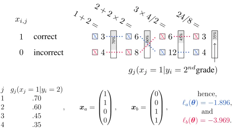
Figure 2.2 shows an example comparing `i values for two different response
patterns with given g(x|yi;θ) values for each item while both have same latent
variable levelyi = ‘2ndgrade0. In this context yi can be referred to as ability. We can
see that intuitively and numerically the response pattern xb is less plausible given
the model parameters. In this example, individual b answered questions that are ordered according to their difficulty level, such that the most difficult questions were answered correctly and, yet the easier questions answered incorrectly.
However, there are two caveats to this procedure: First, `i(θ) is not standardised.
x
i,j1
0
correct
incorrect
4
3
70%1 +
2 =
8
6
60%2 +
2
×
2 =
12
6
45%3
×
4
/
2 =
4
3
35%24
/
8 =
g
j(
x
j= 1
|
y
i= 2
ndgrade)
X
X
X
X
X
X
X
X
Please calculate the solution.
j gj(xj = 1|yi = 2)
1 .70
2 .60
3 .45
4 .35
, xa = 1 1 0 0
, xb = 0 0 1 1 , hence,
`a(θ) =−1.896,
and
[image:44.595.136.518.126.339.2]`b(θ) = −3.969.
Figure 2.2: Illustrative example of the individual log-likelihood contribution `i(θ),
for two response patterns labelled a and b.
unknown, it is difficult to actually classify a response pattern as model aberrant. Therefore, Drasgow et al. (1985) proposed a standardised version of `i(θ):
`∗i(θ) =
`i(θ)−E(`i(θ))
[Var(`i(θ))]1/2
(2.15)
where the expectation of `i(θ) is defined as
E(`i(θ)) = p X
j=1
{gj(xj = 1|yi;θj) ln[gj(xj = 1|yi;θj)]+
[1−gj(xj = 1|yi;θj)] ln[1−gj(xj = 1|yi;θj)]}
(2.16)
and the variance of `i(θ) can be written as
Var(`i(θ)) = p X
j=1
gj(xj = 1|yi;θj)[1−gj(xj = 1|yi;θj)][ln
gj(xj = 1|yi;θj)
1−gj(xj = 1|yi;θj)
]2.
The theoretical distribution of `∗
i(θ) under the true values of yi is supposed to be
standard normally distributed (Molenaar and Hoijtink, 1990, 1996). However, as was said before, any replacement of true parameter values by their respective maximum likelihood estimator generally has an impact on the distribution of person-fit statistics (Molenaar and Hoijtink, 1990; Nering, 1995, 1997; Reise, 1995). In this case, the variance of`i(θ) usually is smaller than expected. Even attempts to correct a smaller
empirical Type I error in contrast to the nominal one (e.g, using Warm’syi estimator)
could not account for overestimated positive and underestimated negative values of yi (van Krimpen-Stoop and Meijer, 1999).
Ordered categorical Models
There are existing generalisations of binary-logistic model person-fit indices which are feasible for measuring a participant’s misfit to ordinal categorical responses. The most commonly used model for such items is the ordinal logistic model (known in IRT literature as Graded Response Model, GRM; Samejima, 1970). Suppose there are U response categoriesu= 1, . . . , U. In the GRM we model the probability of responding to an observed variable giveny in or above a category u, i.e. gj(xj ≥u|y;αj, γj,u) as
gj(xj ≥u|y;αj, γj,u) =
exp[αj(y−γj,u)]
1 + exp[αj(y−γj,u)]
, (2.18)
for u = 2, . . . , U and gj(xj ≥ 1|y;αj, γj,u) = 1, thereby extending αj to a slope
parameter and γj,u to a threshold parameter. Here the item parameters are θj =
(αj, γj,2, . . . , γj,U). The joint distribution of the items given y is then given by
g(x|y;θ) =
p Y
j=1
Pr(Xj =xj|y;θj), (2.19)
where the probabilities Pr(Xj =xj|y;θj) are derived from (2.18).
In a model with ordered categorical responses we can use a generalisation of (2.14), the individual log-likelihood contribution
`grmi (θ) = p X
j=1
X
u