2016 International Conference on Computer, Mechatronics and Electronic Engineering (CMEE 2016) ISBN: 978-1-60595-406-6
A Mid-Term Voltage Stability Stochastic Analysis Method
Shi-ping XIAN and Yu-long HUANG
Institute of Electrical Automation, Jinan University, Zhuhai, Guangdong Province, China
Keywords: Mid and long-term voltage stability, Latin hypercube sampling, Trajectory sensitivity.
Abstract. This paper introduced the detail steps of Latin hypercube sampling method in mid-term voltage stability analysis considering uncertainty of load and wind generation power. Then by introduction of quasi steady trajectory sensitivity, the corresponding sampling efficient is highly improved. Finally it is demonstrated on IEEE 14 bus system that it’s feasible to use the quasi steady trajectory sensitivity to solve the problems of mid-term voltage stability associated with randomness
and it’s more efficient than the time domain simulation.
Introduction
With the increasing penetration of wind power and solar power in power system, many researchers [1-7] have studied voltage stability considering the uncertainties like wind power and load fluctuations. Ref. [1] discussed the relationship among the characteristics including volatility, intermittent and randomness of wind power. Ref. [2] demonstrated that stability of grid voltage will descend when attaching a wind farm, such as decline of stability margin, drops of terminal voltage and so on. Ref. [3,4] studied the impact of different kinds of wind turbine under different control modes on system voltage. Ref. [5] discussed the positive accumulation of small fluctuations will lead to a sudden instability of the system voltage, but it is only considering the effect of reactive load fluctuations in the system voltage stability, without taking the fluctuations of active load into account.
Ref.[6] analyzed and demonstrated that Speed Railway will do harm to power quality by bringing the
harmonics and negative sequence current into the power system as a power load with characteristic of frequent fluctuations and impact resistance. Ref. [7] used the theoretical prediction interval to solve problem of active power system optimal power flow in order to analyze the randomness and volatility of wind power output and load.
This article will consider the uncertainty of active power of wind turbine and load to perform stochastic simulation of mid-term voltage stability. Firstly use Latin Hypercube Sampling (LHS) to sample the initial conditions of random variables. However traditional simple random sampling based on the Monte Carlo simulation method can get a high precision when the sample size is sufficiently large, but its drawback is time-consuming, especially when simulating large power system. While
trajectory sensitivity based on quasi-steady state model [8-11] has been widely used in the study of
influence of random variables small changes on the system voltage stability [12-15], it can speed up the
simulation speed through calculating the voltage variation under different sample conditions directly. And then the voltage deviations caused by various random samples are directly calculated with the use of quasi-steady trajectory sensitivities. Finally the randomness of system voltage stability is analyzed.
Latin Hypercube Sampling
LHS algorithm mainly focused on the relevant issues of control is usually used to getting the sample which has a same relevant with the input random variables through sorting the input sample matrices, commonly used method includes random sort [16], Cholesky decomposition [17], orthogonalization
method based on the sequence of Gram-Schmidt [18]and so on.
The number of variables is K, and the number of samples is N, LHS algorithm will divide each
sample from each cell, so you can ensure sampling for each random variable Xi can cover the entire probability space.
Studies have shown that the active power of load subject to normal distribution with mean μ of its
rated active load, and standard deviation i of 5% of its rated active load[19]. Since the expectation μ of
normal distribution is only positional parameters, so the shape of the function does not affect by the pan of its probability density function, so the fluctuations of load can be considered to subject to a
normal distribution with expected value μ of 0 and variance of 2i. Similarly, the volatility of active
power of wind turbine can be seen as a normal distribution. Detailed steps of LHS considering correlation are as follow:
1) Get the correlation coefficient matrix CX of the input random variables;
2) Calculate ρZij according to the equation ρZij= T(ρXij)·ρXij, where ρXij is the correlation
between the i-th row CX i and the j-th row CX j of the matrix CX , the conversion factor of normal
distribution T (ρXij) = 1 [21], then ρZij=ρXij, and obtain CZ=CX;
3) Calculate the lower triangular matrix B through doing Cholesky decomposition on CZ;
4) Randomly sample K independent random variables subjected to stander normal distribution
(mean of 0, variance of 1), and form a matrix WK·N;
5) Calculate the matrix ZK·N with the equation Z=B·W, andthen get its order matrix LZ;
6) Take samples subjected to uniform distribution from Interval [0,1] to form a matrix UK·N;
7) Get the matrix Y whose elements Yijcan be calculate by the equation:
Yij=(j+ Uij-1)/N; (1)
8) Calculate the initial sample matrix XK·N = Φ-1(Y), where Φ is the standard normal cumulative
distribution function;
9) X will be reordered basing on the order matrix LZ to obtain a final sample matrix SK·N;
where K random variables required in the step (4) must be independent, which means that the correlation coefficient matrix is the identity matrix. According to Ref. [22], we can get independent random variables through processing the normal matrix by Gram-Schmidt sequence orthogonal algorithm:
1) Generate a random matrix EK·N subjected to standard normal distribution, then get its order
matrix RK·N as the initial matrix of Gram-Schmidt sequence orthogonal method;
2) Calculate correlation matrix ρK·N of matrix R and then calculate the root mean square
correlation ρ2rmsof matrix ρ with equation
1 2
2 1
2
0.5 1
j K
ij
j i
rms R
N N
; (2)
3) Take the forward step of the ranked Gram-Schmidt (RGS):
2 :1: 1
,
i i j
i i
for j K
for i j
R takeout R R
R rank R
,
where the function takeout (Ri, Rj) is to denote the residuals from a linear regression (including an
intercept) of the vector Ri on the vector Rj, the function rank (Ri) denotes the vector of ranks of Ri;
4) Then take the backward step of RGS:
1:1: 1
,
i i j
i i
for j K
for i K j
R takeout R R
R rank R
5) Through repeated iteration of forward and backward, the correlation ratio of the order matrix
R obtained after each iteration is smaller than the previous, the calculation end with the mark that the
value of ρ2rms is no longer reduced, then we can get the final order matrix R with lowest correlation;
6) Finally, get the matrix WK·N subjected to standard normal distribution by reordering the initial
sample matrix E with the order of matrix R, then each variables of WK·N can be considered as
independent.
Quasi Steady Trajectory Sensitivity [23, 25]
Under the quasi-steady state assumption, when a coupled system decomposes on the time scale, then its short-term dynamic process can be instead by its equilibrium equation and then obtained the model of quasi-steady state simulation as follow:
0 , , , ,
0 , , , ,
, , , ,
1 , , , ,
c d
c d
c c c d
d d c d
f x y z z
g x y z z
z h x y z z
z k h x y z z k
. (3)
where x is a column vector of time-varying transient variable associated with the generator rotor,
AVR, excitation system and induction motor; y is a column vector of varying algebraic variables
constructed by bus voltage magnitude and phase angle; zc is a column vector of time-varying
continuous state variable associated with internal dynamic process of automatic recovery load and
secondary voltage control; zd is a column vector of time-varying discrete state variable consist of
generator over excitation restrictions and limitations of the stator over current ; λ is a column vector
constituted by a variety of different control variables, such as can switching capacitor banks reactive power, load tap change ratio, the pilot bus voltage settings.
VSCF Doubly-fed Wind Generator [24, 26]
Doubly-fed induction generator (DFIG) are widely used in power system attached with wind power because of its characteristics that providing constant output frequency under different speeds.
Main equations of DFIG are as follow: 1) Rotor rotation equation
2
m e
m
m
T T
H
. (4)
where ωm is rotor angular speed, Tm is mechanical torque, Te is the electromagnetic torque, Hm is rotor
inertia.
2) Pitch angle control equation
P m ref P
p
P
K
T
. (5)
where θP is the pitch angle, KP is amplification factor of the pitch control, TP is time constant in the
pitch control, ωref is reference angular velocity.
3) Power regulation equation
*1 s m 1
qr qr
m
x x p
i i
T x V
4) Voltage regulator equation
dr v ref V dr
i K V V i
x
. (7)
where iqr, idr are current component of q, d-axis in the rotor coil, V is the terminal voltage, Vref is
reference voltage, xs is stator inductance, xμ is mutual inductance, Tε is time constant in power control,
Kv is amplification factor of the voltage control, p*ω(ωm) is the power-speed characteristic which
roughly optimizes the wind energy capture and is calculated using the current rotor speed value, as follows:
*0 0.5
2 1 0.5 1
1 1
m
m m m
m
P
. (8)
Random variable of wind turbine is the initial value of active power inject to the bus Pw0 and it
obeys the normal distribution Pw0~N(Pw0, (0.05Pw0)2).
Exponential Recovery Load [26]
Considering Load self-healing features, the dynamic characteristics of load can be described by the addition automatic recovery model:
0 0
0 0
s t
p
p L L
p
x V V
x P P
T V V
, (9)
0 0
0 0
s t
q
q L L
q
x V V
x Q Q
T V V
. (10) The power consumed by load can be described as:
0 0
t
p
L L
p
x V
P P
T V
, (11)
0 0
t
q
L L
q
x V
Q Q
T V
. (12)
where xp, xq are the dimensionless state variables relevant to the dynamic characteristics of the load,
Tp, Tq are the recovery time constant of active and reactive power load, αs, αt, βs, βt are characteristic
index of static and transient voltage, PL0, QL0, V0 are the load active power, reactive power, bus
voltage in steady-state operation.
The random variables of load are its initial value of power PL0 and QL0 which are subjected to
distribution PL0~N(PL0, (0.05PL0)2), QL0~N(QL0, (0.05QL0)2).
Finally we can obtain the distribution of the variation of PL0, QL0, Pw0, as following:
PL0~N(0, (0.05PL0)2), QL0~N(0, (0.05QL0)2), Pw0~N(0, (0.05Pw0)2).
Trajectory Sensitivity Analysis [25]
Firstly calculate trajectory sensitivity of bus voltages to random variables based on the voltages
trajectory V0 of deterministic simulation S=
0 0 0
i i i
L L w
V V V
P Q P
Then calculate the corresponding voltage variation V=[V1,...,Vn] T directly according to the
sampling results X=[PL0QL0Pw0] T of LHS with the equation V=S·X.
Finally add the voltage variation to the original track and then get voltage trajectory curve
V=V0+V under different samples.
Simulation Result
Power system analysis tool (Psat) [26] is used to simulate IEEE14 bus system, with computer
memory 4G, CPU clocked at 2.4Hz.
Synchronous generators are 6-order model, and taking the impact IEEE DC type-2 exciter into account, load is described by exponential recovery type load model. Simulation time is set as 100s, the simulation step is 2s.
Number of load in system is 11, and their numbers are 2, 3, 4, 5, 6, 9, 10, 11, 12, 13 and 14. The
correlation matrix Cx similar to Ref. [21] describes the correlation of different load.
1 0.5 0.8 0.7 0.6 0 0 0 0 0 0
0.5 1 0.7 0.6 0.8 0 0 0 0 0 0
0.8 0.7 1 0.5 0.6 0 0 0 0 0 0
0.7 0.6 0.5 1 0.9 0 0 0 0 0 0
0.6 0.8 0.6 0.9 1 0 0 0 0 0 0
0 0 0 0 0 1 0.5 0.8 0.7 0.6 0.4
0 0 0 0 0 0.5 1 0.7 0.6 0.8 0.5
0 0 0 0 0 0.8 0.7 1 0.5 0.6 0.5
0 0 0 0 0 0.7 0.6 0.5 1 0.9 0.6
0 0 0 0 0 0.6 0.8 0.6 0.9 1
X
C
0.6
0 0 0 0 0 0.4 0.5 0.5 0.6 0.6 1
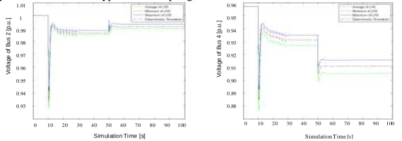
Bus 2 is connected with DFIG units, and the other four buses (1, 3, 6 and 8) are connected with synchronous generator units.
Disturbance is set as ascending gradually of the load from 10s to 30s (increasing from the initial value to 110% of the initial value), and then disconnection fault between Bus 2 and Bus 4 occurs in 50s.)
In this paper, sample size N set as 100, using LHS to sample, then carry out time domain
simulation, and recording terminal voltage of wind turbine and the total time of domain simulation ttd.
Analysis results of Latin Hypercube Sampling
Simulation Time [s] 1.01
1
0.99
0.98
0.97
0.96
0.95
0.94
0.93
20 30 40 50 60 70 80 90
0 10 100
V
o
lt
a
g
e
o
f
B
u
s
2
[
p
.u
.]
Simulation T ime [s]
0.96
0.95
0.94
0.93
0.92
0.91
0.90
0.89
0.88
20 30 40 50 60 70 80 90
0 10 100
V
o
lt
a
g
e
o
f
B
u
s
4
[
p
.u
[image:5.595.93.503.496.640.2].]
Figure 1. Comparison of random sampling and deterministic simulation.
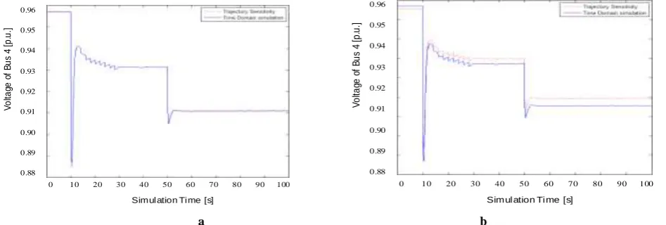
Comparison of Trajectory Sensitivity and Time-domain Simulation
Calculate trajectory sensitivity matrix S of the deterministic simulation, then calculate the voltage
variation Vwith the sampling results X of LHS, and finally obtain bus voltages V.
Figure 2 compared the voltage curve of load bus obtained from trajectory sensitivity calculations and time-domain simulation in different samples.
Simulation Time [s]
0.96 0.95 0.94 0.93 0.92 0.91 0.90 0.89 0.88
20 30 40 50 60 70 80 90 0 10 100
V
o
lta
ge
o
f
B
u
s
4
[p
.u
.]
Simul ation Ti me [s]
0.96 0.95 0.94 0.93 0.92 0.91 0.90 0.89 0.88
20 30 40 50 60 70 80 90
0 10 100
V
o
lta
ge
o
f
B
u
s
4
[p
.u
.]
[image:6.595.63.537.151.311.2]a b
Figure 2. Voltage curves of Trajectory sensitivity and Time-domain simulation in Bus 4.
[image:6.595.160.436.401.596.2]Figure 2 (a) responses the result with a relatively small error between trajectory sensitivity and time domain simulation, it can be seen that the two curves are almost coincident; while the error shown in Figure 2 (b) is bigger. We can see the detailed errors of voltage in each bus in the table as follow:
Table 1. Relative error of Trajectory sensitivity and Time-domain simulation.
Bus
Maximum of error [%] Num
Simulatio n times [s]
Minimum of error
[10e-4%] Num
Simulation time [s]
Average error [%]
1 0.6709 9 10.125 0.0175 79 80.625 0.0413
2 0.7153 9 10.125 -0.027 84 56.375 0.0542
3 0.5853 9 10.25 0.0006 51 52.125 0.0264
4 0.7757 4 10.25 0.0103 31 35.75 0.1010
5 0.7253 4 10.25 -0.015 55 13.75 0.0839
6 -0.8075 58 6.375 0.0154 38 81.625 0.0763
7 0.9384 4 10.25 0.0185 95 73 0.1104
8 0.7991 4 10.25 -0.007 64 98.875 0.0530
9 1.0855 4 10.25 -0.039 55 11.125 0.1511
10 1.0315 4 10.25 -0.412 2 28.625 0.1458
11 -0.9056 58 6.375 -0.011 25 51.25 0.1053
12 0.9717 54 10.25 -0.094 30 83.75 0.1085
13 0.9688 54 10.25 -0.037 18 45.5 0.1195
14 1.1940 54 10.25 -0.607 89 18.125 0.1601
The relative error between trajectory sensitivity and time domain simulation is shown in Table 1. It can be seen that the biggest error occurs in Bus 14 at 10.25s, and reach 1.19%, while the smallest error is almost negligible. In addition, the average error of each bus is guaranteed at less than 0.2%.
Table 2 shows simulation time of the Trajectory sensitivity and Time-domain simulation methods. The time of trajectory sensitivity simulation is much less and more efficient.
Table 2. Simulation time of Trajectory sensitivity and Time-domain simulation.
Simulation method Time-domain simulation ttd Trajectory sensitivity tts
Simulation time [s] 4 225.700 22.526
Summary
This article describes the detail steps of Latin Hypercube Sampling algorithm considering correlation of random variables, and demonstrates that it’s feasible and efficient to use the quasi-steady trajectory sensitivity in mid-term voltage stability analysis associated with uncertainty like load and wind power.
Acknowledgement
This work was financially supported by Collaborative Innovation Center in Zhuhai.
References
[1]Xue Yusheng, A Review on Impacts of Wind Power Uncertainties on Power Systems [J].
Proceedings of the CSEE, 2014, 34(29):5029-5040.
[2] Zou Zhixiang, Analysis on Influences of Grid-Connected Wind Farm on Voltage Stability of
Local Power Network Neighboring to Connection Point [J]. Power System Technology, 2011, 35(11): 50-56.
[3]R. R. Londero, C. M. Affonso, J. P. A. Vieira, Impact of Different DFIG Wind Turbines Control
Modes on Long-Term Voltage Stability [J]. IEEE PES Innovative Smart Grid Technologies Europe (ISGT Europe), 2012. 1-7.
[4]Rafael Rorato Londero, Carolina de Mattos Affonso, João Paulo Abreu Vieira, Long-Term
Voltage Stability Analysis of Variable Speed Wind Generators [J]. IEEE Transactions On Power Systems, 2015, 30(1): 439-447.
[5]Qiu Yan, Effect of Stochastic Load Disturbance on Power System Voltage Stability [J]. Electric
Power Automation Equipment, 2009, 29(2):77-81.
[6]Liu Yuquan, Wu Guopei, Effect of High-speed Railway Traction Load on Power System
[J].Power System Protection and Control, 2011, 39(18): 150-154.
[7]Lin Haiming, Optimal Active Power Flow Considering Uncertainties of Wind Power Output and
Load [J] Power System Technology, 2013, 37(6): 1584-1589
[8]Cutsem T.V., Vournas C.D., Voltage stability analysis in transient and mid-term time scales [J].
IEEE Trans. on Power Systems, 1996, 11(1): 146-154.
[9]Cutsem T.V., Jacquemart Y., Marquet J.N., et al. A Comprehensive Analysis of Mid-term
Voltage Stability[J]. IEEE Trans. on Power System, 1995, 10(3): 1173-1182.
[10]Cutsem T.V., An Approach to Corrective Control of Voltage Instability Using Simulation and
Sensitivity[J]. IEEE Trans. on Power Systems, 1995, 10(2): 616-622.
[11]Cutsem T.V., Mailhot R., Validation of a Fast Voltage Stability Analysis Method on the
Hydro-Quebec System[J]. IEEE Trans. on Power Systems, 1997, 12(1): 282-292.
[12]Dan Suriyamongkol, Hany A. Abdelsalam, Elham B.Makram, Trajectory Sensitivity Analysis
Application for Power System Security Assessment with Wind Generation [J]. North American Power Symposium (NAPS), 2015: 1-6.
[13]Amin Nasri, Mehrdad Ghandhari, Robert Eriksson. Transient Stability Assessment of Power
Systems in the Presence of Shunt Compensators Using Trajectory Sensitivity Analysis [J].IEEE Power & Energy Society General Meeting, 2013: 1-5.
[14]Huang Yilong, Model Predict Control of Long-term Voltage Stability Based on Corrective
[15]Hu Yangyu, A Method to Analyze Trajectory Sensitivity of Voltage Stability Based on Quasi-Steady State Simulation [J]. Power System Technology, 2012, 36(6): 157-162.
[16]McKay M D, Beckman R J, Conover W J, A Comparison of Three Methods for Selecting Values
of Input Variables in the Analysis of Output From a Computer Code[J]. Technometrics, 1979, 21(2): 239-245.
[17]Iman R L, Conover W J, A Distribution-free Approach to Inducing Rank Correlation Among
Input Variables [J]. Communications in Statistics-Simulation and Computation, 1982, 11(3):311-334.
[18]Owen A, Controlling Correlations in Latin Hypercube Samples [J]. Journal of the American
Statistical Association, 1994, 89(428): 1517-1522.
[19]Ding Ming, Probabilistic Load Flow Evaluation with Extended Latin Hypercube Sampling [J].
Proceedings of the CSEE, 2013, 34(4): 163-170.
[20]Luo Gang, Fast Calculation of Probabilistic Available Transfer Capability Considering
Correlation in Wind Power Integrated Systems [J]. Proceedings of the CSEE, 2014, 34(7): 1024-1032.
[21]Chen Yan, Probabilistic Load Flow Analysis Considering Dependencies Among Input Random
Variables [J]. Proceedings of the CSEE, 2011, 31(22): 80-87.
[22]Art B. Owen, Controlling Correlations in Latin Hypercube Samples [J]. Journal of the American
Statistical Association, 1994, 89(428): 1517-1522.
[23]Hu Bo, Research on Novel Methodologies of Coordinated Voltage Control in Electric Power
Systems [D]. South China University of Technology, 2010.
[24]Liu Yanzhang, Medium and Long-Term Time Scale Modeling for Variable Speed Constant
Frequency Wind Turbines [J]. Power System and Clean Energy, 2014, 30(10): 111-118.
[25]Huang Yulong, A Dissertation Submitted for the Degree of Doctor of Philosophy in Electrical
Engineering [D]. South China University of Technology, 2012.
[26]Milano F. Documentation for PSAT version 2.0.0. [ED/OL].