1030
A SYSTEM FOR RAPID LOCALIZATION AND INTENSITY
EVALUATION OF SAPONINS ACCUMULATION IN PLANT
TISSUES
1MELA G. ABDUL-HALEEM, 2Dr. LOAY E. GEORGE, 3Dr. ANSAM G. ABDUL-HALEEM
1,2Department of Computer Science, University of Baghdad, Iraq
3Department of Biology Science, University of Baghdad, Iraq
E-mail: 1[email protected], 2[email protected], 3[email protected]
ABSTRACT
A fluorescence microscopy considered as a powerful imaging tool in biology and medicine. In addition to useful signal obtained from fluorescence microscopy, there are some defects in its images such as random variation in brightness, noise that caused by photon detection and some background pixels in the acquired fluorescence microscopic images appear wrongly auto-fluorescence property. All these practical limitations have a negative impact on the correct vision and analysis of the fluorescent microscope users. Our research enters the field of automation of image processing and image analysis using image processing techniques
and applying this processing and analysis on one of the very important experiments in biology science.
This research is devoted to develop a system based on digital image processing methodology to localize and assess the concentration of saponins accumulation in plant tissues using Fluorescence microscopic image. The proposed system involved preprocessing steps than to make the region of interest more obvious and reflects the saponins accumulation area. Also, the system introduces a simple mathematical way for concentration assessment, and it was justified through the test results. It includes building a system to get microscopic images with best appearance and no defects. It determines the saponins accumulation sites in
leaves, rhizomes and shoot apex of Y. gloriosa Variegata and their in vitro cultured tissues (Calli, direct and
indirect regenerated shoots and rhizomes/roots). Statistical analysis is performed using a computer to get the mean and median of saponins intensities in each part, and finally perform a comparison between them to determine which part can record the highest intensity level of saponins. The results showed high ability of the system to determine the locations and intensity of saponins in the different parts of the plant. It
performs the statistical analysis very quickly. In in vitro culture, it was found that callus treated with
Thidiazuron (TDZ) in a combination with benzyl aminopurine (BA) and naphthyl acetic acid (NAA) after 3 weeks of culture had the highest level of saponins accumulation, while the leaves of intact plant recorded the second highest accumulation of saponins.
Keywords: Fluorescence Microscopy, Histogram Statistics, Contrast Stretching, region of interest (ROI), Saponins intensity
1. INTRODUCTION
Microscopy imaging includes fluorescence microscopy and electron microscopy, has taken a prominent role in life science research and medicine due to its ability to investigate the 3D interior of live cells and organisms [1]. One essential advantage of fluorescence microscopy is the presence of fluorescent molecules themselves
(Auto-fluorescence). Auto-fluorescence is a
phenomenon that consists of the emission of light in the visible spectral range of ultraviolet radiation,
when biological substrates affected by light at an appropriate wavelength. On the other hand, specific fluorochromes can be added to the specimen, depending on what is being investigated [2].
To obtain a fluorescent image from fluorescence microscopy, there are four basic processes which include fluorophore excitation,
Photon emission, Photon detection and
quantification and storage. After the specimen has been prepared and is putting underneath the
1031 (fluorophores) must be converted into an excited state by absorption of a photon. This is done by illuminating the specimen, with a lamp or laser. Then each fluorophore may emit a photon with a lower energy (i.e. longer wavelength) than the photon previously absorbed. A part of the light should enter the objective lens of the microscope and be focused towards a detector. When a photon hits the detector, it releases an electron. After a fixed time interval, the charges of a set of such electrons are quantified, and pixel values are determined from these quantified. A larger charge is translated into a higher pixel value [3].
Although, the big advantages of using fluorescent microscope in biological domain, but like all techniques, it is subject to practical limitations. The recent developments with fluorescent microscopy concern with improvement of image quality by addressing the basic problem of image resolution. It is determined by image contrast (i.e., Uncertainty in brightness), the diffraction of light within optical systems that results in blurring the image and the noise that can be formed from imprecisions when the charge of small clouds of electrons are determined quickly. In fact, the emission of the photons is itself random, so we would still get noisy images even if we detected every photon perfectly [3, 4]. To overcome on all of these limitations the image processing techniques are used. As well as, Image processing techniques provides more advantages than traditional methods of analysis: 1) In spite of the human vision is very sensitive, but it can be easily biased from preconceived notions of objects and concepts; while automated image analysis provides an unbiased approach to extract information from image data and test assumptions. 2) Once a routine has been developed for image analysis, it can be applied to a large number of microscopic images, so, image processing techniques facilitate the collection of large amounts of data for statistical analysis.
In this research, many image processing routines are used to overcome on the limitations of fluorescence microscopy. A simple and fast method for saponins regions is introduced. The developed algorithm offers a comprehensive scenario can
handle automatically detect the saponins
accumulation regions and assess its concentration. Saponins are the most important components of medicinally important plants. The accumulation of these compounds in leaves, rhizomes and shoot
apex of Y. gloriosa Variegata and their in vitro
cultured tissues (calli, direct and indirect regenerated shoots and rhizomes/roots) is
performed by calculating the mean and median of intensity values of saponins in these parts.
Steriodal saponins are important active
components of Yucca gloriosa Variegata, a
medicinally important plant. However, most studies on Y. gloriosa have mainly focused on the
components analysis, pharmacology and medicinal treatments. Saponins are glycosylated natural products, a vast group of structurally diverse glycosides of the plant kingdom and also of some marine organisms and insects [5]. They have a high molecular weight. They are able to interact with cell membranes and are able to decrease the surface tension of an aqueous solution [6], and these surface active properties distinguished them from other glycosides, beneficiary from them in industrial applications as foaming and surface active agents. They contain a steroidal or triterpenoid aglycone and one or more sugar chains. The detection and localization of saponins accumulation are very necessary to determine which plant organ or tissue accumulates high levels of such important compounds.
Some of related works are shown in the next section. A brief description for basic tasks involved in the proposed system is introduced in section 3. The results of the image enhancement and isolation of saponins sites, and the mean and median values
for saponins intensity are explained in
the experimental data and results section. Finally, the main conclusions derived in this work and a list of recommendations for future works are presented in the conclusion section.
2. RELATED WORK
Some of the published works related to image processing and fluorescence microscopy techniques are given in the following paragraphs:
Du and Dua [7], used k-means clustering, EM, Otsu’s threshold, and GMAC methods for unsupervised learning in cell image segmentation. A comparison were performed between these methods are compared to show strengths of efficiency and embedded limitations.
Matula [8] concerned with digital image processing in fluorescence microscopy and its use in cell biological experiments. The work was conceived as a collection of 26 scientific articles divided into four groups according to areas that they contribute to (1) automation of image acqusition and image analysis, (2) image segmentation, (3) object tracking and (4) applications in the cell nucleus research.
1032
Kervrann et al. [1] introduced advances in
fluorescence and electron microscopy and determined the image processing and analysis methods required to quantify phenotypes for a limited number but typical studies in cell imaging.
Chang et al. [9], analyzed proliferation,
kinematics and attachment of mouse embryonic stem cells using time-series confocal time-lapse fluorescence microscopy images by using an automated image processing technique. The results of the implementation showed that the automatic method can successfully analyze cell kinetics, proliferation and attachment.
3. SYSTEM LAYOUT
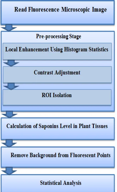
[image:3.612.96.298.355.687.2]The proposed system has the essential stages to perform all relevant pre-processing, segmentation (i.e., ROI isolation) and statistical analysis tasks. The general structure of the proposed model is shown in Figure (1).
Figure 1: The proposed model architecture.
As clarified in Figure 1, the system consists of three stages (i) preprocessing, (ii) allocation the saponins region & (iii) statistical analysis for estimating the level strength of saponins accumulation. All introduced methods a simple and fast, it can be used to accomplish the whole accumulation and assessment task automatically without need for conducting algorithms have high-complicated cost.
2.1 Read Fluorescence Microscopic Images The fluorescence microscopic image is fed to the system as a Bitmap (BMP) image file; the color resolution of the image is taken 24 bits per pixel (bpp). The image data (i.e. Red, Green, Blue (RGB) components) is loaded.
2.2 Pre-processing Stage
The main focus of this stage is to enhance the image for subsequent pattern recognition and to overcome on the drawbacks of fluorescence microscopy. This phase includes many steps: 2.2.1Local enhancement using histogram
statistics
The histogram statistics are used to enhance details over small areas in an image. For each different intensity value, the histogram represents the number of pixels in an image which have this value. The histogram for 8-bit gray image will graphically display 256 numbers for 256 different possible intensities gray scale values. Histograms can also be taken of color images either by taking the individual histogram of red, green and blue channels, or a three dimensions (3-D) histogram can be produced, with the three axes representing the red, blue and green channels can be taken. The operation includes scanning the image in a single pass and counting the number of pixels found at each intensity value. This is used to construct a suitable histogram [10, 11].
2.2.2 Contrast adjustment
1033 obtained just by taking the minimum and maximum pixel values that the image type concerned [12]. In this research, the upper and lower pixel value limits are obtained by using the histogram and thresholding technique for blue color.
A. Gamma Stretching
One of the best intensity transformations that will improve the appearance of the images is gamma contrast adjustment. When preparing imagery for computer display; gamma is the degree of contrast between the mid-level gray values of an image and it does not have any effect on the black or white values of an image. By applying a gamma correction, the overall brightness of an image can be improved. If the gamma value is set too high, middle tones appear too dark; however, if the gamma value is set too low, middle tones appear too light and the image looks bleached out. Additionally, Gamma can change the ratios of red to green to blue [13]. A target color can be determined so the gamma is calculated based on the present average color of the raster and user-specified target color. Algorithm (1) shows the main steps to perform this process. For calculation of best threshold used in calculation of minimum gray level, the value of α is set to (0.002) while for maximum gray level and it is set to (0.01). Also, the inclusion parameter (E1) in gamma stretching equation for blue color is set to 3.5, and the inclusion parameter (E2) is set to 5.
Algorithm (1) : Histogram Calculation and
Gamma Stretching
Goal: intensity transformation
Input: RGB components
Output: new-blue(), new-Green(), new-Red()
Step 1: Calculate Histogram for blue color of RGB image.
For all pixels of image
his(i) ←his(Blue(x,y)) + 1 End For
Step 2: Calculate the minimum and maximum pixel values that the image type concerned.
Step 2.1: Calculate minimum value and select a threshold as a small ratio of the image area.
Thr ← α * (W id * Hgt) For all i=0→255 sum ←
check If sum <= Thr Then Min ← i
Exit Loop
End if End For
Step 2.2: Calculate maximum value and select a threshold as a small ratio of area of the image.
Thr ← α * (Wid * Hgt) For all i=255→i
sum ←
check If sum >= Thr Then Max ← i: Exit Loop : End if
End For
Step 3: Do Gamma filter Stretching for Blue and Green colors.
For all i → Min + 1 To Max - 1
Table-B(i) ←
Table-G(i) ←
End For
Step4: Get the new RGB components. New-Blue(x, y) ← Blue(x, y) + 2 * Table-B (Blue (x, y)) / 3
New-Green(x, y) ← Table-G( Blue (x, y)) New-Red(x, y) ← 0
Step5: Return Blue(), Green(), New-Red().
B. Linear Stretching
Histogram of an image is analyzed based upon brightness and contrast of the image. If the histogram of the image is dark, the pixels of the image move towards the lower gray level region. If the histogram of the image is bright, the pixels of the image move towards the higher gray level region. The histogram will not be equally spread if it is a low contrast image. The histogram will be equally spread if it is of high contrast. Linear stretching and histogram equalization are the two methods of histogram manipulation. In linear stretching, the dynamic range of the image is increased while the shape of the histogram is not
altered [14]. This step is used to increase the
dynamic range of blue color. The process starts with calculation the histogram of blue color of each pixel resulted from the previous step. The minimum and maximum level is obtained in the same way. Then, linear stretching equation (1) is applied. For calculation of best threshold used in calculation of minimum and maximum gray level, the value of α is set to (0.001) as shown in algorithm (2).
1034
Where is blue pixel, is the
transformation function of linear stretching, the original gray level are [min, max], and the target gray levels are [0, 255].
Algorithm (2) : linear Stretching
Goal: increase the dynamic range of blue color
Input: new-blue(), new-Green(), new-Red()
Output: final-blue(), final-Green(), final-Red()
Step 1: Calculate Histogram for new blue color of RGB image.
For all pixels of image //x width index, y for height index
his(i) ←his(new-Blue(x,y)) + 1 End For
Step 2: Calculate the minimum and maximum pixel values that the image type concerned.
Step 2.1: Calculate minimum value and select a threshold as a small ratio of the image area.
Thr ← α * (W id * Hgt) For all i=0→255 sum ←
check If sum <= Thr Then Min ← I
Exit Loop End if End For
Step 2.2: Calculate maximum value and select a threshold as a small ratio of area of the image.
Thr ← α * (W id * Hgt) For all i=255→i
sum ←
check If sum >= Thr Then Max ← i: Exit Loop : End if
End For
Step 3: Do linear filter Stretching for Blue and Green colors.
For all i → Min + 1 To Max - 1
Table-B (i) ← //
equation (1). End For
Step4: Get the new RGB components.
final-Blue(x, y) ← Table-B (new-Blue (x, y))
final-Green(x, y) ← new-Green (x, y) final-Red(x, y) ← new-Red (x, y)
Step5: Return final-Blue (), final-Green(), final-Red(x, y).
This step is used to increase the dynamic range of blue color. The process starts with calculation the histogram of blue color of each pixel resulted from the previous step. The minimum and maximum level is obtained in the same way. Then, linear stretching equation (1) is applied.
2.3 ROI Isolation
The ROI extraction is considered as a type of segmentation. After enhancement, the fluorescent region can be seen as a special island in the image. Using the seed filling principle with appropriate constrain lead to optimal segmentation of these regions by removal all other islands in the image. This method includes two steps: the first step is the identification of seeds. In case of island removal the seed point has foreground value. The second step includes constraints to prevent each region from overfilling. In this work, the selected constrain is that the selected filling region in case of segmentation must form very small ratio of the image area (0.3) otherwise it will be ignored. This process is shown in algorithm (3) and algorithm (4).
Algorithm(3):Seed Filling Function Goal: The number of pixels in seed region Inputs: p // target pixels
I // x-position of the target pixel J // y-position of the target pixel
Output: SS // the number of pixels in seed filling
region
Step 1 : Enter the pixel positions in an array Q Step 2 :Initialize pixel count to zero
Step 3 : While Q is not empty:
Step 4: Set n equal to the last element of Q. Step 5: Remove last element from Q. Step 6: Increase pixel count SS
Step 7 : Check If the color of n is equal to target-color:
Check If the west pixel value equal to the target value
Add west pixel to end of Q. End If
CheckIf the east pixel value equal to the target value
Add east pixel to end of Q. End If
CheckIf the north pixel value equal to the target value
1035 CheckIf the south pixel value equal to the target value
Add south pixel to end of Q. End If
End If End While
Step 8 : Return SS;
Algorithm(4): ROI isolation
Goal: fluorescent regions extraction Inputs: final-blue()
Output: seg() // island removal image
Step 1: Calculate Histogram for blue color of RGB image.
For all pixels of image //x width index, y for height index
his(i) ←his(final-Blue(x,y)) + 1 End For
Step 2: Calculate maximum value and select a threshold as a small ratio of area of the image.
Thr ← α * (W id * Hgt) // α = 0.02 For all i=255→i
sum ←
check If sum >= Thr Then Max ← i: Exit Loop : End if
End For Step 3: Select seed point
For all pixels of image
checkIf final-Blu(x, y) >= Max Then Tmp(x, y) = 1
End If End For
Step 4: Enter the constant criteria parameter C Step 5: Count the region ratio
rat← C × (Hgt × Wid) // C=0.3
Step 6: Search for each target pixel in all image and call seed function to each ones For all pixels in the Tmp image// x as row number, y as column number
CheckIf pixel value = 1 Then// seed pixel S ← seed (1, x_position, y_position);
//algorithm (3)
Step 7: Compare the number of pixels in the seed region with the region ratio
CheckIf S ≤ rat Then// keep region in the image
For all pixel in the image // i as row number, j as column number
CheckIf seed region(i,j) =1 Then
seg(i,j)←255 else seg(i,j)←0 End If
End For // i& j End If
End If
End For // x& y Step 8: Return seg();
2.4 Calculation of Saponins Level in Plant Tissues
The level of saponins in plant tissues can be determined by calculating the intensity of fluorescence in fluorescent sites which represent the sites of saponins accumulation in these tissues. This process includes obtaining gray image from the original color image. Then, only the gray-level of isolated sites are taken where the value of blue color after preprocessing equal to 255. The other pixel must be ignored (i.e., set to 0). The gray
image at position is determined as
the average of red, green, and blue bands as shown in equation (2) and algorithm (5).
(2)
Algorithm(5): Saponins level calculation
Goal: saponins intensity
Inputs: seg()
Output: fluorescent()
Step 1: Calculate gray image from the original RGB image.
For all pixels of image //x width index, y for height index
gray(x,y) ←Equation(2) End For
Step 2: Get the intensity for only fluorescent points
For all pixels of image //x width index, y for height index
checkIf seg (x,y) == 0 Then fluorescent (x,y) ←0 Else
fluorescent (x,y) ← gray(x,y) End if
End For
Step 3: Return fluorescent ();
1036 One of the defects of fluorescence microscopy is that the light starting from one point in the specimen cannot be focused back to a one point on the detector. Consequently, it can spread at the end over several pixels [3]. To get actual fluorescent points, the intensity value of each fluorescent pixel is subtracted from a local mean using equation (3). The local mean of each fluorescent pixel is calculated within (17×17) window that surrounding it.
(3)
Where represents the new intensity
value of pixel at position and
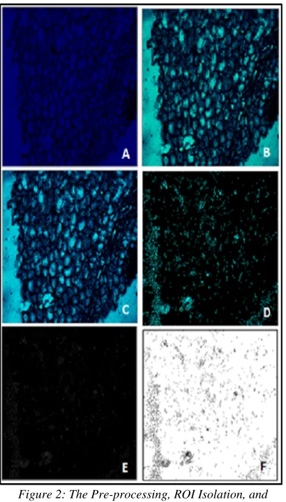
[image:7.612.92.297.305.665.2]represents its local mean. The applied previously mentioned steps are clarified in Figure (2).
Figure 2: The Pre-processing, ROI Isolation, and Intensity Calculation Processes;
A: An Image Acquired by a Fluorescence Microscopy; B: Gamma Stretching Effect; C: Linear Stretching Effect; D: ROI Isolation; E: Saponins Intensity Image with Black
Background; F: Saponins Intensity Image with White Background for Better View.
2.6 Statistical Analysis
The statistical analysis of input image is implemented using two measures like mean and median. The basic of all statistical measurements is mean. It is measured by calculating the average of all pixel values within m×n window. While median is the measure of intensity level of pixel. It works by selecting the middle pixel value from the ordered set of values within the ‘m×n’ window around the reference pixel. If the number of values in the set is an even number, then the average of the two values in the middle of the ordered set is taken [15]. Saponins accumulation is identified according to the fluorescent intensity. In this research, the mean and median of the intensity of fluorescent points only is calculated. To calculate mean and median, all fluorescent points are put in one dimension array and then the arithmetic formula of mean is performed as the following:
(4)
Where represents the number of fluorescent
points in the image and one dimension array
of all fluorescent points. To calculate median value,
the array is sorted in ascending order and
then the median value is taken as the following:
, (5)
3. EXPERIMENT AND RESULTS
A significant variation in the fluorescence and density between the classes of samples that represent anatomical sections of different parts of
the intact plant of Y. gloriosa Variegata (leaves,
rhizomes and shoot apex) and their in vitro cultured
tissues (Calli, direct and indirect regenerated shoots
and rhizomes/roots) were recorded. The
1037 The prior articles that contributed in the field of localization of saponins accumulation in Y. gloriosa Variegata plant are very little and they depended on using traditional methods of analysis or on the observed visualization in the fluorescent microscopic images by an expert or a biological researcher. While this research automatically detected on saponins accumulation and an automatic statistical analysis was performed where the decisions were made by a machine. So, only one article will be compared with this contribution. Abdul-Haleem [16] employed histological analysis and fluorescence microscopy techniques to determine the locations of saponins accumulation in
different parts of Y. gloriosa Variegata plant. Both
thin layer chromatography (TLC) analysis and High performance liquid chromatography (HPLC)
analysis of steroidal saponins from Y. gloriosa
Variegata extracts were used and matched the results with the observed visualization in the images of sections examined by fluorescence microscope. Abdul-Haleem [16] found that callus that treated with TDZ accumulated the highest amount of saponins. The results of this research were compatible with Abdul-Haleem [16] from which the samples were taken. These samples were acquired using UV light microscopy and by employing aniline blue stain to visualize saponins sites.
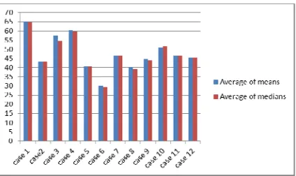
[image:8.612.91.303.574.700.2]The highest intensity of saponins was found in callus treated with TDZ in a combination with BA and NAA after 3 weeks where the average of means and medians of saponins intensity were 65.00 and 64.68, respectively. For intact plant, the highest accumulation of saponins was recorded in leaves which represented the second highest level of saponins accumulation. The average of saponins intensity means and medians in these leaves were 60.33 and 59.54, respectively as shown in Table (1) and Figure (4). Table (1) and Figure (3) are put at the end of the research.
Figure 4: Averages of Means and Medians at Each Class
4. CONCLUSIONS
In this research, we have presented an aid computerized system to localize saponins accumulation and evaluate the intensity of these
compounds in intact plant of Y. gloriosa Variegata
and their in vitro cultured tissues. The first part of
the system concerned with the treatment of the problems of fluorescence microscopy, which constituted a major obstacle for the biologists despite its great scientific importance. The use of image processing techniques is a key step to ensure that the right decision is taken by the biologist. Gamma and linear stretching are first carried out to adjust contrast in the acquired images. Our analysis shows that a correction is needed to highlight the fluorescent sites in low-light imaging. It is clear to observe that the proposed model gave good results for totally isolation of saponins accumulation sites. The desired result is highly affected by the correct selection of filling region. The region that forms the ratio (0.03%) of the image area gave the best possible result according to the selected dataset. The other part of the system concerned with performing a statistical analysis and applying this analysis on the biological experiment. The results showed the high ability of the system to determine intensity of saponins in the different parts of the plant and the highest level of saponins accumulation is found in callus treated with TDZ in a combination with BA and NAA after 3 weeks of culture. The variation in saponins accumulation was attributed to the type of growth regulators, initiation period, and plant part. These results and conclusions were compatible with the results obtained by a biology researcher. From those data, we were able to point out some strength in statistical significance.
This work can be extended to perform on other
important compounds in Y. gloriosa Variegata. In
addition, the system can be extended to include other/more statistical analysis. On the other hand, it can be also used in any biological experiments that require using fluorescence microscopy.
6. ACKNOWLEDGEMENTS
1038 REFRENCES
[1] C. Kervrann , C. O. Sorzano, S. T. Acton, J. Olivo- Marin, and Unser M, “A guided tour of selected image processing and analysis methods for fluorescence and electron microscopy,”
IEEE J Sel Top Signal Process, IEEE Signal Processing Society, Vol. 10, Issue 1, 2016 Feb,
pp. 6-30. Available from: hal-01246375 DOI: 10.1109/JSTSP.2015.2505402.
[2] A. C. Croce, and G. Bottiroli, “Autofluor-escence Spectroscopy and Imaging: A Tool for
Biomedical Research and Diagnosis,” Eur J
Histochem., Vol. 58, Issue 4, 2014 Oct 22, pp.
2461.Available from: DOI: 10.4081/ ejh.2014. 2461.
[3] P.Bankhead, Analyzing Fluorescence
Microsc-opy Images with Image J, UK: Queen's
university Belfast, 2014 May, 195p.
[4] M. J. Sanderson, I. Smith, I. Parker, M. D. Bootman, “Chapter1: Fluorescence Microsc-opy,” In: J. B. Parys, M. D. Bootman, D. I.
Yule, and G. Bultynck, editors, Calcium
Techniques: A Laboratory Manual, New York:
Cold Spring Harbor Laboratory Press, 2014,pp.
1-24.
[5] M. Thakur, M. F. Melzig, H. Fuchs, A. Weng, “Chemistry and pharmacology of saponins: special focus on cytotoxic properties. Botanics: Targets and Therapy, Vol. 1, 2011, pp. 19-29.
[6] P. M. Dewick, Medicinal Natural Products a
Biosynthetic Approach, 2nd ed. Wiley J, Sons.
Ltd, Electric ISBN: 0470846275, 2002, pp. 515. [7] X. Du, and S. Dua, “Segmentation of
fluorescence microscopy cell images using
unsupervised mining,” Open Med Inform J.,
Vol. 4, 2010 May 28, pp. 41–49. Available from: DOI: 10.2174/1874431101004020041. [8] P. Matula, “Image Processing in Fluorescence
Microscopy and its Utilization in Cell Biology Experiments,” Brno: Masaryk University; 2012 Apr 12.
[9] Y. H. Chang, H. Yokota, K. Abe, C. C. Li, and M. D. Tsai, “Fluorescence Microscopy Image Processing and Visualization for Analyzing Cell Kinematics, Proliferation and Attachment in Mouse Embryonic Stem Cell Culture,” In:
O’Conner L, editor, Proceedings of the 16th
International Conference on Bioinformatics and Bioengineering (BIBE), IEEE, 201631 Oct - 2
Nov, Taichung, Taiwan: IEEE, 2016 Dec 19. pp. 222 – 229. Available from: DOI: 10.1109/BIBE.2016.44.
[10] E. R. Davies, Computer and Machine Vision:
Theory, Algorithms and Practicalities, 4th ed.,
USA: Academic Press (Elsevier), 2012 Mar
05, 912p.
[11] C. O. Casado, Image contrast enhancement
methods [Bachelor of Telecommunications
Degree]. [Sofia]: Technical University, 2010.
[12] E. R. Davies, Machine Vision: Theory,
Algorithms and Practicalities, 3th ed., In: D. E.
Penrose DE, editor, USA: Elsevier, 2005.
934p.
[13] A. Siebert, “Retrieval of gamma corrected
images,” Pattern Recognit Lett., Vol. 22,
Issue 2, 2001 Feb, pp. 249-256.
[14] P. Sukanya, and V. R. Shelke, “An experimental study of the performance of
histogram equalization for image
enhancement,” International Journal of
Computer Sciences and Engineering (IJCSE),
Vol. 4, Issue 2, 2016 Apr, pp. 39-42.
[15] V. Kumar, and P. Gupta, “Importance of Statistical Measures in Digital Image
Processing,” International Journal of
Emerging Technology and Advanced Engineering (IJETAE), Vol. 2, Issue 8, 2012
Aug, pp. 56-62.
[16] A. G. Abdul-Haleem, “A Comparative Anatomical Study for the Accumulation of Saponins in Intact Plant and its Tissue
Cultures of Yucca gloriosa Variegata,” PhD
[Dissertation], Baghdad: University of
1039
Table 1: The Means and Medians of Saponins Accumulation in Intact Plant of Y. gloriosa Variegata and Their in Vitro Cultured Tissues.
Cases Type of the class Class Id Sample id saponins Mean of intensity
Median of saponins intensity
Case 1
The accumulation of saponins in Y.
gloriosa Variegata callus treated with a
combination of 0.1 mg/L BA, 1.5 mg/L
NAA and 1.0 mg/LTDZ after 3 weeks
0
0 64.00 63.73
1 64.00 61.66
2 67.00 68.65
Average 65.00 64.68
Case 2
The accumulation of saponins in Y.
gloriosa Variegata callus treated with a
combination of 0.1 mg/L BA, 1.5 mg/L
NAA and 1.0 mg/LTDZ after 8 weeks.
1
0 41.00 40.27
1 44.00 44.58
2 45.00 45.45
Average 43.33 43.43
Case 3 The accumulation of saponins in Variegata vegetative root in intact plantY. gloriosa 2
0 54.00 52.70
1 56.00 55.71
2 63.00 55.11
Average 57.67 54.50
Case 4 The accumulation of saponins in mesophyll cells and bundle sheath cells of intact plant leaf
3
0 55.00 56.61
1 63.00 61.30
2 63.00 60.73
Average 60.33 59.54
Case 5 The accumulation of saponins in regenerated leaf from direct
in vitro culture 4
0 38.00 37.89
1 42.00 41.85
2 42.00 41.85
Average 40.67 40.53
Case 6 The accumulation of saponins in epidermal cells and in cortical cells of direct regenerated shoot from in vitro culture
5
0 27.00 27.53
1 29.00 28.69
2 34.00 33.57
Average 30.00 29.93
Case 7 The accumulation of saponins in cells of indirect regenerated rhizome 6
0 41.00 40.86
1 49.00 48.39
2 50.00 49.92
Average 46.67 46.39
Case 8 The accumulation of saponins in cells of indirect regenerated leaf 7
0 35.00 34.63
1 39.00 38.80
2 47.00 44.39
Average 40.33 39.27
Case 9
The accumulation of saponins in callus
induced on bud explants treated with 0.1
mg/l BAand 1.5 mg/l NAA after 6 weeks 8
0 35.00 33.68
1 49.00 46.56
2 50.00 51.51
Average 44.67 43.91
Case 10
The accumulation of saponins in callus
induced on bud explants treated with 0.2
mg/l BAand 1.5 mg/l NAA after 6 weeks 9
0 48.00 47.13
1 49.00 50.12
2 56.00 57.44
Average 51.00 51.56
Case 11
The accumulation of saponins in callus
induced on bud explants treated with 0.2
mg/l BAand 1.5 mg/l NAA after 8 weeks 10
0 44.00 44.03
1 46.00 46.57
2 50.00 48.39
1040 Case
12
The accumulation of saponins in callus
induced on bud explants treated with 0.2
mg/l BA and 2.5 mg/l NAA after 6 weeks 11
0 36.00 34.74
1 49.00 47.70
2 51.00 53.32
Average 45.33 45.25
26 31 36 41 46 51 56 61 66
0 1 2
Me
an
Sample ID
Means of Saponins intensity
Case 1 Case 2 Case 3 Case 4 Case 5 Case 6 Case 7 Case 8 Case 9 Case 10 Case 11 Case 12
Figure 3: Mean Values of Saponins Intensity at Each Sample.