2018 3rd International Conference on Computational Modeling, Simulation and Applied Mathematics (CMSAM 2018) ISBN: 978-1-60595-035-8
Option Arbitrage and Quantification Realization Based on Time Value
Shao-qi QIN, Tong-yu LU and Shan-shan ZHANG
College of Economics and Management, China Jiliang University, Hangzhou, China
Keywords: Option arbitrage, Parity formula, Time value, Blazers trading system.
Abstract. Option is a very important financial derivative instrument, with hedging, speculation, price discovery and other functions. Based on the option parity formula, this paper finds out that the time value of the option has arbitrage opportunity by studying the spot price of the 50ETF and 50ETF fund. According to the relationship between the time value of the option and the trend of the subject matter, some arbitrage strategies are developed. The result of the last back test shows that these strategies have a good return.
Introduction
Approved by China securities regulatory commission (CSRC), Shanghai stock exchange listed and traded the 50ETF option contract on February 9, 2015, which means that China's financial system has been further improved and has truly entered the trading era of options. China's option market is still an emerging market with immature development, and its activity is far less than that of foreign options market. Therefore, Chinese options have more arbitrage opportunities and it is easier to take advantage of the arbitrage opportunities to gain profits.
Option value is composed of connotation value and time value. Connotation value refers to the immediate profit obtained from the exercise of the option. The time value of the option is the part of the option value minus the connotation value. The traditional definition of arbitrage refers to the activity of profiting by buying and selling the same subject matter at the same favorable price in different markets at the same time. Options portfolio trading strategies include buy call option to sell the subject matter, buy put option to sell the subject matter.
Literature Review
Yuan (2014) introduced the European option parity formula, as well as the application of the classic black-schole model and binary tree model in European and American options. And then synthesized long and short of the subject matter with call and put options, buy long and sell short, found risk-free arbitrage opportunities. Han (2015) conducted empirical studies on bullish call options, bullish put options, bearish call options and bearish put options through soybean meal option data, and found that there were arbitrage opportunities. Based on the option parity formula, Qian and Zhu (2016) deduced the option arbitrage spread formula. Taking the 50ETF option as an example, some combination cases that made the option arbitrage spread greater than 0 were found through experimental pairing. Miao (2016) introduced the actual strategies of futures companies on simulated options, and pointed out that there was not much innovation in relevant arbitrage strategies, and a certain profit could be obtained by using traditional arbitrage strategies.
Research Method
The theoretical basis of arbitrage is the parity formula: C+Xe-rt=P+S, where C stands for the call option price, X stands for the strike price, r stands for the discount rate, t stands for the expiration time of the option, P stands for the put option price and S stands for the subject matter price. In the actual transaction process time is shorter, Xe-rt can be ignored. Therefore, the parity formula can be changed to C=P+S.
Table 1. Variable comment table.
Time The price of the subject matter Firm price The value of time
T1 𝑆𝑡1 X 𝑃𝑡1𝑇
T2 𝑆𝑡2 X 𝑃𝑡2𝑇
The profit is calculated by buying the call option and selling the put option and the subject matter. Case 1: the call option and the put option are all real value options
∆H = ∆C + ∆P + ∆C
= (𝑆𝑡2− 𝑥𝑐) − (𝑆𝑡1− 𝑥𝑐) + (𝐶𝑡2𝑇 − 𝐶𝑡1𝑇) + (𝑥𝑝− 𝑆𝑡1) − (𝑥𝑝− 𝑆𝑡2) + (𝑃𝑡1𝑇 −
𝑃𝑡2𝑇)+(𝑆𝑡1− 𝑆𝑡2)
=(𝑆𝑡2− 𝑆𝑡1) + (𝐶𝑡2𝑇 − 𝐶𝑡1𝑇) + (𝑆𝑡2− 𝑆𝑡1) + (𝑃𝑡1𝑇 − 𝑃𝑡2𝑇) + (𝑆𝑡1− 𝑆𝑡2)
=(𝑆𝑡2− 𝑆𝑡1) + [(𝐶𝑡2𝑇 − 𝐶
𝑡1𝑇) + (𝑃𝑡1𝑇 − 𝑃𝑡2𝑇) =(𝑆𝑡2− 𝑆𝑡1) + [(𝐶𝑡2𝑇 − 𝑃𝑡2𝑇) − (𝐶𝑡1𝑇 − 𝑃𝑡1𝑇)]
=A + B
Where A stands for the price difference between the late period and the early period, and B stands for the difference between the time value of the late bullish put option and the value of the earlier period.
Case 2: the call option is the dummy option and the put is the real option
∆H = ∆C + ∆P + ∆C
=(𝐶𝑡2𝑇 − 𝐶𝑡1𝑇) + (𝑥
𝑝− 𝑆𝑡1) − (𝑥𝑝− 𝑆𝑡2) + (𝑃𝑡1𝑇 − 𝑃𝑡2𝑇)+(𝑆𝑡1− 𝑆𝑡2)
=(𝐶𝑡2𝑇 − 𝐶𝑡1𝑇) + (𝑆
𝑡2− 𝑆𝑡1) + (𝑃𝑡1𝑇 − 𝑃𝑡2𝑇) + (𝑆𝑡1− 𝑆𝑡2) =(𝐶𝑡2𝑇 − 𝐶𝑡1𝑇) + (𝑃𝑡1𝑇 − 𝑃𝑡2𝑇)
=[(𝐶𝑡2𝑇 − 𝑃
𝑡2𝑇) − (𝐶𝑡1𝑇 − 𝑃𝑡1𝑇)]
=B
The case that the call option is the real value option and the put is the virtual value option is the same as the above result.
Case 3: The call and put options are both phantom options
∆H = ∆C + ∆P + ∆C
=(𝐶𝑡2𝑇 − 𝐶
𝑡1𝑇) + (𝑃𝑡1𝑇 − 𝑃𝑡2𝑇)+(𝑆𝑡1− 𝑆𝑡2)
=(𝑆𝑡1− 𝑆𝑡2) + [(𝐶𝑡2𝑇 − 𝑃
𝑡2𝑇) − (𝐶𝑡1𝑇 − 𝑃𝑡1𝑇)]
=−A + B
According to the comparison of the above situations, the final arbitrage result is irrelevant to the price of the subject matter only when one of the bullish and bearish options is the real value and the other is the imaginary value, so the arbitrage adopts this combination.
Empirical Analysis
Data Selection
Data Analysis
Since there are many options contracts, only three typical options pairs are selected in this paper. The strike price is 1.95 call put option in December 2015, 2.15 call put option in June 2016 and 2.15 call put option in March 2017.The difference in time value is the time value of the call option minus the time value of the put.
Figures for 2016 and 2017 were omitted due to space limitation. It can be seen from these graphs that the time value difference and the price of 50ETF are in a positive ratio.
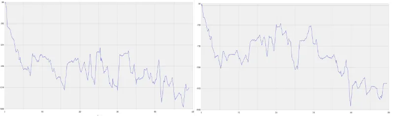
Figure 1. December 2015 expiration option prices, time value difference and ETF price trend.
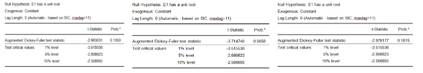
[image:3.595.99.498.386.479.2]Stationarity Test. Set the Shanghai 50ETF price as Y, the call option price as X1, and the put option price as X2.For example, the December 2015 combination.
Figure 2. Price stability test.
Under the confidence level of 0.05, the price of 50ETF, call options and put options are all zero order integrals, indicating that all three time series are stable. As for the June 2016 combination and the March 2017 combination, the situation is the same.
[image:3.595.93.507.607.679.2]Cointegration Test. The price of call option, put option and 50ETF are all stable. The precondition of arbitrage is that there is a long-term stable equilibrium relationship between the prices of the three, so it needs to carry out co-integration test. The three regressions are the return of the put option to the call option, the return of the ETF to the call option and the return of the put option to the ETF. For example, the December 2015 combination.
Figure 3. Co-integration test.
It can be seen from the test results that at the confidence level of 0.05, the residuals are all zero order integral. It shows that there is a long-term stable equilibrium relationship among the three variables. As for the June 2016 combination and the March 2017 combination, the situation is the same, there is a long-term stable equilibrium relationship among the three variables.
arbitrage strategy can be profitable on the premise of judging the correct price trend. Sell the subject matter and put options and buy the call option when the subject matter is short. The signal is required to be stable, not to be able to stop loss and gain in a timely manner, as long as it is guaranteed to filter out small consolidation areas and judge the general direction.
Figure 4. The yield curve.
A total of 112,000 yuan was invested from August 2015 to March 2017, with a maximum of 18,568 yuan being used. And net income of 16440 yuan, yield 14.68%.
[image:4.595.100.495.366.468.2]Comparison of Results between Different Periods and Pricing Options. On the daily line cycle, the profit and loss of holding position changes greatly, so try arbitrage on a 30-minute cycle, and also try arbitrage between different strike prices and different expiration months, and compare it with the arbitrage method above.
Figure 5. March 2016 the return of a 0.1/ 0.05 difference in the strike price.
Figure 6. Different months of the same strike price option feedback results.
As for the same month: the effect of 30 minutes was not good, and the benefit was -7990. As for the different month: the 30-minute period of the option with the same strike pricing for different months in March and June 2016 was selected for testing.
Summary
[image:4.595.100.499.499.617.2]return only contains the time value. When compared to 30 minutes, 30 minutes is not very profitable. And the effect of the same strike pricing option on different expiration months is not very different from that of the same strike pricing option on the same month. Due to the short position in the 30-minute time scale, the time value does not change enough time.
Although the research results are satisfactory, there are still many shortcomings and problems. For example, the judgment of the trend of the subject matter is purely random, which is closely related to the trading signal, so it is not a risk-free arbitrage in the strict sense.
Acknowledgement
Lu’s research was supported by the project of the National Social Science Foundation of China (no. 15BTJ016).
References
[1] Xian Jing-chen and Liu Qing. Research on options arbitrage paths and risk countermeasures of China's Shanghai a-share ETF [J], journal of Chongqing normal university (philosophical and social science edition), 2016, 5:76-85.
[2] Wang Kun. Research on option pricing, risk and arbitrage of Shanghai 50ETF [J], China prices, 2015, 9:42-45
[3] Zhu Wei. Application of option parity arbitrage in Chinese market [J], value engineering, 2016, 1:14-15.
[4] Sun Gui-ping, study on the effectiveness of cross-market arbitrage in CSI 300 index option simulation trading [J], business research, 2015 10(462).
[5] Jiang Xi-hua. Arbitrage opportunities in simulation trading of stock index options of csi 300 [N], futures daily, 2014-3-10(3).
[6] Han Jin. Application of vertical arbitrage strategy of domestic commodity options [N], futures daily, June 8, 2015 (3).
[7] Miao Miao. Study on stock index option simulation trading—a case study of DX futures company [D], Nanjing University of aeronautics and astronautics, 2016.