0 665
6 authors, including:
Some of the authors of this publication are also working on these related projects: COSMOSView project
EU H2020 Project RoMaNs: Robotic Manipulation for Nuclear Sort and SegregationView project Cheng Zhao University of Oxford 23PUBLICATIONS 192CITATIONS SEE PROFILE Kevin Li Sun University of Oxford 46PUBLICATIONS 520CITATIONS SEE PROFILE Zhi Yan
Université de Technologie de Belfort-Montbéliard
42PUBLICATIONS 580CITATIONS SEE PROFILE Tom Duckett University of Lincoln 214PUBLICATIONS 5,056CITATIONS SEE PROFILE
PII: S0921-8890(19)30154-X
DOI: https://doi.org/10.1016/j.robot.2019.07.004
Reference: ROBOT 3234
To appear in: Robotics and Autonomous Systems
Received date : 8 March 2019 Revised date : 1 July 2019 Accepted date : 8 July 2019
Please cite this article as:, Learning Kalman Network: A deep monocular visual odometry for on-road driving,Robotics and Autonomous Systems(2019), doi:
https://doi.org/10.1016/j.robot.2019.07.004.
This is a PDF file of an article that has undergone enhancements after acceptance, such as the addition of a cover page and metadata, and formatting for readability, but it is not yet the definitive version of record. This version will undergo additional copyediting, typesetting and review before it is published in its final form, but we are providing this version to give early visibility of the article. Please note that, during the production process, errors may be discovered which could affect the content, and all legal disclaimers that apply to the journal pertain.
Learning Kalman Network: A Deep Monocular
Visual Odometry for On-Road Driving
Cheng Zhao1, Li Sun2∗, Zhi Yan3, Gerhard Neumann3,
Tom Duckett3and Rustam Stolkin1
1Extreme Robotics Lab, University of Birmingham, UK.
2Oxford Robotics Institute, University of Oxford, UK.
3Lincoln Centre for Autonomous Systems, University of Lincoln, UK.
Abstract
This paper proposes a Learning Kalman Network (LKN) based monocular visual odometry (VO), i.e. LKN-VO, for on-road driving. Most existing learning-based VO focus on ego-motion estimation by comparing the two most recent consecutive frames. By contrast, the LKN-VO incorporates a learning ego-motion estimation through the current measurement, and a discriminative state estimator through a sequence of previous measurements. Superior to the model-based monocular VO, a more accurate absolute scale can be learned by LKN without any geomet-ric constraints. In contrast to the model-based Kalman Filter (KF), the optimal model parameters of LKN can be obtained from dynamic and deterministic out-puts of the neural network without elaborate human design. LKN is a hybrid approach where we achieve the non-linearity of the observation model and the transition model though deep neural networks, and update the state following the Kalman probabilistic mechanism. In contrast to the learning-based state estima-tor, a sparse representation is further proposed to learn the correlations within the states from the car’s movement behaviour, thereby applying better filtering on the 6DOF trajectory for on-road driving. The experimental results show that the proposed LKN-VO outperforms both model-based and learning state-estimator-based monocular VO on the most well-cited on-road driving datasets, i.e. KITTI and Apolloscape. In addition, LKN-VO is integrated with dense 3D mapping, which can be deployed for simultaneous localization and mapping in urban envi-ronments.
Keywords: Monocular Visual Odometry; Learning Kalman Filter; Vehicle
Driving
Journal
Pre-pro
of
A demonstrate video demo can be found on the link1.
1. Introduction
Simultaneous localization and mapping (SLAM) [1] is a core technique for self-driving cars [2] and mobile service robots [3][4]. Among the various SLAM methods developed for different sensor modalities, e.g. monocular [5], stereo [6], omnidirectional [7] camera, laser [8], lidar [9], etc., monocular SLAM is one of the most challenging due to its absolute scale drift problems and limitations in dense mapping.
Recently, deep-learning-based methods have provided new solutions for odometry[10], relocalization [11] and semantic mapping [12][13][14][15]. So far the
learning-based odometry approaches have mainly focused on monocular visual odome-try (VO) using supervised [16][10][17][18] or unsupervised [19][20][21][22] deep learning. They formulate visual localization as a regression problem, leveraging the ability of convolutional or recurrent neural networks. The main advantage of deep-learning-based monocular VO lies in rectifying the incorrect scale estima-tion of monocular SLAM.
Moreover, most of the learning-based approaches only focus on VO for local-ization without mapping. Prior work including CNN-SLAM [23], CodeSLAM [24] and DVSO [25] integrated deep-learning-based depth estimation with monocular SLAM methods to mitigate the weakness of dense mapping.
Most of the existing researches mainly focus on ego-motion estimation be-tween pairs of adjacent frames. However, trajectory refinement, which is usually based on filtering or optimization, is still an open problem for deep neural net-works [1]. The forerunner researches BKF [26] and LSTM-KF [27] proposed deterministic computation-graph-based filters for the state estimation.
In this paper, we propose a new Learning Kalman Network based monocular visual odometry (LKN-VO) with both ego-motion estimation and state estimation. In contrast to the previous learning-based methods mainly focusing on ego-motion estimation between adjacent frames, our LKN explores the ability of deep neural networks for state estimation to filter the 6DOF trajectory given a sequence of
1https://www.dropbox.com/s/k5a088hfjcpx9hy/RAS2019_1080.mp4?
dl=0
Journal
Pre-pro
of
measurements. This data-driven LKN can learn its dynamic changing parameters by end-to-end training, without specifying them explicitly.
Specifically, our proposed LKN includes the following new features: (i) a neural-network-based learning observation model can transform high-dimensional measurements to low-dimensional motion states to avoid modelling the full distri-bution over sensor readings; (ii) a neural-network-based learning transition model can model the non-linear transitions in the system dynamics; (iii) the uncertain-ties in the observation and transition models are formed in a sparse representation to learn the correlations within estimated states, which can provide a strong con-straint for the 6DOF trajectory filtering; and (iv) the Kalman Gain iteration is enhanced by a LSTM prior resulting in a more robust Kalman update.
The rest of this paper is organized as follows: First, related works are reviewed in Section 2. Then the proposed methods are introduced in Section 3 followed by experimental results and analyses in Section 4. Finally, we conclude the paper in Section 5. Supplementary materials are provided in Section 8.
2. Related work
In this section, we first review the recently supervised (Section 2.1) and un-supervised (Section 2.2) deep learning approaches for monocular VO. Then the latest achievements of deep-learning-based monocular VO with mapping are in-troduced in Section 2.3. Finally, the frontier researches on deep-learning-based trajectory filters/state estimators for monocular VO are reviewed in Section 2.4. 2.1. Supervised Deep Learning for Monocular VO
Deep-learning-based monocular VO can be grouped into supervised and un-supervised approaches. Supervised deep learning approaches formulate VO as a
regression problem. Costante et al. [28] first employed CNNs to estimate
ego-motion from the dense optical flow obtained by matching image features. Flow-Odometry [16] is the first end-to-end learning VO method, which combines FlowNet [29] for feature extraction with CNNs for regression. LS-VO [18] employs an auto-encoder network to find a non-linear representation of the optical flow manifold for ego-motion estimation. In contrast to model-based monocular VO, those re-searches achieve feature extraction and pose estimation by a non-linear CNN to directly regress the relative pose, and furthermore generate the global trajectory by accumulating relative poses.
DeepVO [30][10] leverages FlowNet features as the input of LSTM to learn
monocular VO as a sequence-to-sequence encoder-decoder. Clark
Journal
et. al [17]Pre-pro
of
use the same network architecture as [30][10] for RGB images but fused addi-tional IMU readings to improve the performance. GCN [31] also employed a CNN-RNN architecture to find the corresponding descriptors of keypoints. These monocular VO researches leverage the image interpretation ability of CNNs for descriptor learning and the sequential prediction ability of RNNs for state esti-mation. In contrast to conventional model-based VO, transforming optical flow directly to poses is a popular approach for deep-learning-based VO approaches such as DeepVO [30][10] based on learned optical flow features and LS-VO [18] based directly on learned optical flow.
In addition, some researches try to combine global and relative pose regres-sion through a shared neural network architecture, which can simultaneously per-form global relocalization and monocular VO. VLocNet [32] and its advanced version VLocNet++ [33] based on semantic knowledge can achieve 6DOF global pose regression and VO estimation from consecutive monocular images. Map-Net [34] learns a data-driven map representation for global camera localization – meanwhile it also learns the geometric constraint between two adjacent images to eliminate the drift in relative pose estimation. However, learning-based global relocalization can only be deployed in a known environment, and relative pose estimation plays an auxiliary role as a local geometry constraint. Hence, this cat-egory of monocular VO cannot be performed in an unknown environment.
Benefiting from the learning ability of CNNs and RNNs, the monocular VO based on supervised deep learning can estimate a more accurate absolute scale than conventional model-based monocular VO. Compared to conventional VO, a moderate amount of ground truth data is required for training a deep neural net-work. Despite this, the training data is relatively cheap to acquire than for many other learning tasks, e.g. semantic understanding, as the ground truth can be di-rectly obtained from GPS-RTK or Vicon cameras rather than manual annotations. 2.2. Unsupervised Deep Learning for Monocular VO
In order to eliminate the limitation of using ground truth trajectory, unsuper-vised deep monocular VO integrates geometric constraints, e.g. similarity con-straints, epipolar concon-straints, etc., into the loss function so that the deep neural network can be trained in an unsupervised way.
Most of the unsupervised methods jointly predict the depth and ego-motion si-multaneously using a geometric loss function. The forerunner work proposed by
Zhouet al.[19] can predict the depth and ego-motion simultaneously through a
training loss which minimizes the image warping error of an image sequence. An
extension of this work [35] adopted the same network architecture with a novel
Journal
Pre-pro
of
3D loss function based on geometric constraints to improve the performance. The multi-task networks SfM-Net [20], DeMoN [21] and GeoNet [36] can jointly pre-dict depth, segmentation, ego-motion, dense optical flow and surface normals us-ing an adaptive geometric consistency loss function.
Liet al.[22] and Zhanet al.[37] proposed similar approaches that combine
temporal (forward-backward) [19] and spatial (between left-right pairs) [38] loss
functions to achieve unsupervised monocular VO. Ganeshet al.[39] proposed a
loss function which can enforce geometric consistency of the trajectory so that the deep VO can be trained in an unsupervised way without additional stereo information. Using deep convolutional Generative Adversarial Networks (GANs), GANVO [40] can perform monocular VO with depth estimation. It proposed the minimization of warping view sequences and re-projection loss so that it can be trained in a generative unsupervised way.
These unsupervised deep monocular VO approaches are essentially not unsu-pervised approaches. To be specific, they still require additional information, such as consecutive frames or stereo images pairs instead of the ground truth trajectory, to provide the complementary supervision for the network training. Compared to supervised deep monocular VO, they usually require intrinsic parameters from the camera calibration and some of them using stereo images also need the extrinsic parameters of the stereo camera. Moreover, the performance of unsupervised deep VO is still inferior to that of supervised approaches.
2.3. Deep Learning for Monocular VO with Mapping
Model-based monocular SLAM struggles with dense mapping due to the lim-itations of depth prediction from the geometric inference. Most of the learning-based geometry research mainly focuses on odometry estimation, without includ-ing dense mappinclud-ing.
CNN-SLAM [23] is the first deep-learning-based SLAM system, which inte-grates deep depth prediction into LSD-SLAM to decrease the scale drift, mean-while generating a dense 3D map. Similarly, DVSO [25] also integrates self-supervised depth prediction based on StackNet into Direct Sparse Odometry [41] to obtain a sparse monocular SLAM method, which achieves very impressive re-sults. DeepTAM [42] is an entirely learned system for keyframe-based dense camera tracking and depth map estimation. They employ a multiple hypothesis approach for camera poses to enhance the camera pose tracking. Meanwhile, they employ cost volume information and image-based priors to enhance the dense depth estimation.
Journal
Pre-pro
of
Leveraging the latest achievements of learning-based dense depth prediction, the monocular SLAM problem can be formulated as virtual ‘RGB-D’ SLAM to alleviate the absolute scale drift issue and mitigate the limitations in dense map-ping. However, these approaches mainly employ deep learning to improve the depth prediction, while the other core components of the entire SLAM system, such as relocalization, loop closure and optimization, are still implemented using conventional geometry-based methods.
Frontier research Code-SLAM [24] first achieved a tight joint optimization of camera motion and dense depth prediction for dense monocular SLAM. How-ever, the dense 3D map generation and joint depth optimization can only be per-formed using limited numbers of keyframes in a very small scene. Our prelimi-nary work [43] proposed a learning monocular SLAM using dense 3D flow-based learning VO. A Bivariate Gaussian loss function is employed to learn the correla-tion between the mocorrela-tion direccorrela-tions. However, this research still considers monoc-ular VO as ego-motion estimation without trajectory filtering. The LKN-VO pre-sented in this paper provides significant novel technology beyond our previous work.
2.4. Deep Trajectory Filtering for Monocular VO
Most of the existing learning-based monocular VO mainly focuses on ego-motion learning using two adjacent images without global trajectory filtering. However, a probabilistic state estimator such as Kalman Filter or Particle Filter can filter the global trajectory to further improve the performance of VO using a sequence of measurements. To the best of our knowledge, there is limited litera-ture on deep-learning-based trajectory filtering for monocular VO. The following researches integrate the deep neural networks into the probabilistic filter frame-work as discriminative deterministic state estimators, which can be employed for monocular VO.
Backprop KF (BKF) [26] combines a Kalman Filter (KF) with a CNN-based observation model, which learns a non-linear mapping from the high-dimensional observation to the low-dimensional state. It can be trained in an end-to-end way using simple backpropagation through time. However, BKF assumes that the sys-tem dynamics are known and linear. For non-linear syssys-tems, additional approxi-mations, such as linearization of the system dynamics, are required.
LSTM-KF [27] integrates three LSTM units into the KF to learn the transition, observation and noise models. This method in the original paper is designed for temporal prediction problems, e.g. skeleton tracking, rather than VO. Due to the
Journal
Pre-pro
of
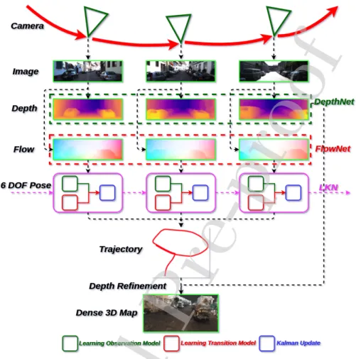
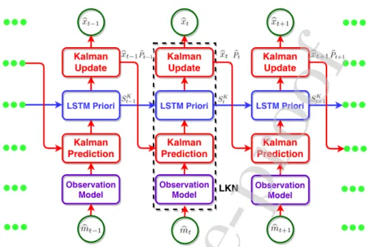
Figure 1: Pipeline of LKN-based deep monocular visual odometry with dense mapping. The LKN is enlarged in Figs. 2 and 3.
properties of LSTM, the learned representations depend on all previous observa-tions and states. However, these methods cannot model the correlaobserva-tions within the state variables as a result of using diagonal observation/transition covariance matrices. As shown in our experiments, modelling the correlations can provide a strong constraint for consecutive 6DOF pose estimation, and through which, the performance of monocular VO can be significantly improved.
Journal
Pre-pro
of
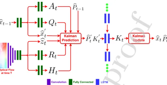
Figure 2: The architecture of LKN. The used symbol variables are defined in Eqs. (1) - (11). 3. Methodology
3.1. Overview
The pipeline of the proposed LKN-VO with 3D dense mapping is shown in Fig. 1. To be more specific, firstly the dense optical flow and depth are obtained using FlowNet2 [44] and DepthNet [38], respectively. Subsequently, the LKN si-multaneously estimates the ego-motion from current measurement and filters the states from a sequence of measurements. Consequently, a sequence of filtered states, i.e. 6 DOF relative poses, can be transformed to the global pose trajectory by the SE(3) composition layer [10]. Simultaneously, the point cloud is consis-tently generated from the estimated depth, and incrementally mapped with the learned global pose. Furthermore, an Octree depth fusion [43][45] is employed for a robust depth refinement, in which multi-view measurements are used to elim-inate inaccurate predictions. Finally, a dense 3D map can be obtained. As shown in Figs. 2 and 3, LKN is a computation graph made up of a Kalman Filter archi-tecture with learning observation and transition models, which can be trained as a complete graph from end to end. Please note that only monocular RGB images are employed for localization and mapping.
3.2. Learning Obvervation Model
The probabilistic filters are limited to handle rich sensor observations such
as images directly. An additional measurement model is usually required in or-
Journal
Pre-pro
of
Figure 3: Unrolled LKN architecture. The used symbol variables are defined in Eqs. (1) - (11).
der to avoid modelling the full distribution over sensor measurements. By con-trast, the observation model of LKN is designed using a deep neural network, which can transform the high-dimensional observations (e.g. RGB images) to low-dimensional states (e.g. 6DOF poses) directly. It is composed of the optical flow network and the ego-motion estimation network. FlowNet2 [44] is firstly em-ployed to predict the dense optical flow, which is of significant importance for the ego-motion learning. Then the ego-motion network can predict the 6DOF relative pose, observation matrix and noise covariance correspondingly.
More specially, in the model-based Kalman Filter, the observation zt of the
true statext at timetcan be obtained through a hand-designed observation matrix
Htand observation noise (rt) covarianceRt,
zt ,Htxt +rt, rt ∼N(0, Rt). (1)
By contrast, the non-linear observation model in LKN is approximated as a
deep neural networkh(Fig. 2) with learnable Gaussian noise,
b
zt, Ht, Rt =h(mt). (2)
Here, at time t, the raw measurement mt i.e. RGB images from the camera
are encoded by the deep neural networkhto the motion statebzt, i.e. 6 DOF pose.
Simultaneously, the observation matrix
Journal
Ht and observation noise covariance RtPre-pro
of
for the Kalman update are also learned by the deep neural networkh.
3.3. Learning Transition Model
The model-based Kalman Filter assumes that the statext is evolved from the
statext−1 through a hand-designed transition matrixAt and transition noise (qt)
covarianceQt,
xt ,Atxt−1+qt, qt ∼N(0, Qt). (3)
But in order to capture the motion changes in a non-linear dynamic system
(i.e. on-road driving), we use a deep neural networkf (Fig. 2) to approximate the
non-linear transition model with learnable Gaussian uncertainties,
b
x0t, At, Qt = f(bxt−1). (4)
At each time stampt, the intermediate statebx0t, which is not dependent on the
current measurement, can be produced by the neural networkf using the previous
state estimatebxt−1. Simultaneously, the transition matrixAt and transition noise
covarianceQt for the Kalman update are also learned by the neural networkf.
It is very complex to compute the Jacobian matrix of the non-linear function implemented by the deep neural network, and further linearize it by Taylor series.
Similar to the implementation of LSTM-KF2, we also employ a neural network to
approximate the transition matrixAtinstead of linearizing the functionf as in the
Extended Kalman Filter (EKF).
Furthermore, the prior state covariance matrixPbt0 at timetcan be updated as
b
Pt0 =AtPbt−1ATt +Qt. (5)
3.4. Sparse Representation
An intuitive hypothesis is that the motion correlations can be learned from the large-scale data collection of the car’s movement behaviors on the road. For example, there should be a hidden correlation between the linear and angular ve-locities for a car under different manoeuvres. In order to model the correlations between the main degree of freedom within the motion state, two sparse repre-sentation architectures are designed for the observation/transition matrices and observation/transition noise covariances. The sparse architectures enable LKN to learn both the uncertainties of the estimated states and the correlations within these states, which can be a significant constraint used for the trajectory filtering.
The transition/observation matricesA/Hare designed as
2https://github.com/Seleucia/lstmkf_ICCV2017/blob/master/
model_runner/klstm/kfl_QRFf.py
Journal
Pre-pro
of
A/H= A1/H1 0 A7/H7 0 A8/H8 0 0 A2/H2 0 0 0 0 A10/H10 0 A3/H3 0 A9/H9 0 0 0 0 A4/H4 0 0 A11/H11 0 A12/H12 0 A5/H5 0 0 0 0 0 0 A6/H6 . (6)
The transition/observation covariance matricesQ/Rare restricted to be
sym-metric positive definite,
Q/R= σx2 0 ρ1σxσz 0 ρ2σxσY 0 0 σ2 y 0 0 0 0 ρ1σxσz 0 σz2 0 ρ3σzσY 0 0 0 0 σ2 R 0 0 ρ2σxσY 0 ρ3σzσY 0 σY2 0 0 0 0 0 0 σP2 . (7)
Here, the coordinate design in this paper is the same as the KITTI camera
configuration3, i.e. the camera coordinate system is x : right (horizontal), y :
down (vertical), z :forward (horizontal). The 6DOF pose state is described as
(x, y, z, Roll, Y aw, P itch). We estimate six standard deviationsσx, σy, σz, σR, σY, σP
and three correlation coefficientsρ1, ρ2, ρ3 in the covariance matrices. ρ1 is the
correlation coefficient of the states xand z. ρ2 is the correlation coefficient of
the states x and Y(Y aw). ρ3 is the correlation coefficient of the states z and
Y(Y aw). For the on-road driving, the states x (horizontal), z (horizontal) and
Y(rotation around y) are the main translational and rotational degrees of freedom.
Intuitively, we only need to find the cross-correlations between statesx,zandY.
3.5. LSTM Prior
Using the prior state covariancePbt0 from the Kalman prediction, an
intermedi-ate Kalman GainKt0 at timetis calculated as
Kt0 =Pbt0HT t (HtPb
0
tHtT +Rt)−1. (8)
We further use the intermediate Kalman GainKt0 as the observation input of
a Long Short-Term Memory (LSTM) stack. It can learn the transition of Kalman
3http://www.cvlibs.net/datasets/kitti/setup.php
Journal
Pre-pro
of
Gains in a hidden state space from high-dimensional stateSK
t−1 toStK, which can
provide additional prior knowledge for Kalman GainKt estimation,
Kt, StK =LST Mn(K
0
t, StK−1). (9)
Here,nis the number of LSTM cells. It is worth noting that, provided sparse
representations of the transition/observation matrices and the corresponding co-variance matrices, the intermediate Kalman Gain is also a sparse matrix after a series of matrix operations. We only apply the LSTM stack to regress the
non-zero elements in the sparse matrix (12 non-non-zero elements in the 6×6 matrix) in
order to protect the inherent sparse architecture.
Unlike the model-based KF, the transition/observation matrices and the cor-responding covariance matrices in LKN are dynamically changing through time. The LSTM prior can learn to memorize and forget the previous high-dimensional states of the Kalman Gain in the hidden state space, which allows for a more robust iteration and convergence of the Kalman Gain.
3.6. Kalman Update
Finally, in the Kalman update procedure, the final prediction bxt at timet can
be inferred analytically from the intermediate states, covariance estimations and Kalman Gain, b xt =bx 0 t+Kt(zbt−Htxb 0 t). (10)
The posterior state covariance matrixPbtat timetcan be updated as
b
Pt = (I−KtHt)Pb
0
t(I−KtHt)T +KtRtKtT. (11)
To facilitate the reader’s understanding of the proposed method, we explicitly
indicate the dimension of each symbol variable (matrix) in Eqs. (1) - (11):zbt,xb
0
t,
b
xt are 6 dimensional,Ht,At, Rt,Qt are 6×6 dimensional,Pb
0 t, Pbt,K 0 t,Kt, Iare 6×6 dimensional andSK t are 128 dimensional. 3.7. Network Architecture
The learning observation network is composed of an optical flow network, i.e. Flownet2, and ego-motion estimation network. The ego-motion estimate network includes a convolution stack, with three branches of fully-connected stacks. In order to keep the spatial geometry information, the pooling layer is abandoned in
the convolution stack. The convolution layers are composed of3×3filters with a
stride of2. Its number of channels are64, 128, 256and512withreluactivation
function. A sequence of fully-connected regressors constitute the fully-connected
stack. The hidden state of the regressors is set to
Journal
128withreluactivation function.Pre-pro
of
The learning transition network is composed of three branches of fully-connected stacks. A sequence of fully-connected regressors constitute the fully-connected
stack. The hidden state of the regressors is set to128withrelu activation
func-tion. The LSTM stack comprises two standard LSTM cells with a hidden state of
128. The detail architecture and parameters of observation, transition and LSTM
prior networks are shown in the Section 8.3. 3.8. Loss Function and Optimization
The standard Euclidean`2loss is employed for the loss function optimization.
Similar to [30], the Euler Angles are used to represent the orientation. We further
include a`2 regularization term for all trainable weights to mitigate against
over-fitting. Our loss function is defined as
loss=λ1 N X i n X j kTpi,j−Tgti,jk2+λ2 N X i n X j kRi,jp −Ri,jgtk2+λ3kWk2, (12)
wherenis the length of the observation sequences, andN is the number of
train-ing sequences. Ti,j
p := (xp, yp, zp)i,j and Tgti,j := (xgt, ygt, zgt)i,j are the
pre-dicted and ground truth camera translation, respectively.Ri,j
p := (ezp, eyp, exp)i,jand
Ri,jgt := (ez
gt, eygt, exgt)i,j are the predicted and ground-truth rotation in Euler
An-gles, respectively. W represents the trainable weights of the neural network. λ1,
λ2 and λ3 are the scaling factors to balance the weights of translation and
rota-tion loss, which are set according to practical experience. The Adam Optimizer is employed to optimize all the trainable parameters to minimize the loss function.
4. Experiments
The KITTI4odometry benchmark is employed for the LKN evaluation, which
consists of 22 sequences of saved RGB images in PNG format. Accurate 6 DOF
ground truth trajectories (< 10cm) from a GPS/IMU system are provided for
the sequences 00-10. There are no ground truth trajectories available for the se-quences 11-21, but an online submission portal for evaluation is provided.
More-over, the Apolloscape5self-localization dataset is also employed as a
supplemen-tary evaluation in order to further verify the generalization ability of LKN.
4http://www.cvlibs.net/datasets/kitti/eval_odometry.php
5http://apolloscape.auto/self_localization.html
Journal
Pre-pro
of
4.1. Network Training
During training, the network is trained for 300 epochs with a batch size of
100. The step learning policy is employed and the learning rate decay is fixed to
0.95. The starting learning rate is10−4 and minimum learning rate is10−7. The
momentum is fixed to (0.9,0.999). The scaling factors are set to λ1=1, λ2=1e3
andλ3=1e-3 correspondingly. The start time-point of a sub-sequence is randomly
selected from the whole sequence and the length of each sub-sequence is set to 10. The algorithm computes the gradient by rolling from the random start point to the end of the whole sequence. Gradient clipping is used in order to increase the training robustness.
Considering the GPU limitation and the nearly real-time running requirement for the SLAM system, the raw RGB images from the KITTI dataset are
down-sampled 4 times to 320× 96, although the performance will degrade using a
smaller image size. Thus there is a trade-off between runtime and performance. The whole network is end-to-end trainable, while training it step-by-step is more practicable because of the computing resource limitation. The weights of the ego-motion estimation network, the transition network and the LSTM stack are opti-mized while the weights of Flownet2 are frozen.
In addtion, we fine-tune the FlowNet2 [44] and DepthNet [38] using the KITTI training data (as described in 4.3) and then transplant them for our task. Follow-ing [29][38] and [10], both image augmentation (color, brightness, gamma) and geometric augmentation (translation, rotation, scaling) are used to enhance per-formance and mitigate overfitting.
4.2. Baselines
For a comparable evaluation, the performances of 7 different baselines (B1...B7)
are provided.B1andB2are employed to compare with the conventional
model-based VO.B4and B5are employed to compare with the LSTM-based state
es-timator. B3, B6 and B7 are employed to compare with the model-based and
learning-based KF for state estimation.
• VISO-S (B1) and VISO-M (B2) [6] are the geometry-feature-based stereo
and monocular VO in the open source VO library VISO26, which are
tai-lored VO for the self-driving car. In order to eliminate the absolute scale drift, the height and pitch are fixed to 1.7 and -0.03 for VISO-M according to the author’s suggestions for the KITTI dataset.
6http://www.cvlibs.net/software/libviso/
Journal
Pre-pro
of
• BKF [26] (B3) proposed a learning observation model using the
differ-ence image, which can approximate the non-linear observation mapping with noise covariance by neural networks. It integrates a CNN-based obser-vation model with KF to learn a non-linear transformation from the high-dimensional image to the low-high-dimensional motion state through end-to-end training. The system dynamics is assumed to be known and linear. Other-wise, an additional model-based EKF is required for the linearization of the system dynamics.
• ESP-VO [10] (B4) and LSTMs (B5) are both LSTM-based learning
monoc-ular VO. The former employs the observation model also based on the opti-cal flow feature as in the original paper, while the latter (re-implemented by ourselves) employs the observation model proposed in our LKN approach. They are sequence-to-sequence encoder-decoder, which leverages the ad-vantage of the variance perception ability of FlowNet for the descriptor learning and the prediction ability of LSTM for the state estimation.
• Conventional KF (B6) represents the model-based filter approach. It
em-ploys the observation model proposed in our LKN approach to transform the high-dimensional sensor measurement to the low-dimensional motion state, so that the KF can filter a sequence of states. Its parameters are hand-designed according to experience, and not learned by the neural network. The parameters are the same with parameter settings of the baseline in the
LSTM-KF7.
• LSTM-KF [27] (B7) uses three LSTM units to model the transition
func-tion and the transifunc-tion/observafunc-tion noise covariance. It leverages LSTM to make the representations depend on all previous observations and all pre-vious states. However, its covariance matrices are simplified as diagonal matrices, which cannot learn the correlations within the motion states. It is designed for skeleton tracking in the original paper rather than the VO
problem. Therefore we re-implemented it based on their open-source code8
with the observation model proposed in our LKN approach and tested it on the public datasets.
7https://github.com/Seleucia/lstmkf_ICCV2017/blob/master/ model_runner/klstm/kf_tf.py 8https://github.com/Seleucia/lstmkf_ICCV2017
Journal
Pre-pro
of
• Note: For a fair comparison, we provide the state estimator baselines B5,
B6and B7with the proposed learning observation model (the same with
our LKN) for the ego-motion estimation. For the non-open-source baselines B3 (BKF) and B4 (ESP-VO), the experimental results are cited from their original paper.
4.3. Evaluation of Visual Odometry on KITTI Dataset
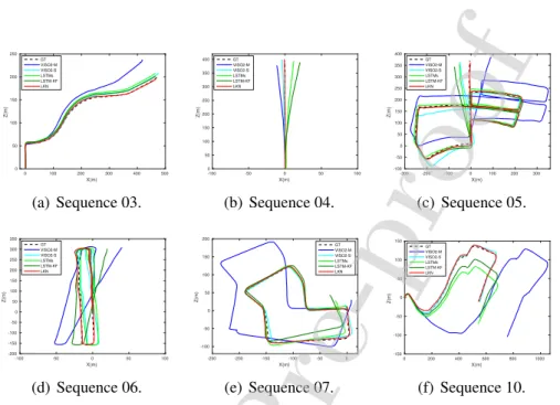
Two kinds of evaluations are employed to compare the proposed LKN to base-lines. Following the same partition in [10] for a fair comparison, the first evalua-tion uses sequences 00-10 and is split to 00, 01, 02, 08, 09 for training and 03, 04, 05, 06, 07, 10 for testing. The second evaluation uses sequences 21 where 00-10 are used for training and 11-21 for testing. For a direct display, the trajectories generated by LOAM [46] are provided as the reference in the second evaluation because no ground truth data are provided. LOAM achieves the-state-of-the-art performance using 3D Lidar data on the KITTI odometry benchmark. The stan-dard KITTI VO evaluation metrics, i.e., computing the average translational and
rotational RMSE for all possible sub-sequences of length(100, . . . ,800)meters,
are employed as evaluation criteria.
For the first evaluation, the overall average translational and rotational errors
of LKN are1.79%and0.87◦/100mrespectively. The comparisons of qualitative
performances are shown in Fig. 4. The quantitative results are shown in Fig. 6 for different length/speed analysis, Table 1 for subsequence analysis and Table 2 for ablation analysis.
Table 1: The comparison of performance of LKN against the baselines on the KITTI dataset according to the evaluation method [10]. Note that VISO-S is a stereo VO and the other methods are monocular VO. The learning model is trained on the sequences 00, 01, 02, 08 and 09, and evaluated on the rest. Some results are copied from [26] and [10].
Seq. (1242VISO-S[6]×376) (1242VISO-M[6]×376) (150BKF [26]×50) ESP-VO[10](1241×376) (320LSTMs×96) (320KF×96) LSTM-KF [27](320×96) (320LKN×96)
trel(%) rrel(◦) trel(%) rrel(◦) trel(%) rrel(◦) trel(%) rrel(◦) trel(%) rrel(◦) trel(%) rrel(◦) trel(%) rrel(◦) trel(%) rrel(◦)
03 1.71 1.12 9.02 2.83 - - 6.72 6.46 3.09 1.76 3.62 2.05 3.30 1.85 3.25 1.41 04 1.54 0.84 4.33 1.63 - - 6.33 6.08 2.24 1.09 2.94 1.74 2.82 1.62 1.40 0.51 05 2.36 1.20 19.16 3.62 - - 3.35 4.93 2.91 1.24 3.24 1.33 3.13 1.31 1.39 0.61 06 1.47 0.87 6.64 1.96 - - 7.24 7.29 2.41 0.91 2.18 1.14 1.84 1.03 1.46 0.80 07 2.37 1.78 26.54 5.92 - - 3.52 5.02 4.22 2.70 6.09 3.78 5.97 3.78 2.51 1.87 10 1.51 1.15 48.29 3.43 - - 9.77 10.2 3.79 1.51 4.03 1.54 3.54 1.46 2.68 1.13 Mean 1.83 1.16 19.00 3.23 - - 6.15 6.66 3.11 1.54 3.68 1.93 3.43 1.84 2.11 1.05 Overall 2.05 1.19 21.00 3.46 18.04 5.56 - - 3.07 1.38 3.45 1.60 3.24 1.55 1.79 0.87
trel(%)andrrel(◦)are average translational RMSE(%) and rotational RMSE(◦/100m) over100m−800mintervals.
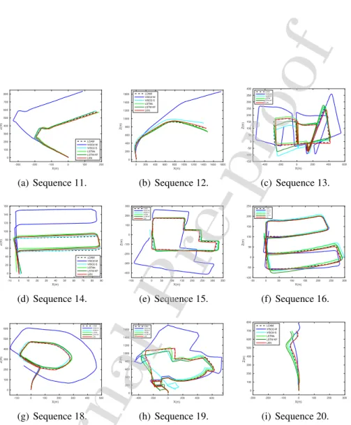
In the second evaluation, the overall average translational and rotational errors
of LKN are2
Journal
.66%and0.79◦/100m, respectively, obtained with the KITTI onlinePre-pro
of
X(m) 0 100 200 300 400 500 Z(m) 0 50 100 150 200 250 GT VISO2-M VISO2-S LSTMs LSTM-KF LKN (a) Sequence 03. X(m) -100 -50 0 50 100 Z(m) 0 50 100 150 200 250 300 350 400 GT VISO2-M VISO2-S LSTMs LSTM-KF LKN (b) Sequence 04. X(m) -300 -200 -100 0 100 200 300 Z(m) -100 -50 0 50 100 150 200 250 300 350 400 GT VISO2-M VISO2-S LSTMs LSTM-KF LKN (c) Sequence 05. X(m) -100 -50 0 50 100 Z(m) -200 -150 -100 -50 0 50 100 150 200 250 300 350 GT VISO2-M VISO2-S LSTMs LSTM-KF LKN (d) Sequence 06. X(m) -250 -200 -150 -100 -50 0 Z(m) -100 -50 0 50 100 150 200 GT VISO2-M VISO2-S LSTMs LSTM-KF LKN (e) Sequence 07. X(m) 0 200 400 600 800 1000 Z(m) -150 -100 -50 0 50 100 150 GT VISO2-M VISO2-S LSTMs LSTM-KF LKN (f) Sequence 10.
Figure 4: The predicted trajectories of LKN on the sequences 03, 04, 05, 06, 07 and 10 from the KITTI dataset. The learning model is trained on the sequences 00, 01, 02, 08 and 09.
Table 2: The ablation analysis for the performance of LKN. B: learning ego-motion estimation with model-based KF (manually designed parameters). L: learning non-linear observation/transi-tion models. S: sparse representaobservation/transi-tion. P: LSTM Prior.
Architecture trel(%) rrel(◦)
B 3.42 1.64
B+L 3.01 1.41
B+L+S 2.03 0.99
B+L+S+P 1.79 0.87
trel(%)andrrel(◦/100m)are the same as in Table 1.
Journal
Pre-pro
of
X(m) -300 -200 -100 0 100 200 Z(m) 0 100 200 300 400 500 600 700 800 LOAM VISO2-M VISO2-S LSTMs LSTM-KF LKN (a) Sequence 11. X(m) 0 200 400 600 800 10001200140016001800 Z(m) 0 200 400 600 800 1000 1200 1400 1600 LOAM VISO2-M VISO2-S LSTMs LSTM-KF LKN (b) Sequence 12. X(m) -400 -200 0 200 400 600 Z(m) -150 -100 -50 0 50 100 150 200 250 300 350 400 LOAM VISO2-M VISO2-S LSTMs LSTM-KF LKN (c) Sequence 13. X(m) -10 0 10 20 30 40 50 60 70 80 90 Z(m) 0 20 40 60 80 100 120 140 160 LOAM VISO2-M VISO2-S LSTMs LSTM-KF LKN (d) Sequence 14. X(m) -100 -50 0 50 100 150 200 250 300 350 Z(m) -400 -300 -200 -100 0 100 200 300 LOAM VISO2-M VISO2-S LSTMs LSTM-KF LKN (e) Sequence 15. X(m) -50 0 50 100 150 200 250 300 Z(m) -100 -50 0 50 100 150 200 250 LOAM VISO2-M VISO2-S LSTMs LSTM-KF LKN (f) Sequence 16. X(m) -100 0 100 200 300 400 500 Z(m) 0 100 200 300 400 500 600 LOAM VISO2-M VISO2-S LSTMs LSTM-KF LKN (g) Sequence 18. X(m) -400 -200 0 200 400 600 Z(m) 0 200 400 600 800 1000 1200 1400 1600 LOAM VISO2-M VISO2-S LSTMs LSTM-KF LKN (h) Sequence 19. X(m) -300 -200 -100 0 100 200 300 Z(m) 0 100 200 300 400 500 600 700 800 LOAM VISO2-M VISO2-S LSTMs LSTM-KF LKN (i) Sequence 20.
Figure 5: The predicted trajectories of LKN on the sequences 11, 12, 13, 14, 15, 16, 18, 19 and 20 from the KITTI dataset. The network is trained on the sequences 00-10. The trajectories generated by LOAM [46] are provided as the reference.
Journal
Pre-pro
of
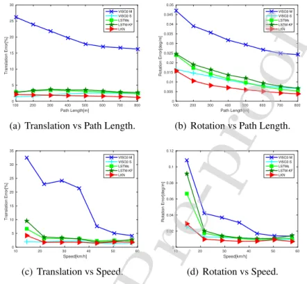
Path Length[m] 100 200 300 400 500 600 700 800 Translation Error[%] 0 5 10 15 20 25 30 VISO2-M VISO2-S LSTMs LSTM-KF LKN
(a) Translation vs Path Length.
Path Length[m] 100 200 300 400 500 600 700 800 Rotation Error[deg/m] 0 0.005 0.01 0.015 0.02 0.025 0.03 0.035 0.04 0.045 0.05 VISO2-M VISO2-S LSTMs LSTM-KF LKN
(b) Rotation vs Path Length.
Speed[km/h] 10 20 30 40 50 60 Translation Error[%] 0 5 10 15 20 25 30 35 VISO2-M VISO2-S LSTMs LSTM-KF LKN (c) Translation vs Speed. Speed[km/h] 10 20 30 40 50 60 Rotation Error[deg/m] 0 0.02 0.04 0.06 0.08 0.1 0.12 VISO2-M VISO2-S LSTMs LSTM-KF LKN (d) Rotation vs Speed.
Figure 6: Average translational and rotational errors of LKN against different path lengths and speeds. The learning model is trained on the sequences 00, 01, 02, 08 and 09, and evaluated on the rest.
submission portal. The comparison of qualitative results is shown in Fig. 5. The methods with closer trajectories to LOAM can be regarded as superior. More details about the quantitative results of the second evaluation can be found in
Section 8.1 or KITTI odometry online evaluation website9.
From Table 2, it can be seen that the performance improvement of LKN mainly comes from three parts: the learning non-linear observation/transition models, the sparse representation and the LSTM prior.
From the comparison, we can see the performance of LKN is superior to model-based monocular VO, and is even comparable with a model-based stereo VO (VISO2-M). The model-based monocular VO (without dense depth
predic-9http://www.cvlibs.net/datasets/kitti/eval_odometry_detail.
php?&result=e2b9434f9bd33770c66680871e8262990d0a780a
Journal
Pre-pro
of
tion and loop detection) suffers from absolute scale drift, while the learning-based methods can learn a more accurate absolute scale without any scene-based geo-metric constraints such as camera height, which is the main reason why LKN can significantly outperform model-based monocular VO.
We can also see that LKN outperforms BKF and ESP-VO. We believe that one reason for this is the improved learning observation model used in the LKN. Moreover, BKF requires an additional model-based EKF for the non-linear system approximation rather than learning from data. Using the same learning observa-tion model for ego-moobserva-tion estimaobserva-tion, LKN also achieves a better performance than the conventional KF, LSTM-KF and LSTMs. Compared to the conventional KF, LKN can learn the non-linear transition/observation models with the corre-sponding noise covariances instead of specifying them manually. Comparing with the LSTM-KF and LSTMs, LKN can learn the sparse covariance matrices, rather than the simple diagonal matrix used in LSTM-KF and provide a more principled treatment of uncertainty than the LSTMs. It can model the correlations within the motion states as a strong constraint for the 6DOF trajectory filtering. Moreover, the LSTM prior in LKN is helpful for the Kalman Gain iteration for a more robust Kalman update.
4.4. Evaluation of Visual Odometry on Apolloscape Dataset
To further verify the generalization ability of the LKN, the Apolloscape
self-localization dataset10is employed for additional evaluation. The Apolloscape
self-localization dataset consists of 151 sequences from 6 different roads (28km) in 4
different cities. It provides roughly300k RGB images saved as JPG format and
accurate 6 DOF (translation≤ 50mm, rotation≤0.015◦ ) ground truth
trajecto-ries from a GPS/IMU system. The evaluation metrics provided by the Apolloscape self-localization dataset, i.e., median translation offset and median relative angle, are used for global localization, not for odometry. So the standard KITTI odom-etry evaluation metrics, i.e., computing the average translational and rotational
RMSE for all possible sub-sequences of length (100, . . . ,800) meters, are also
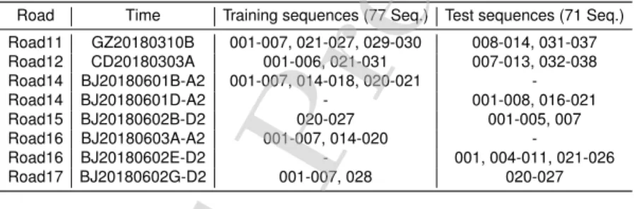
employed as evaluation criteria. The 151 sequences from 6 different roads are split into 77 sequences for training and 71 sequences for testing. Three sequences are abandoned because only one image was included in these sequences. The training and test sequences are split as shown in Table 3.
As mentioned in the paper, three learning based state estimators, i.e. BKF [26],
10http://apolloscape.auto/self_localization.html
Journal
Pre-pro
of
ESP-VO [10] and LSTM-KF [27] are our main baseline approaches. The author of BKF did not release their code, so it is difficult to implement it in a short time to provide the evaluation results on the Apolloscape dataset. ESP-VO combines CNN with LSTMs, and LSTM-KF is an open-source approach. We implemented them with the observation model proposed in our LKN approach for a fair compar-ison. The comparison quantitative results on the Apolloscape dataset are reported in Table 4. We also provide some selected qualitative results of LKN in Fig. 10 in Section 8.2. Comparing with the main baselines, the improvement from LKN on the Apolloscape dataset is less than that on the KITTI dataset. The main reason is that the testing sequences from the Apolloscape dataset are less challenging than those from the KITTI dataset. The trajectories in the former dataset usually have at most one corner, as shown in Fig. 10, while the trajectories in the latter dataset are usually more curved, as shown in Fig. 4 and Fig. 5.
Table 3: The split training and test sequences on the Apolloscape dataset.
Road Time Training sequences (77 Seq.) Test sequences (71 Seq.)
Road11 GZ20180310B 001-007, 021-027, 029-030 008-014, 031-037 Road12 CD20180303A 001-006, 021-031 007-013, 032-038 Road14 BJ20180601B-A2 001-007, 014-018, 020-021 -Road14 BJ20180601D-A2 - 001-008, 016-021 Road15 BJ20180602B-D2 020-027 001-005, 007 Road16 BJ20180603A-A2 001-007, 014-020 -Road16 BJ20180602E-D2 - 001, 004-011, 021-026 Road17 BJ20180602G-D2 001-007, 028 020-027
Table 4: The comparison of performance of LKN against main baselines on the Apolloscape dataset.
Road (Seq. amount) ESP-VO/LSTMs [10](416×336) LSTM-KF [27](416×336) (416LKN×336)
trel(%) rrel(◦) trel(%) rrel(◦) trel(%) rrel(◦)
Road11 (14 Seq.) 1.61 0.86 1.65 0.88 1.41 0.70 Road12 (14 Seq.) 1.99 1.05 1.39 0.71 1.10 0.56 Road14 (14 Seq.) 1.82 0.99 2.01 0.93 1.67 0.82 Road15 ( 6 Seq.) 2.02 1.16 1.97 0.92 1.40 0.73 Road16 (15 Seq.) 1.77 0.78 1.70 0.73 1.53 0.65 Road17 ( 8 Seq.) 2.71 0.96 2.99 1.06 1.46 0.60
trel(%)andrrel(◦)are average translational RMSE(%) and rotational RMSE(◦/100m) over100m−800mintervals.
Journal
Pre-pro
of
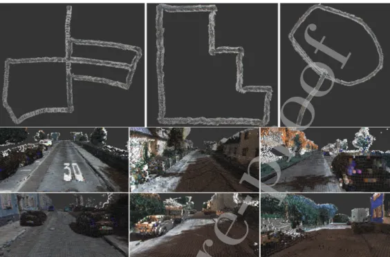
Figure 7: The first row depicts the global dense 3D maps of sequences 05, 15 and 18 from the KITTI dataset. The small images in the second and third row show enlarged local areas of the global map.
4.5. Dense 3D Mapping
We integrated LKN-VO with dense 3D mapping, which is implemented under
the ROS11 framework. The LKN implemented by Tensorflow12 is trained on an
NVIDIA Titan GPU accelerated by CUDA and CUDNN. As shown in Fig. 7, the
images on the first row show the global dense 3D map of sequences05,15and18
on the KITTI dataset and the images on the second and third row show enlarged local areas of the global map. The Octree depth fusion [43][45] with multi-view measurements associated by LKN can alleviate the border blur and remove many outliers arising from inaccurate depth predictions from a single frame. It can be seen that the more sharply defined shapes such as the car, trees and buildings can be generated after depth fusion.
11http://www.ros.org/
12https://www.tensorflow.org/
Journal
Pre-pro
of
5. Conclusion, Limitation and Future work
This paper proposed a discriminative state-estimator-based monocular VO ap-proach, LKN-VO, to simultaneously estimate the ego-motion and filter the tra-jectory for on-road driving. Our main contribution is the proposed hybrid LKN model that combines the non-linear transform property of data-driven deep neural networks with the probabilistic fusion mechanism of the Kalman Filter. Com-paring with the model-based monocular VO, LKN-VO can learn a more accurate absolute scale without the requirement of scene-based geometric constraints for the trajectory. In contrast to the model-based KF, LKN is a deterministic KF-based computation graph, in which the non-linear observation and transition mod-els with noise uncertainties are approximated through neural networks. In contrast to the existing learning state estimators, the sparse representation (modelling cor-relations within state dimensions) and the LSTM prior in LKN can provide more powerful spatio-temporal constraints for the trajectory filtering. The performance of LKN-VO exceeds that of the model-based and learning state-estimator-based monocular VO on the most well-cited self-driving datasets, i.e. KITTI and Apol-loscape. Last, but not least, the LKN-VO is able to perform simultaneous lo-calization and mapping in urban environments, via the integration of dense 3D mapping.
The common limitation of deep-learning-based localization and mapping is its high computational requirement. One potential solution is to learn smaller and shallower but ‘good enough’ neural networks via model dilation and then deploy them via on-board GPU devices such as NVIDIA DRIVE AGX. For future work, we will investigate the possibility to integrate deep-learning-based loop closure into the proposed system to establish a globally consistent representation of the environment. In that case, graph optimization can be performed to significantly mitigate the trajectory drift with the error accumulation from VO. Lastly, with the rapid development of coming high-speed 5G communication technologies, we will investigate a service-client mode based on 5G to mitigate the high computa-tional requirement of the proposed method as an on-board system.
6. Acknowledgement
This work was funded by DISTINCTIVE scholarship and EU H2020 projects ILIAD (732737) & RoMaNS (645582).
Journal
Pre-pro
of
7. References
[1] C. Cadena, L. Carlone, H. Carrillo, Y. Latif, D. Scaramuzza, J. Neira, I. Reid, J. Leonard, Past, present, and future of simultaneous localization and map-ping: Towards the robust-perception age, IEEE Transactions on Robotics 32 (6) (2016) 13091332 (2016).
[2] G. Xie, H. Gao, L. Qian, B. Huang, K. Li, J. Wang, Vehicle trajectory pre-diction by integrating physics-and maneuver-based approaches using inter-active multiple models, IEEE Transactions on Industrial Electronics 65 (7) (2018) 5999–6008 (2018).
[3] C. Zhao, W. Mei, W. Pan, Building a grid-semantic map for the navigation of service robots through human-robot interaction, Digital Communications and Networks 1 (4) (2015) 253–266 (2015).
[4] C. Zhao, H. Hu, D. Gu, Building a grid-point cloud-semantic map based on graph for the navigation of intelligent wheelchair, in: IEEE International Conference on Automation and Computing, IEEE, 2015, pp. 1–7 (2015). [5] L. An, X. Zhang, H. Gao, Y. Liu, Semantic segmentation aided visual
odometry for urban autonomous driving, International Journal of Advanced Robotic Systems 14 (5) (2017) 1729881417735667 (2017).
[6] A. Geiger, J. Ziegler, C. Stiller, StereoScan: Dense 3d reconstruction in real-time, in: Intelligent Vehicles Symposium, IEEE, 2011, pp. 963–968 (2011). [7] F. Dayoub, T. Duckett, An adaptive appearance-based map for long-term topological localization of mobile robots, in: IEEE/RSJ International Con-ference on Intelligent Robots and Systems, IEEE, 2008, pp. 3364–3369 (2008).
[8] H. Andreasson, T. Duckett, A. J. Lilienthal, A minimalistic approach to appearance-based visual slam, IEEE Transactions on Robotics 24 (5) (2008) 991–1001 (2008).
[9] H. Gao, B. Cheng, J. Wang, K. Li, J. Zhao, D. Li, Object classification using cnn-based fusion of vision and lidar in autonomous vehicle environ-ment, IEEE Transactions on Industrial Informatics 14 (9) (2018) 4224–4231
(2018).
Journal
Pre-pro
of
[10] S. Wang, R. Clark, H. Wen, N. Trigoni, End-to-end, sequence-to-sequence probabilistic visual odometry through deep neural networks, The Interna-tional Journal of Robotics Research (2017).
[11] P. Purkait, C. Zhao, C. Zach, Spp-net: Deep absolute pose regression with synthetic views, arXiv preprint arXiv:1712.03452 (2017).
[12] C. Zhao, L. Sun, R. Stolkin, A fully end-to-end deep learning approach for real-time simultaneous 3d reconstruction and material recognition, in: IEEE International Conference on Advanced Robotics, IEEE, 2017, pp. 75– 82 (2017).
[13] C. Zhao, L. Sun, P. Purkait, T. Duckett, R. Stolkin, Dense rgb-d seman-tic mapping with pixel-voxel neural network, Sensors 18 (9) (2018) 3099 (2018).
[14] L. Sun, Z. Yan, A. Zaganidis, C. Zhao, T. Duckett, Recurrent-octomap: Learning state-based map refinement for long-term semantic mapping with 3-d-lidar data, IEEE Robotics and Automation Letters 3 (4) (2018) 3749– 3756 (2018).
[15] L. Sun, C. Zhao, R. Stolkin, Weakly-supervised dcnn for rgb-d object recog-nition in real-world applications which lack large-scale annotated training data, arXiv preprint arXiv:1703.06370 (2017).
[16] P. Muller, A. Savakis, Flowdometry: An optical flow and deep learning based approach to visual odometry, in: IEEE Winter Conference on Applications of Computer Vision, 2017, pp. 624–631 (2017).
[17] R. Clark, S. Wang, H. Wen, A. Markham, N. Trigoni, VINet: Visual-inertial odometry as a sequence-to-sequence learning problem., in: The AAAI Con-ference on Artificial Intelligence, 2017, pp. 3995–4001 (2017).
[18] G. Costante, T. A. Ciarfuglia, LS-VO: Learning dense optical subspace for robust visual odometry estimation, IEEE Robotics and Automation Letters 3 (3) (2018) 1735–1742 (2018).
[19] T. Zhou, M. Brown, N. Snavely, D. G. Lowe, Unsupervised learning of depth and ego-motion from video, in: IEEE Conference on Computer Vision and
Pattern Recognition, Vol. 2, 2017, p. 7 (2017).
Journal
Pre-pro
of
[20] S. Vijayanarasimhan, S. Ricco, C. Schmid, R. Sukthankar, K. Fragkiadaki, SfM-Net: Learning of structure and motion from video, arXiv preprint arXiv:1704.07804 (2017).
[21] B. Ummenhofer, H. Zhou, J. Uhrig, N. Mayer, E. Ilg, A. Dosovitskiy, T. Brox, DeMoN: Depth and motion network for learning monocular stereo, in: IEEE Conference on Computer Vision and Pattern Recognition, Vol. 5, 2017 (2017).
[22] R. Li, S. Wang, Z. Long, D. Gu, UnDeepVO: Monocular visual odometry through unsupervised deep learning, in: IEEE International Conference on Robotics and Automation, IEEE, 2018, pp. 7286–7291 (2018).
[23] K. Tateno, F. Tombari, I. Laina, N. Navab, CNN-SLAM: Real-time dense monocular slam with learned depth prediction, in: Proceedings of the IEEE Conference on Computer Vision and Pattern Recognition, 2017, pp. 6243– 6252 (2017).
[24] M. Bloesch, J. Czarnowski, R. Clark, S. Leutenegger, A. J. Davison, CodeSLAM - learning a compact, optimisable representation for dense vi-sual slam, in: IEEE Conference on Computer Vision and Pattern Recogni-tion, 2018, pp. 2560–2568 (2018).
[25] N. Yang, R. Wang, J. Stuckler, D. Cremers, Deep virtual stereo odometry: Leveraging deep depth prediction for monocular direct sparse odometry, in: European Conference on Computer Vision, 2018, pp. 817–833 (2018). [26] T. Haarnoja, A. Ajay, S. Levine, P. Abbeel, Backprop KF: Learning
discrim-inative deterministic state estimators, in: Advances in Neural Information Processing Systems, 2016, pp. 4376–4384 (2016).
[27] H. Coskun, F. Achilles, R. DiPietro, N. Navab, F. Tombari, Long short-term memory kalman filters: Recurrent neural estimators for pose regularization, in: IEEE International Conference on Computer Vision, 2017, pp. 5524– 5532 (2017).
[28] G. Costante, M. Mancini, P. Valigi, T. A. Ciarfuglia, Exploring representa-tion learning with CNNs for frame-to-frame ego-morepresenta-tion estimarepresenta-tion, IEEE robotics and automation letters 1 (1) (2016) 18–25 (2016).
Journal
Pre-pro
of
[29] A. Dosovitskiy, P. Fischer, E. Ilg, P. Hausser, C. Hazirbas, V. Golkov, P. van der Smagt, D. Cremers, T. Brox, FlowNet: Learning optical flow with convolutional networks, in: IEEE International Conference on Computer Vi-sion, 2015, pp. 2758–2766 (2015).
[30] S. Wang, R. Clark, H. Wen, N. Trigoni, DeepVO: Towards end-to-end visual odometry with deep recurrent convolutional neural networks, in: IEEE In-ternational Conference on Robotics and Automation, IEEE, 2017, pp. 2043– 2050 (2017).
[31] J. Tang, J. Folkesson, P. Jensfelt, Geometric correspondence network for camera motion estimation, IEEE Robotics and Automation Letters 3 (2) (2018) 1010–1017 (2018).
[32] A. Valada, N. Radwan, W. Burgard, Deep auxiliary learning for visual local-ization and odometry, in: IEEE International Conference on Robotics and Automation, IEEE, 2018, pp. 6939–6946 (2018).
[33] N. Radwan, A. Valada, W. Burgard, VLocNet++: Deep multitask learning for semantic visual localization and odometry, IEEE Robotics and Automa-tion Letters 3 (4) (2018) 4407–4414 (2018).
[34] S. Brahmbhatt, J. Gu, K. Kim, J. Hays, J. Kautz, Geometry-aware learning of maps for camera localization, in: IEEE Conference on Computer Vision and Pattern Recognition, 2018, pp. 2616–2625 (2018).
[35] R. Mahjourian, M. Wicke, A. Angelova, Unsupervised learning of depth and ego-motion from monocular video using 3d geometric constraints, in: IEEE Conference on Computer Vision and Pattern Recognition, 2018, pp. 5667– 5675 (2018).
[36] Z. Yin, J. Shi, GeoNet: Unsupervised learning of dense depth, optical flow and camera pose, in: IEEE Conference on Computer Vision and Pattern Recognition, Vol. 2, 2018 (2018).
[37] H. Zhan, R. Garg, C. S. Weerasekera, K. Li, H. Agarwal, I. Reid, Unsu-pervised learning of monocular depth estimation and visual odometry with deep feature reconstruction, in: IEEE Conference on Computer Vision and Pattern Recognition, 2018, pp. 340–349 (2018).
Journal
Pre-pro
of
[38] C. Godard, O. Mac Aodha, G. J. Brostow, Unsupervised monocular depth estimation with left-right consistency, in: IEEE Conference on Computer Vision and Pattern Recognition, 2017 (2017).
[39] G. Iyer, J. Krishna Murthy, G. Gupta, M. Krishna, L. Paull, Geometric con-sistency for self-supervised end-to-end visual odometry, in: IEEE Confer-ence on Computer Vision and Pattern Recognition Workshops, 2018, pp. 267–275 (2018).
[40] Y. Almalioglu, M. R. U. Saputra, P. P. de Gusmao, A. Markham, N. Trigoni, GANVO: Unsupervised deep monocular visual odometry and depth estima-tion with generative adversarial networks, arXiv preprint arXiv:1809.05786 (2018).
[41] J. Engel, V. Koltun, D. Cremers, Direct sparse odometry, IEEE Transactions on Pattern Analysis & Machine Intelligence 4 (2017).
[42] H. Zhou, B. Ummenhofer, T. Brox, Deeptam: Deep tracking and mapping, in: European Conference on Computer Vision, 2018, pp. 822–838 (2018). [43] C. Zhao, L. Sun, P. Purkait, T. Duckett, R. Stolkin, Learning
monocu-lar visual odometry with dense 3d mapping from dense 3d flow, in: 2018 IEEE/RSJ International Conference on Intelligent Robots and Systems, IEEE, 2018, pp. 6864–6871 (2018).
[44] E. Ilg, N. Mayer, T. Saikia, M. Keuper, A. Dosovitskiy, T. Brox, FlowNet 2.0: Evolution of optical flow estimation with deep networks, in: IEEE Con-ference on Computer Vision and Pattern Recognition, Vol. 2, 2017 (2017). [45] A. Hornung, K. M. Wurm, M. Bennewitz, C. Stachniss, W. Burgard,
Oc-toMap: An efficient probabilistic 3d mapping framework based on octrees, Autonomous Robots 34 (3) (2013) 189–206 (2013).
[46] J. Zhang, S. Singh, LOAM: Lidar odometry and mapping in real-time., in: Robotics: Science and Systems, Vol. 2, 2014, p. 9 (2014).
Journal
Pre-pro
of
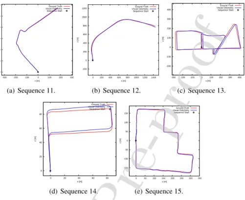
0 100 200 300 400 500 600 -300 -200 -100 0 100 200 300 z [m] x [m] Ground Truth Visual Odometry Sequence Start (a) Sequence 11. -200 0 200 400 600 800 1000 1200 0 200 400 600 800 1000 1200 1400 z [m] x [m] Ground Truth Visual Odometry Sequence Start (b) Sequence 12. -200 -100 0 100 200 300 400 -300 -200 -100 0 100 200 300 400 z [m] x [m] Ground Truth Visual Odometry Sequence Start (c) Sequence 13. 0 20 40 60 80 0 20 40 60 80 z [m] x [m] Ground Truth Visual Odometry Sequence Start (d) Sequence 14. -150 -100 -50 0 50 100 150 0 50 100 150 200 250 300 350 z [m] x [m] Ground Truth Visual Odometry Sequence Start (e) Sequence 15.
Figure 8: The predicted trajectories of LKN on the sequences 11-21 from the KITTI dataset. The learning model is trained on the sequences 00-10. Please note the results of sequences 16-21 are not provided on the official website.
8. Appendixes
8.1. Appendix A: Online Submission Evaluation on KITTI Dataset
The evaluation on sequences 11-21 for the model trained on sequences 00-10 is performed using the online submission portal of the KITTI dataset. The quali-tative and quantiquali-tative results are shown in Figs. 8 and 9. The LKN VO achieves
an overall performance of2.66%for average translational error and0.79◦/100m
for average rotational error on sequences 11-21 from the KITTI dataset. Please note the results of sequences 16-21 are not provided on the official website. More
detail can be found on our online KITTI submission website13.
13http://www.cvlibs.net/datasets/kitti/eval_odometry_detail.
php?&result=e2b9434f9bd33770c66680871e8262990d0a780a
Journal
Pre-pro
of
0 0.5 1 1.5 2 2.5 3 3.5 100 200 300 400 500 600 700 800 Translation Error [%] Path Length [m] Translation Error
(a) Translation vs Path Length.
0 0.002 0.004 0.006 0.008 0.01 0.012 0.014 100 200 300 400 500 600 700 800
Rotation Error [deg/m]
Path Length [m]
Rotation Error
(b) Rotation vs Path Length.
0 1 2 3 4 5 6 7 10 20 30 40 50 60 70 80 90 Translation Error [%] Speed [km/h] Translation Error (c) Translation vs Speed. 0 0.002 0.004 0.006 0.008 0.01 0.012 0.014 0.016 10 20 30 40 50 60 70 80 90
Rotation Error [deg/m]
Speed [km/h]
Rotation Error
(d) Rotation vs Speed.
Figure 9: Average translational and rotational errors of LKN against different path lengths and speeds. The learning model is trained on sequences 00-10 and evaluated on sequences 11-21.
8.2. Appendix B: Qualitative Results on Apolloscape Dataset
Some selected qualitative results of LKN on Apolloscape Dataset are shown in Fig. 10.
8.3. Appendix C: Network Architecture
Figs. 11 and 12 show the operations and parameters of the observation, tran-sition and LSTM prior networks in LKN deployed on KITTI and Apolloscape datasets correspondingly.
Journal
Pre-pro
of
X(m) -150 -100 -50 0 50 100 150 200 250 Y(m) -300 -250 -200 -150 -100 -50 0 GT LKN
(a) Road11, Record010.
X(m) -550 -500 -450 -400 -350 -300 -250 -200 -150 Y(m) -300 -250 -200 -150 -100 -50 0 GTLKN (b) Road11, Record011. X(m) -500 -450 -400 -350 -300 -250 -200 -150 Y(m) 240 260 280 300 320 340 360 380 400 420 GT LKN (c) Road11, Record031. X(m) 100 200 300 400 500 600 Y(m) 440 460 480 500 520 540 560 580 600 620 GT LKN (d) Road12, Record008. X(m) -200 -150 -100 -50 0 50 100 150 Y(m) 600 650 700 750 800 850 900 GT LKN
(e) Road12, Record009.
X(m) 50 100 150 200 250 300 350 400 Y(m) 1180 1200 1220 1240 1260 1280 1300 1320 1340 1360 1380 GT LKN (f) Road12, Record034. X(m) -200 -180 -160 -140 -120 -100 -80 -60 -40 Y(m) 720 740 760 780 800 820 840 860 880 900 GT LKN (g) Road12, Record036. X(m) 1050 1100 1150 1200 1250 1300 Y(m) -300 -200 -100 0 100 200 300 GT LKN (h) Road14, Record018. X(m) 600 700 800 900 1000 1100 1200 Y(m) 350 400 450 500 550 600 650 700 GT LKN
(i) Road16, Record009. Figure 10: The predicted trajectories of LKN on the Apolloscape dataset. The training and test sequences are split as shown in Table 3.
Journal
Pre-pro
of
Figure 11: The detailed architecture and parameters of the observation, transition and LSTM prior networks in LKN deployed on the KITTI dataset.
Journal
Pre-pro
of
Figure 12: The detailed architecture and parameters of the observation, transition and LSTM prior networks of LKN deployed on the Apolloscape dataset.
Journal
Pre-pro
of
Journal
Pre-pro
of
LI SUN received the PhD from University of Glasgow in 2016. Now he is a post-doctoral research fellow with Oxford Robotics Institute, University of Oxford. He is IEEE, BMVA, EUcog, SICSA member. From 2017 to 2018, he was a research associate with the Lincoln Centre for Autonomous Systems, University of Lincoln, UK. Before that, he was working as a research fellow at Extreme Robotics Lab, University of Birmingham, UK. Dr. Li Sun’s research focuses on the core challenges in the emerging robot vision to enable the robot to manipulate with complex industrial objects or drive in the dynamic, real-life environment e.g. warehouse, urban driving.
Journal
Pre-pro
of
Zhi Yan is currently an Assistant Professor in the Distributed Artificial Intelligence and Knowledge Laboratory (CIAD) at the University of Technology of Belfort-Montbéliard (UTBM). From 2016 to 2017, he was a Postdoctoral Research Fellow in the Lincoln Centre for Autonomous Systems (L-CAS) at the University of Lincoln, working on the Horizon 2020 project FLOBOT. From 2013 to 2015, he was a Postdoctoral Research Fellow in the CAR Team at the IMT Lille Douai. In 2012, he received his Ph.D. from the Paris 8 University. His research interests are in autonomous driving, mobile robotics, and chronorobotics.
Journal
Pre-pro
of
Gerhard Neumann is a Professor of Robotics and Autonomous Systems with the University of Lincoln, Lincoln, U.K.. Before coming to Lincoln, he has been an assistant professor at the TU Darmstadt from September 2014 to October 2016 and head of the Computational Learning for Autonomous Systems (CLAS) group. Before that, he was Post-Doc and Group Leader at the Intelligent Autonomous Systems Group (IAS) also in Darmstadt under the guidance of Prof. Jan Peters. Gerhard obtained his Ph.D. degree under the supervision of Prof. Wolfgang Mass at the Graz University of Technology. He is principle investigator for the National Center for Nuclear Robotics (NCNR) in Lincoln which is an EPSRC RAI Hub and also leading 1 Innovate UK project on Tomato Picking. In Darmstadt, he is principal investigator of EU H2020 project Romans and also already acquired DFG funding.
Journal
Pre-pro
of
Tom Duckett is a Professor of robotics & autonomous systems with the University of Lincoln, Lincoln, U.K., where he also leads the Lincoln Centre for Autonomous Systems. His research interests include autonomous robots, artificial intelligence, machine perception, and robotic mapping, with applications including agri-food and service robotics. He has been an investigator in many national and international research projects, funded by the European Commission, the U.K. Research Councils and Innovate U.K., including ILIAD, STRANDS, and various projects in precision agriculture. He worked previously at the Centre for Applied Autonomous Sensor Systems, Örebro University, Sweden, where he led the Learning Systems Laboratory. He obtained his PhD in the AI Group at the University of Manchester, UK. Prior to becoming an academic, he worked for several years as a programmer, developing and supporting software solutions for the fresh food industry.
Journal
Pre-pro
of
Rustam Stolkin received the M.Eng. degree in engineering science from the University of Oxford, Oxford, U.K., in 1998, and the Ph.D. degree in computer vision from University College London, London, U.K., in 2004. He is a Royal Society Industry Fellow. He is currently the Director of U.K.’s National Centre for Nuclear Robotics and a Professor of robotics with the University of Birmingham, Birmingham, U.K., where he is the Founder and Director of the Extreme Robotics Lab. He is also the Director of spinout company A.R.M Robotics Ltd. His research interests include computer vision and image processing, machine learning and AI, vision-guided robotic manipulation, and human-robot interaction.
![Table 1: The comparison of performance of LKN against the baselines on the KITTI dataset according to the evaluation method [10]](https://thumb-us.123doks.com/thumbv2/123dok_us/1293524.2673403/18.892.160.733.827.960/table-comparison-performance-baselines-kitti-dataset-according-evaluation.webp)