ISSN: 2394-3661, Volume-4, Issue-6, June 2017
Abstract— This research is focused on the consistent, robust least squares dummy variable (LSDVR) estimator which is predicated on the correction of the bias of the inconsistency of the least squares dummy variable estimator of the parameters of the dynamic panel data model, as an extension of earlier results. We compared the results of the bias corrected least squares dummy variable estimator of the dynamic panel data models in the presence of outliers, at stated specifications of the model with the consistent instrumental variable (IV) and the generalized method of moments (GMM) estimators of Anderson and Hsiao (AH), Arellano and Bond (AB) and Blundell and Bond (BB) to validate the claims or otherwise of the estimators. We observe at =
=0.8 and B=0.2 that the robust least squares dummy variable estimator (LSDVR) performs better than the IV- GMM in finite and large samples in terms of predictive powers and in the estimation of the autoregressive coefficient in large samples followed by the LSDV, though, with maximum RMSE property while the Blundell and Bond (BB) performs better than the other contending models in estimation of the autoregressive coefficient in finite samples showing that the presence of an outlier does not affect the predictive power of the robust least squares dummy variable (LSDVR) estimator.Index Terms— Consistent estimator, dynamic, outliers, panel data model
I. INTRODUCTION
Leveraging on the exposition by [1] that the Least Squares dummy variable estimator is inconsistent in determining the estimates of the parameters of a first order autoregressive panel data model at finite time period, T, as the cross sectional units, N, becomes infinitely large, certain instrumental variable (IV) and generalized method of moments (GMM) estimators have been proposed in the econometric literature in the accounts of [2], [3] and [4].
However, the IV-GMM estimators which includes the Anderson Hsiao (AH) instrumental variable estimators, Arellano and Bond (AB) generalized method of moments estimators and Blundell and Bond (BB) system generalized method of moments estimator Could not provide all the cure for all the problems inherent in the model as a result of the violation of assumption of absence of correlation between the explanatory variable and the error term: a condition upon which the ordinary least squares and hence the least squares dummy variable estimator could be both consistent and efficient. In the accounts of [5], [6], [7], [8] and [9], the
Okeke Joseph Uchenna, Department of Mathematics and Statistics, Federal University Wukari, Wukari, Nigeria, +2348036026806
Okeke Evelyn Nkiruka, Department of Mathematics and Statistics, Federal University Wukari, Wukari, Nigeria, +2348142671318
Obi Jude Chukwura, Department of Statistics, Chukwuemeka Odumegu Ojukwu University, Uli, Nigeria, +2348037474454
system GMM was proposed as a result of the weakness of the first-differenced instrumental variable IV-GMM estimators which suffered small sample bias due to weak instruments. In clear terms, all the IV-GMM estimators maintained their consistency property, with highly persistent data, when the cross section units, N, is large but could be severely biased in small samples as in [5]. In large samples, the LSDV estimator, though inconsistent, has a small variance, relatively compared to the IV-GMM methods as observed by [1], [10] and [11]. The fact that the LSDV may be consistent in large samples in the direction of T is buttressed by [5] and [7], but has higher variance relative to the IV-GMM estimators in small samples with highly persistent data says [12].
Also , in highly persistent data, the Bias corrected least squares dummy variable (LSDVR) estimation of a first order autoregressive Panel data model which involves the approximation of the bias of the least squares dummy variable estimator and taking care of the bias to produce an estimator that could be consistent both in large and small samples emerged in the accounts of[1],[13] and [7].
[1] and [13] used higher order asymptotic expansion approximation techniques of order N-1T-1 and N-1T-2 respectively to obtain the small sample bias of the LSDV under the assumption of homoscedasticity.[14] obtained the bias corrected LSDV estimator for a case of cross section units heteroscadasticity. [7] obtained the bias corrected least squares dummy variable estimator for samples under the assumption of homoscedasticity and also worked on the bias correction model of the LSDV in the case of time series and cross section heteroscedasticity, an extension of the work by [14].
This paper is a further extension of the work of [14] and [7] and deals strictly with the comparison of the performances of the LSDV,LSDVR, AH, AB and BB estimators in the presence of an outlier. An effort, still, in search of supportive evidence of their performances in the first order autoregressive panel data model that is still evolving.
A. Weak Instrument
An instrumental variable is a proxy which is highly correlated with the included endogenous variable in the dynamic panel data model but uncorrelated with the error term. The strength of the correlation can be determined using the F-statistics since the instrument and instrumented are observable.
In the first order autoregressive panel data model given by
y
it
y
it1
X
it'
V
it whereV
it
αi+εitRobust Least Squares Dummy Variable Estimation
Of Dynamic Panel Models In The Presence Of
Outliers
test to determine the absence of correlation between the instrument and the error term is conducted using the Sagan-Hansen test statistic calculated as
TR
2.R
2 is the coefficient of multiple determination obtained from the OLS residuals onto the exogenous variable and T is period as in [4]. In a system of linear models, the test is not feasible in exactly identified model but rather in over identified models where it is expected that the instruments are truly exogenous and uncorrelated with the error term says [15].The presence of instruments that are correlated with the error term or that are poorly correlated to the endogenous explanatory variable can make the estimates obtained to be inconsistent and are thus regarded as weak instruments. A weak instrument produced wrong estimates of parameters and standard errors while the good instrument is expected to be highly correlated with the instrumented and uncorrelated with the error to produce correct estimates of the parameters and their standard errors.B. Generalized Method of Moments (GMM) Estimator
Generalized method of moments (GMM) estimation is the application of Instrumental variable to an over-identified model, i.e. when the number of instruments is greater than or equal to the number of covariates in the equation of interest. It should be recalled that if instruments are greater than the number of covariates, this is over identification. In other words, the GMM is a generalization of the just-identified instrumental variable estimator.
The danger of instrumental variable method is that it may be difficult to find a good instrument but may introduce multicollinearity. Hence [4] and [5] suggested the use of maximum likelihood estimation method with it limitations: methodologically and practical wise, especially in data involving large cross sections.
C.Heteroscedasticity
Heteroscedasticity is the presence of unequal variance of the error term in a model. Unequal error variance is a violation of the assumption of equal error variance (homoscedasticity) upon which the OLS is BLUE and efficient which is worth correcting only when it is severe as in [4]. However, in the presence of heteroscedasticity OLS is BLUE but not efficient. Under heteroscedasticity the estimates of the coefficients using OLS is unbiased but their standard errors may be biased in the accounts of [4] and [16].
D.Outlier
An outlier is an observation, which is much different in magnitude, i.e. either very large or very small compared to other observation within the same sample. In other words, they are perceived to be from a population other than that from which the other sample observations are generated as in [4] and [15]. Outliers could be a source of heteroscedasticity. Outliers could be a result of the unobservable individual effects in a panel data study, such as effects of government policies, available resources and their uses, political will of the leader, level of patriotism of the citizenry, and generally, the individual attributes of the units of a cross-section.
II. APPROXIMATING THE INCONSISTENCY OF THE LSDV
y
it
y
it1
X
it'
i
it, I=1,2,…,N; t=1,2,…,T (1)where
y
itis the value of y for the ith individual or group at period, t, a TX1 vector of dependent variable.y
i,t1is the immediate value of y at the immediate past one period t-1 for the ith cross section unit or group.X
itis the value of the exogenous explanatory variable at period, t for the ith cross section unit or group and ((N-1) X1) vector .
i is the unobserved ith unit or group effect term and
itis an error term that has mean zero and variance
2.When we consider the LSDV by within estimation obtained by the application of the ordinary least squares on the transformed model:
y
~
~
y
1
X
~
~
(2) such that:
ˆ
(
w
~
'w
~
)
1w
~
'y
(3) and:w
~
[
~
y
1,
X
]
(4) 1~
y
andX
~
are observations that have been centered and stacked over time such that~
y
1 is an (NTX1) vector of lagged endogenous explanatory variable andX
~
is an (NTX1) vector of strictly exogenous explanatory variables in the accounts of [7].
ˆ
(
,
')
(5)
ˆ
is an ((N+1)X1) vector of coefficients as in [5].The inconsistency of the LSDV at finite period, T and large cross section units,N, is evidenced by
cov[(
y
~
it1
y
i,1)(
~
it
)]
o
(6) and can be estimated using partition regression technique in line with [7],for the errors of
and
as
ˆ
(
y
~
'1D
~
y
1)
1y
'1
~
(7)
ˆ
(
~
~
)
~
~
(
ˆ
)
(
~
'ˆ
)
1~
'~
1 ' 1 'X
X
y
X
X
X
(8) where:
~
~
y
w
~
ˆ
(9) andD
1
X
~
(
X
~
'X
~
)
1X
~
'.Then taking probability limits, we have:
) ~ ~ 1 lim ( ) ~ ~ 1 lim ( ) ˆ ( lim '1 1 y'D N P y D y N P P N N N (10)
lim (ˆ) lim (~'~)1~'~1 lim (ˆ)
N N N P X X X y P P (11)
From (10): lim 1 ~ ~ lim 1 ~' ~
1 ' 1 y N P D y N P N N (12) because X is assumed to be strictly exogenous.
Then from (12) ]) ~ ~ [ ( 1 ~ ~ 1 lim '1 ' 1
E y N y N PLim
N N (13)ISSN: 2394-3661, Volume-4, Issue-6, June 2017 By further decomposition, we obtain
(
~
'~
)
(
)
1
tr
T Ty
E
(14) Substituting (14) into (13), we obtain (15) in accordance with [7] and [14].) ( ) 1 ( ) ( 1 ~ ~ 1 lim 1 ' 1 T T N i i N T T T N N tr N Lim tr tr N Lim y N P
(15) Under the assumption of homoscedasticity for whichT T
I
2
, we have that ) ) 1 ( 1 1 1 ( ) ( ) ( ~ ~ 1 lim 2 2 2 2 ' 1 T tr I tr y N P T T T T N (16) which would result to the bias approximations below with reasonable level of accuracy:) ( ); ( ); ( 1 2 3 2 3 1 1 2 1 2 1 1 1 c T B B c N T B B c N T B (17) where
c
1,
c
2andc
3depended on the unknown parameters2
and
.Substituting (15) into (10) we obtain:
P
lim
N(
ˆ
)
tr
(
T
T)
/
2y1/X (18) Also, substituting (14) into (9), we obtain)
ˆ
(
lim
)
ˆ
(
lim
N
P
N
P
(19) (18) and (19) are the bias approximation of the LSDV estimator derived by [7] directly from the data without initial resort to any consistent estimator1 '
~
~
1
lim
1
X
y
N
P
N xy ,X
X
N
P
N xx~
~
1
lim
'
and
y21/X
(
1
xy21)
y21. 1 1 1 1 1 ' 2
xy xy xy xy
is the squared multilple correlationcoefficient of
y
1 regressed on X and 11
xy xx
is thecorresponding vector of regression coefficients for
and
unknown.III. ROBUST LEAST SQUARES DUMMY VARIABLE (LSDVR) ESTIMATOR
The robust least squares dummy variable estimation is predicated on the derivation of an approximate expression for the inconsistency of the LSDV which could be used to correct for the bias of the LSDV. In [5], the robust LSDV estimator is implemented by finding consistent estimates for
2 and
, subtracting each or any of the bias approximationB
cin (17) from the LSDV obtained by within estimation, we obtain the robust LSDV,LSDV
R, estimator below:
LSDV
R
LSDV
B
ˆ
c, c= 1, 2 and 3: AH=1, AB=2 and BB=3 (20) The consistent estimator of
2 is obtained by' 2
ˆ
c c ce De
N
K
T
,N
T
K
(21) wheree
c
y
w
H
ˆ
cand C= AH, AB and BB, are the consistent estimators of
.It is pertinent to point out, at this juncture, that the bias approximation derived by [1], [2] and [7] assumed homoscedasticity of the error variance in their studies. The additive bias corrected LSDV estimator by [7] , just like that of [2], relied upon the consistent IV-GMM estimators of
to determine the bias such that the bias corrected LSDV estimators are: 2 / . . 1)
ˆ
ˆ
(
ˆ
ˆ
X y gmm T Gmm T DVtr
(22) 1 . . 2 /ˆ
ˆ
(
)
ˆ
ˆ
T Gmm T Gmm DV y Xtr
(23)where
T.GMM and
T.GMM are the variance structures which depended on
and
respectively, and can be obtained by their sample equivalence as explained earlier in a section above while
T can be estimated from:
ˆ
T.GMM
diag
(
ˆ
t2.gmm)
(24) For which ' 1 1 2 .ˆ
ˆ
ˆ
ˆ
(
) (
)
ˆ
(
1) /
t gmm t t gmm gmm t t gmm t gmmy
y
X
y
y
X
N T
T
(25)and
~
y
t,
~
y
t1andX
~
tare stacked across individuals such that)
~
,...,
~
,
~
(
~
2 1t t Nt ty
y
y
y
According to [7] , to take care of a non linear bias correction, the bias corrected estimator is not feasible for
is obtained by solving 2 1/(
)
ˆ
T T y Xtr
for
while assuming,first, that the variance structure
Tis given by
y21and
. T
, 21
y
and
are all unknown and the consistent estimator of
T [7].By a system of K equations, the bias corrected
and
are obtained from 2 / 1ˆ
)
ˆ
ˆ
(
ˆ
DV
tr
T
T
y X
(26) 1 2 /ˆ ˆ
ˆ
(
)
ˆ
DVtr
T T y X
(27) where
ˆ
T
diag
(
ˆ
t2)
;T
T
N
X
y
y
X
y
y
t t t t t t/
)
1
(
)
~
~
~
(
)
~
~
~
(
ˆ
1 ' ' 1 2
IV. DESIGN OF THE EXPERIMENT
To provide for effective comparison of the performance of the robust LSDV estimator, (
LSDV
R), against the AH, AB, andBB, we generated the
y
tvalue as it is defined in (1), i.e. Yit =X1it +
Yit-1 + i + εit , a simple dynamic panel data modelwith fixed effects i.e. having a time invariant individual or group specific effects, i , and generated
X
t using the generating equation Xit = Xit-1 + et , eN(O,1), / /<1,making provision for an outlier.
We specified =0.8,
=0.8 and =0.2 in the general models and specified two models: (1) for finite samples (i.e. n=11 and t=50) and (2) for large samples (i.e. n=51 and t=10). The start up values Yi0 and Xi0 are obtained using theprocedures by [17]. for i = Q1 it+ , , we fix Q1
at 0.8 as in [18]. We then used the within estimation of (2) to obtain the LSDV parameter estimators which are and . The experiment conducted is replicated five hundred (500) times. The root mean square errors (RMSE) of the estimated model, the root mean square errors (RMSE
) of the estimated autoregressive coefficients as well as the Akaike Information Criterion (AIC) are employed for model comparisons. We employed Stata 10.0, Excel 2007 and Minitab statistical packages in the analysis to cushion the cumbersome nature of some estimators,V. RESULTS AND DISCUSSIONS
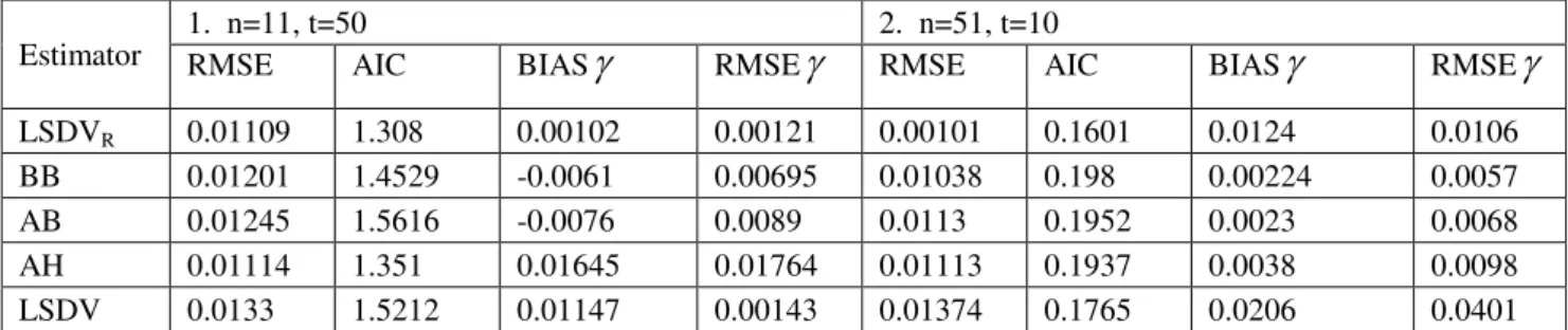
The results of the simulation analysis for the various estimators considered is shown in the table 1 below at the two specifications of time and cross-sections for =
=0.8 and =0.2.Table 1. Simulation analysis of the various estimators of the dynamic panel data model in the presence of outliers Estimator
1. n=11, t=50 2. n=51, t=10
RMSE AIC BIAS
RMSE
RMSE AIC BIAS
RMSE
LSDVR 0.01109 1.308 0.00102 0.00121 0.00101 0.1601 0.0124 0.0106
BB 0.01201 1.4529 -0.0061 0.00695 0.01038 0.198 0.00224 0.0057
AB 0.01245 1.5616 -0.0076 0.0089 0.0113 0.1952 0.0023 0.0068
AH 0.01114 1.351 0.01645 0.01764 0.01113 0.1937 0.0038 0.0098
LSDV 0.0133 1.5212 0.01147 0.00143 0.01374 0.1765 0.0206 0.0401
From the results of the study, the Blundell and Bond (BB) generalized method of moments (gmm) consistent estimator recorded minimum error in the autoregressive term with RMSEY=0.0057 in finite samples with large number of cross-sections (n=51) and finite period of time (t=10) or specification 1: this buttressed the results of [2], [7], [12] and [5], while the robust least squares dummy variable estimator (LSDVR) showed high predictive power of the model by returning the least values in the RMSE=0.0010 and AIC=0.1601 at the same specification 2 as well as in specification 1. The robust least squares dummy variable estimator (LSDVR) recorded the minimum error values of the autoregressive term with RMSEY=0.00121 in specification 1. The error values are generally lower in specification 2, relatively, compared to those of the specification 1. The unsteady nature of the Arellano and Bond (AB) consistent estimator that led to the introduction of the BB system GMM estimator is seen as it recorded higher values of RMSE’s of 0.01245 and 0.0113 in specifications 1 and 2 respectively, relative to the other consistent estimators. However, the LSDVR recorded minimum RMSEY of 0.00101 in finite samples with large cross-section of n=51 and t=10 which is in agreement with the report of [7]. The bias of the least squares dummy variable estimator is approximated by the Blundell and Bond (BB) and its effects on the results of the robust least squares dummy variable estimator is quite glaring as the robust least squares dummy variable estimator (LSDVR) produced the minimum error in large samples of small number of cross sections (n=11) and long time period (t=50). It is observed that even in the presence of outliers the
predictive power of the robust least squares dummy variable estimator (LSDVR) is more powerful than the other competing models and it is the most efficient except in the finite sample where the BB is the most efficient model in estimating the autoregressive coefficient.
ACKNOWLEDGMENT
We sincerely appreciate the authors whose works are cited in this research paper for their thought evoking works that made us to seek solution that may validate some claims of the dynamic panel model estimators.
REFERENCES
[1] S. Nickel, “Biases in dynamic models with fixed effects,” Econometrica, Vol. 49, 1981, pp.1417-1420.
[2] J. F. Kiviet. “On bias, inconsistency and efficiency of various estimators in dynamics panel data models,” Journal of Econometrics, Vol. 68, 1995, pp. 53-78.
[3] M.R. Abonazel. “Bias correction methods for panel data
models with fixed effects. Mj Journal on Statistics and Probability. Vol.1, 2016. pp 37-51.
[4] D.N. Gujarati, Basic of Econometrics, fourth Ed. New York, Tata McGraw-Hill, 2003, pp. 636-719.
[5] G.S.F. Bruno, “Estimation, inference and Monte Carlo analysis in dynamic panel data models with a small number of individuals,” The Stata Journal, Vol. 5, No.4, 2004, pp. 473-500.
[6] G.S.F. Bruno, “Approximating the bias of the LSDV estimator for dynamic unbalanced panel data models,” Economics Letters, vol.87, 2005, pp. 261-266.
[7] M.G.J. Bun, and M. A. Carree, “Bias-corrected estimation in dynamic panel data models,” Journal of Business and Economic Statistics, vol.23, 2005, pp. 200-210.
ISSN: 2394-3661, Volume-4, Issue-6, June 2017
[8] J.U. Okeke, J. C. Nwabueze, and E. N. Okeke , “Robust regression models of dynamic panel data,” International Journal of Scientific Research, DOI: 10.15373/22778179, vol.4, No.10, 2015, pp. 198-201. Available @ http://www.ijsr.org.
[9] B.H. Baltagi, Econometric Analysis of Panel Data, 5th ed. Chichester, John Wiley and Sons, 2013.
[10] R.A. Judson, and A. L. Owen, “Estimating dynamic panel data model: a guide for Macroeconomists,” Economics Letters, vol.65, 1999, pp. 9-15.
[11] J.F. Kiviet, “Judging contending estimation by simulation: tournaments in dynamic panel data models,” Tinbergen Institute Discussion paper, University of Amsterdam, 2005.
[12] M. Bun, and J. Kiviet, “On the diminishing returns of higher order terms in asymptotic expansion of bia,” Economics Letters, vol.79, 2003, pp.145-152.
[13] J. U. Okeke, and E. N. Okeke, “Least squares dummy variable in determination of dynamic panel model parameters,” European Journal of Engineering Research and Science, vol.1, No. 6, 2016, pp. 77-80Available@ http:// www.ejers.org.
[14] P.C.B. Phillips, and D. Sul, “Bias in dynamic panel estimation with fixed effects,incidental trends and cross section dependence,” Cowles Foundation Discussion Paper. No.1438, Yale University, 2004.
[15] W.H. Greene, Econometric Analysis, 4th ed, Engle-Wood Cliffs, Prentice Hall, 2003.
[16] A. Koutsoyiannis, Theory of Econometrics, 2nd ed, New York, Palmgrove Publishers Ltd, 2001.
[17] A.I. McLeod, and K.W. Hipel, “Simulation procedure for Box-Jenkins
models,” Water Resources Research, vol.14, 1978, pp. 969-975.
[18] J.U. Okeke, E.N. Okeke, and J.C. Nwabueze, “Individual effects on stable first order autoregressive panel data models,” International Journal of Science: Basic and Applied Research, ISSN 2307 4531, vol.19, no.1, 2015, pp. 279-284. Available @ http:// www.ijsbar.org.
Okeke, Joseph Uchenna was born in Asaba, Delta State, Nigeria , on the 14th May, 1971. He holds: PhD Statistics (2011) from ABSU, Abia, Nigeria; M.Sc. Statistics (2005) from NAU, Anambra, Nigeria and B.Sc. Statistics (1997) also from NAU. His major field of study is Econometric statistics with stint in multivariate statistics which was his area of research at his masters thesis.
He was a LECTURER at the Anambra State University now Chukwuemeka Odumegwu Ojukwu University (2007-2013). Presently, he lectures in the Department of Mathematics and Statistics of the Federal University Wukari, Taraba State, Nigeria. He has published in both local and foreign reputable journals. His research interests are in the areas of Econometric modeling and Multivariate modeling.
Dr. Okeke is a member of the Nigerian Statistical Association, a consultant with the United Nations Development Program, the Secretary, Anambra West Elite Club (2012 to date), the seminar coordinator, Faculty of Pure and Applied Sciences, Federal University Wukari, Nigeria. Okeke, Evelyn Nkiruka was born in Obeledu, Anambra State, Nigeria, on the 16th July, 1971. She holds: PhD Statistics (2011) from ABSU, Abia, Nigeria; M.Sc. Statistics (2002) from NAU, Anambra, Nigeria and B.Sc. Statistics (1997) from NAU, Anambra , Nigeria. Her major field of study is Multivariate statistics(Discrimination and classification) and also has interest in Econometric modeling.
She was a LECTURER at the Nnamdi Azikiwe University (NAU, Awka) 2001-2013. Presently, she lectures in the Department of Mathematics and Statistics of the Federal University Wukari, Taraba State, Nigeria. She has published in both local and foreign reputable journals. Her research interests is in the area of Discriminant Analysis.
Dr.Mrs. Okeke is a member of the Nigerian Statistical Association, a consultant with the United Nations Development Program, the Head, Department of Mathematics and Statistics, Federal University Wukari, Nigeria. Chairperson Welfare committee, Faculty of Pure and Applied Sciences, Federal University Wukari, Nigeria.
Obi, Jude Chukwurah was born in Awkuzu, Anambra State, Nigeria , on the 21th June, 1968. He holds: PhD Statistics (2017) from University of Leeds, UK; M.Sc. Statistics (2005) from NAU, Anambra, Nigeria and B.Sc. Statistics (1997) also from NAU. His major field of study is Computational Statistics with base in multivariate statistics which was his area of research at his masters thesis.
He is a LECTURER at the Chukwuemeka Odumegwu Ojukwu University (2006 till date). He has published in both local and foreign reputable journals. His research interests are in the areas of Econometric modeling and Multivariate modeling.