Convolutional Support Vector Machines For Image Classification

(1)

Convolutional Support Vector Machines For Image

Classification

Benjamin Sugg

Submitted by Benjamin Sugg to the University of Exeter as a thesis for the degree of Masters by Research in Computer Science, May 2018.

This thesis is available for Library use on the understanding that it is copyright material and that no quotation from the thesis may be published without proper acknowledgement. I certify that all material in this thesis which is not my own work has been identified and that

any material that has previously been submitted and approved for the award of a degree by this or any other University has been acknowledged.

(2)

The Convolutional Neural Network (CNN) is a machine learning model which excels in tasks that exhibit spatially local correlation of features, for example, image classification. However, as a model, it is susceptible to the issues caused by local minima, largely due to the fully-connected neural network which is typically used in the final layers for classification. This work investi-gates the effect of replacing the fully-connected neural network with a Support Vector Machine (SVM). It names the resulting model the Convolutional Support Vector Machine (CSVM) and proposes two methods for training. The first method uses a linear SVM and it is described in the primal. The second method can be used to learn a SVM with a non-linear kernel by casting the optimisation as a Multiple Kernel Learning problem. Both methods learn the convolutional filter weights in conjunction with the SVM parameters. The linear CSVM (L-CSVM) and kernelised CSVM (K-CSVM) in this work each use a single convolutional filter, however, approaches are described which may be used to extend the K-CSVM with multiple filters per layer and with multiple convolutional layers. The L-CSVM and K-CSVM show promising results on the MNIST and CIFAR-10 benchmark datasets.

(5)

Chapter 1

Introduction

1.1 Motivation

The Support Vector Machine (SVM) (Boser et al., 1992) is an influential machine learning model which has been successfully applied to a broad range of learning tasks. It is an attractive model to researchers due to the fact that it may be trained by optimising a convex error function. Thus, training is guaranteed to find parameters which achieve a globally optimum solution and the same solution will be found each time that the model is trained with the same data.

However, in recent times, the popularity of the SVM has declined in favour of deep learning models. These are models which are characterised by the presence of many processing nodes assembled into a stacked topology. Classification is a black-box procedure for deep learning models as the abundance of nodes makes the internal workings difficult to comprehend. A subclass of deep learning model which has had notable success in the image recognition domain is the Convolutional Neural Network (CNN) (LeCun et al., 1989). The key to the CNN’s success is the inclusion of sparsely connected layers named convolutional layers. These allow the model to extract spatial information from its inputs which is unavailable to many other models. The convolutional layers act as feature extractors before an input is passed to a neural network for prediction. The CNN has achieved state-of-the-art results on many benchmark datasets, for example, MNIST (LeCun et al., 1998a), ImageNet Large Scale Visual Recognition Challenge (Russakovsky et al., 2015) and Caltech 256 (Griffin et al., 2007).

Despite its success, the CNN, along with many other forms of deep learning, faces difficulties during training due to the irregularity of its error landscape. The large number of connection weights which are involved make it particularly susceptible to the complications caused by local minima. This work explores the idea of replacing the fully connected neural network, which a CNN typically uses for prediction, with a SVM. Thus the convolutional layers may be considered feature extractors before prediction using a SVM. The aim of this is to create a hybrid classifier which is able to utilise the spatial information of its input values while retaining the convex properties of SVM optimisation.

(6)

1.2 Contributions

The principle contributions of this thesis are two algorithms, named the L-CSVM and K-CSVM algorithms, for training the Convolutional SVM hybrid classifier.

The L-CSVM algorithm, described in Algorithm 4, is an iterative, two-step optimisation which may be used to learn a linear SVM with a convolutional feature extractor. It first learns the SVM primal weight vector by fixing the filter coefficients, then it learns the filter coefficients by fixing the weight vector. These steps are repeated until convergence. The novel aspect of the algorithm is the fact that it casts the filter update step as a SVM training problem. By doing this, the filter may be learned using an arbitrary SVM training algorithm. Thus, both of the training steps are convex with respect to the parameters.

The K-CSVM algorithm, presented in Algorithm 5, may be used to learn a kernelised SVM with a convolutional feature extractor. It does this by formulating the optimisation problem as a Multiple Kernel Learning (MKL) optimisation problem. The K-CSVM algorithm is based on the GMKL algorithm, proposed in (Varma and Babu, 2009), but it has been adapted for filter learning. To this authors knowledge, this is the first research in which convolution has been integrated into a kernelised SVM.

1.3 Thesis Organisation

The thesis continues in chapter 2 by providing background to the image recognition domain. The aim of the chapter is to establish notation and to provide the prerequisite information required to understand the concepts proposed in chapters 3 and 4. Chapter 3 presents the Linear Convolutional SVM. It provides details of previous research in this domain and then proposes a training algorithm. The algorithm is tested and analysed using the MNIST dataset. Chapter 4, titled Kernelised Convolutional SVMs, explores how a convolutional filter may be used to augment a kernelised SVM. It presents an algorithm for training and tests the model on the MNIST and CIFAR-10 datasets. The thesis is concluded in chapter 5.

(7)

Chapter 2

Background

This chapter begins with a description of supervised learning in section 2.1; the description is model agnostic, with the intention of establishing notation. Section 2.2 introduces the first model for supervised learning: the Linear Perceptron. Section 2.3 shows how the Linear Perceptron may be extended to learn a non-linear hyperplane by introducing the Multi-layer Perceptron. This is further adapted in section 2.4 where it is explained how convolution may be used to specialise the Multi-layer Perceptron for image recognition. Section 2.5 describes an alternative model for supervised learning named the Support Vector Machine. It shows how the primal formulation of a Support Vector Machine may be used to learn a linear hyperplane and then explains how a kernel function may be employed in the dual in order to learn a non-linear hyperplane. Section 2.6 completes the background with a description of Multiple Kernel Learning.

2.1 Supervised Learning

The high-level aim of supervised learning is to obtain a function which can take a set of properties and map them to a target output. The properties, named features, are collated into a vector,

x∈RM, and the target output,y, may be a real value or a class label. The tuple(x, y)forms an instance of some learning problem. The mapping function, denotedf, requires a configuration,

θ, which determines the importance of items inx for approximatingy. Thus f : (x,θ)7→y. It is the job of a supervised learner to tuneθ using data for which the mappingx7→y is already known. This process is named training and it will be described in more detail as this chapter progresses. Once training has been used to obtain a suitableθ,fmay be used to make predictions about data for whichy is unknown. The estimation is denotedyˆand it is not necessarily equal toy. Thus:

ˆ

y=f(x,θ). (2.1)

As an example of supervised learning, consider a town containingNhouses. Three properties are known about each house: the floor space measured in square feet, the total number of floors and the number of bathrooms. Thus eachxncontains three elements wherenranges between1 andN+ 1. In this case,M = 3. The market value of some of the houses is known, but it is not

(8)

known for all. This acts as the target valueyn. In this scenario, the task of a supervised learner

may be to find a relationship between the properties of a house and its market value, so that the houses without a known market value can be estimated.

To tune θ, a supervised learner examines a training dataset. This is a set where the true target is known for each of the instances. The training dataset is denotedDand may be defined as:

D={(xn, yn)}Nn=1. (2.2)

Learning is achieved by finding a θ which minimises the overall difference between y and yˆfor each of the instances in the training dataset. To measure the difference, a loss function `(y,yˆ)

is used. The choice of` depends on the type of supervised learner in use; for example, neural networks commonly use cross-entropy `(ˆy, y) = −[ylog ˆy+ (1−y) log(1−yˆ)] whereas support vector machines use the hinge loss function `(ˆy, y) = max(0,1−yˆ·y). Loss functions will be described in further detail as new models are introduced. At this point, all that is required is the knowledge that` exists and that it is a measure of the discrepancy between y and yˆ. The loss function for each of the items inD may be summed into an error functionE:

E(θ,D) =

N

X

n=1

`(yn, f(xn,θ)). (2.3) The error function may alternatively be called the cost function by some literature. The optimum configuration, denotedθ∗, is theθwhich minimisesEon the training dataset. It can be notated as:

θ∗= argmin

θ

E(θ,D). (2.4)

The technique to findθ∗varies between models. For many it is an iterative process. Again, this will be described in greater detail later as the chapter introduces different models. This section was introduced with a statement that the high-level goal of a supervised learner is to find a function which can take a set of inputs and map them to a target output. This statement may now be made explicit. The goal of learning is to find a θ∗ _{which minimises} _E _{on the training}

dataset.

Yet, optimisingEagainst the training dataset does not guarantee that the learner will perform well on unseen data. It is also important to tune the flexibility of the learner. A powerful learner will not work for all problems. On the contrary, a powerful learner will often learn poorly on straightforward learning tasks. In a phenomenon named overfitting, the learner may memorise the training data rather than learn which features are useful in prediction. The learner can become tightly coupled with the training data to the point that it learns unhelpful noise.

Overfitting can be tackled by reducing the flexibility of a supervised learner. The rationale is that a less flexible learner will not have the capacity to overfit. One method for this is to reduce the number of tunable parameters by reducing the number of items ofθ, for example by reducing the number of hidden nodes in a neural network. Another option is to reduce the size of values within θ by using a regularisation term. DenotedEreg(θ), a regularisation term is an

extension to the error function which takes into account the size ofθ. Large θs are penalised by artificially increasing the output of the error function. This has the effect of smoothing the error landscape and therefore makes it easier for the classifier to learn aθ which can generalise to unseen data. E(θ)may be reformulated to the following to include a regularisation term:

(9)

where Edata(θ) is the previous formulation of the error function as defined in (2.3) andλ is a

free parameter to tune the influence of the regularisation term. An example regularisation term is the weight decay term, also known as theL2

2 norm: Ereg(θ) = |θ| X i θ_i2. (2.6)

Weight decay regularisation is motivated by the idea that in many supervised learners the non-linearities which enable overfitting only become significant when the features are large. Thus, penalising the largest values helps to protect against overfitting.

To test how well a model generalises on unseen data, a second dataset, named the testing dataset, is required. The testing dataset is much like the training dataset in thaty is known for each of its instances. The difference is that the testing dataset must not be used during training. It is exclusively for checking the effectiveness of aθfound on the training dataset.

Supervised learning may be further broken down into two main sub-problems: regression and classification. In regression problems the target valuey is a real value, whereas for classification problems it is a class name in the set T. At the start of this section, an example problem of calculating the market value of houses in a town was introduced. This is an example of regression. A classification task could be to decide on the type of house, for example,T may includeattached,

semi-detached and detached. Until now descriptions of the target value have been kept generic and formulas have worked for both regression and classification. The models developed in this thesis will be used for classification so this will be the focus moving forward.

2.2 Linear Perceptrons

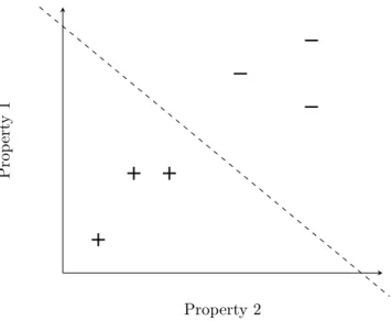
The linear perceptron algorithm was an early model for supervised learning. It was first described by Rosenblatt (1957) and was developed in hardware. The linear perceptron aims to learn a linear function for separating binary class data. This is data for whichy falls into one of two classes. The linear perceptron achieves classification by learning a hyperplane. Intuitively, this is a linear function which aims to divide the training dataset into homogeneous sets, where a set is defined as homogeneous when each of the instances within it have the same target class. This is not possible in all cases.

Figure 2.1 shows an example training set which contains six feature vectors split into two classes, positive and negative. Each instance in the set contains two properties, and the set has been plotted as a scatter with each axis representing a property. The dashed line shows a hyperplane which has succeeded in splitting the dataset. A hyperplane always has one dimension fewer than the number of dimensions of the feature space. As the feature space in figure 2.1 is two-dimensional, the hyperplane can be plotted as a one-dimensional line.

The hyperplane in a perceptron is determined by a vector of weights, w, and a bias b. The weight vector controls the plane’s slope and the bias controls its distance from the origin. Together, w and b form θ for the linear perceptron. Many implementations combine w and b

into a single vector by placing the bias in index 0 of the weight vector and assuming that the value ofx0 is 1 for each instance. Thus,w∈RM+1. This scheme will be assumed for the rest of this section. Note that in this case,θ andw have the same meaning; however,θ is intended as

(10)

Property 2

Prop

ert

y

1

Figure 2.1: An example dataset containing instances split into two target classes. Each axis represents a feature. The dataset is homogeneously split by a linear hyperplane.

σ(P₎ b x1 xi xM w1 wi wM ˆ y

Figure 2.2: A visual depiction of a linear perceptron.

an abstract notion whereasw is concrete. Depicted visually in figure 2.2, the decision function of a linear perceptron can be defined as:

ˆ

y=f(x,θ) =σ(w|x). (2.7)

Henceσis a function used to convert the output ofw|xinto a prediction. The linear perceptron exists in numerous forms, many of which use a differentσ. This thesis will look at the choice of

σfor perceptrons trained for logistic regression and for large margin perceptrons. Each of these will become relevant further into this chapter.

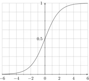
Logistic regression is a form of linear perceptron which aims to learn a function which not only classifies instances but can also estimate the probability that an instance falls within a class. Logistic regression is a misleading name for the model as it is typically used for classification. Assuming that the two possible classes have been labelled as +1 and −1, the output of the perceptron is an estimate of the probability that an instance falls into the class defined as +1. Thus yˆ= P(y = 1|x). If there is a high probability then yˆwill be close to 1, if it is unlikely

(11)

−6 −4 −2 0 2 4 6 0.5

1

Figure 2.3: The logistic function.

then it will be close to 0. To achieve this, a perceptron can use the logistic function for the link functionσ:

σ(a) = 1

1 +e−a (2.8)

Figure 2.3 provides a visual depiction of the logistic function. To convert between this probability and a target class, post-processing ofyˆis required. Ifyˆpasses a threshold, then it may be classified as+1, else it is classified as−1. This threshold is often set at 0.5, though it does not have to be. As explained in section 2.1, a supervised learner must undergo training before it can be used for prediction. This involves optimising θ against the error function E, which in turn means minimising a loss function for each of the instances in the training dataset. The loss function used in logistic regression is log loss, also known as cross-entropy. It follows the form

`(ˆy, y) =−[ylog ˆy+ (1−y) log(1−yˆ)]. (2.9) The log loss function is largest when the perceptron is confident in a prediction which is incorrect. Even correct classifications incur some loss if they are not confident. If the correct class is predicted with a probability of one then`(ˆy, y) = 0.

The full error function for the training set is the sum of the log loss for each of the instances inD. An interesting property of this error function is that once minimised, the perceptron will be optimised for estimating probabilities rather than for classification. A classifier trained for logistic regression is willing to sacrifice its ability to classify correctly in order to improve its ability to estimate probability. Because of this, the logistic function may be less well suited to tasks which require only classification without needing an estimate of probability. Better suited is a large margin perceptron. Instead of the logistic function, large margin perceptrons use the identity function forσ:

ˆ

y=σ(a) =a. (2.10)

Unlike the logistic function, the identity function does not restrictyˆto a value between 0 and 1. Thus it is not possible to calculate probability using this form of the large margin perceptron. As with the logistic function, post-processing ofyˆis required to obtain a classification. Asyˆis no

(12)

Algorithm 1Gradient Descent 1: Inputs:D, η

2: Initialise:w

3: while not convergeddo 4: w:=w−η_∂∂_wE(w,D)

5: end while

longer restricted, it is common practice to classify instances with positiveyˆas+1and instances with negativeyˆas −1. Because the large margin perceptron does not predict a probability, the log loss function should not be used to measure loss. Instead, the large margin perceptron uses the hinge loss function:

`(ˆy, y) = max(0,−y, yˆ ). (2.11) Using hinge loss, correctly classified instances incur no loss, else loss is linear. An interesting property of hinge loss is that once combined intoE, it creates a convex function with respect to

θ. The significance of this will become apparent shortly.

Until now, little detail has been provided on the algorithm for minimising loss. It has been assumed that this algorithm exists, but no explanation or implementation has been provided. In reality, development of the minimisation algorithm is one of the main challenges faced when developing a model. For the perceptron, a number of learning algorithms exist. Perhaps the most commonly used of these is gradient descent. Gradient descent is an iterative algorithm which aims to minimiseEby taking repeated steps in the direction of the negative gradient with respect toθ:

θ:=θ−η ∂

∂θE(θ,D), (2.12)

where η is a learning rate, used to control how aggressively the perceptron updates θ at each iteration. In effect, gradient descent ‘walks’ down the slope of the error function until a stopping criterion is met. At this point, it is said that the perceptron has converged. A common choice of stopping criterion is to halt training when the gradient becomes close to zero. The full gradient descent algorithm may be seen in algorithm 1.

Choosingη is an important step in the implementation of a perceptron. If the selected value is too large then the perceptron may not converge and if it is too small then convergence will take considerably longer than necessary. In general, it is better to pickηcautiously as, given enough time, a classifier which has been trained with an excessively low η will converge to a solution close to the solution obtained by a classifier trained with an optimumη. The same cannot be said for a classifier which has been trained with anη which is too large.

Gradient descent is only guaranteed to find the optimumθfor convex functions. Non-convex functions prove difficult due to the fact that there may be local minima. These are points of the function which are the minimum of a local region of parameter space but are not necessarily the minimum globally. Gradient descent will continue descending a local minimum until it converges, though the solution will likely be non-optimal. As the hinge loss function is a convex, large margin perceptrons are unaffected by local minima.

The version of gradient descent described above is named batch gradient descent because the training dataset may be considered a batch of data. Alternatives to batch gradient descent are stochastic and mini-batch gradient descent. In stochastic gradient descent, only a single

(13)

instance is presented at a time, and the gradient calculated with respect to this instance only. The instances are presented in a random order. Stochastic gradient descent makes many small steps towards the minimum, rather than fewer large steps. It is more resistant to local minima than batch gradient descent since the direction of the gradient is more variable. However, the variability makes it more difficult to reach a gradient of zero in stochastic gradient descent. Mini-batch gradient descent is a compromise in which a configured number of instances are used to calculate the gradient per iteration. The configured number is named the batch size. The aim is to select a batch size which allows the algorithm to escape shallow local minima, while also being able to reach a gradient of near zero when a deeper local minimum is found. With a batch size ofN, mini-batch gradient descent is equivalent to batch gradient descent, and with a batch size of one, it is equivalent to stochastic gradient descent. In practice, correctly tuned mini-batch gradient descent will often outperform batch or stochastic gradient descent in training time and accuracy. The batch size may be selected through cross-validation.

Gradient descent is not the only possible method of training a perceptron. Quasi-Newton methods are a class of optimisation methods which pursue the stationary point where gradient equals zero. They assume that the current gradient is the side of a quadratic bowl and use second order information to jump straight to the point which achieves the minimum of the bowl. This is usually an incorrect assumption, but in practice, the method often allows a classifier to take larger steps towards the minimum than in gradient descent. Quasi-Newton methods are particularly advantageous for optimising error landscapes with long valleys in which gradient descent performs poorly. BFGS (Fletcher, 1987) is one such implementation of a Quasi-Newton method. It is iterative by nature and uses an approximation of the inverse Hessian to reduce training time. Like gradient descent, Quasi-Newton methods are susceptible to traversing local minima.

2.3 Multi-layer Perceptrons

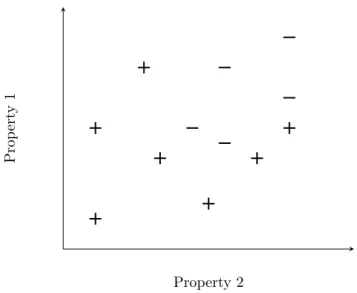
Figure 2.1 in the previous section introduces an example dataset, and shows how a hyperplane can be used to homogeneously separate the instance space. However, this example is simplistic and does not reflect real-life datasets. For most real datasets, it is impossible to separate all of the datapoints into homogeneous sections using a linear hyperplane. For example, consider the dataset in figure 2.4. There is no way that the points can be separated using a one-dimensional line. The dataset is not linearly-separable.

Due to its simplistic design, the linear perceptron may only ever model a linear decision boundary. While this is acceptable for some datasets, many require a more complex function. Resultantly, the perceptron often performs poorly compared to more flexible learners. Fortu-nately, an adjustment may be made to the linear perceptron which allows it to model non-linear data. This requires additional terminology. Figure 2.2 in the previous section depicts a linear perceptron visually and within this depiction is a processing unit which calculates the output of

σ. This processing unit may be called a node.

To model a non-linear decision boundary, the perceptron may introduce additional nodes. These nodes must be stacked so that the output of at least two nodes are used as the input of another node. Moreover, the function used asσfor the additional nodes cannot be linear. The multilayer perceptron (MLP) (Werbos, 1982) is a model which requires that these additional

(14)

Property 2

Prop

ert

y

1

Figure 2.4: An example training dataset containing two classes which cannot be split homoge-neously using a linear hyperplane.

σ σ σ σ x1 xi xM ˆ y

Figure 2.5: A multilayer perceptron with a single output node.

nodes are arranged into layers such that at least one layer of nodes exists between the input feature vector, and an output node used to calculate a finalyˆ. This additional layer is named the hidden layer and the feature vector is named the input layer. Figure 2.5 shows a MLP with a single hidden layer. A MLP may have any number of hidden layers, however, for reasons which will be explained as the section progresses, there is rarely a benefit to having more than two. There is no restriction on the number of output nodes in a MLP, for example, a common scheme used for classification in multiclass problems is one-hot encoding. In one-hot encoding, an output node is added for each of the target classes in T. Each node represents a class, and after running the decision function, the output node with the highest score is the class which is chosen as the classification. A common implementation of MLP is the fully-connected MLP. This is an implementation which requires that each of the nodes within each layer, including the input layer, are connected to each of the nodes in the subsequent layer. This is depicted in figure 2.6. From this point forward, discussions will assume that a MLP is fully connected unless stated otherwise.

(15)

wij

Layer(n−1)

Layer (n)

ai

aj

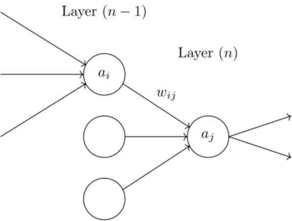
Figure 2.6: A visualisation of a MLP to display notation.

following layer by a set of weights, however, the number of connections is substantially greater. Describing the decision function of a MLP requires further notation. First, a label(n)is required to describe which layer of the network is in discussion. The input layer is described as layer(0)

and the total number of layers will be notated as L. The number of nodes within layer (n)

will be notated N(n)_{. Also required is a notation for describing the output of} _σ_{, known as the}

activation, for a node. For this,awill be used. The MLP requiresL −1weight arrays such that

w(n)_{contains the weights between each of the nodes in layer}₍_n₎_{and layer} ₍_n_{+ 1)}_{. Each array}

must now be a two-dimensional matrix rather than a vector and the weight between two nodes,

i andj, will be given by w_ij(n). Putting this together, the activation of a nodej in layer (n)is given by: a(_jn)=σ   N(n−1) X i=0 w(_ijn−1)a(_in−1)  . (2.13)

It is assumed that the bias is stored in connectionw0jand that and that the activationa

(n−1)

0 =

1. The score yˆis found by recursively calculating activations, starting from nodes in the input layer and finishing at the output layer. Since the output layer may contain multiple nodes, y

and yˆ may be vectors. The function σ may be any differentiable function, with an additional restriction for nodes in the hidden layer, that the function must be non-linear. Therefore the logistic function is an acceptable choice for hidden nodes, however, the identity function does not meet the criteria for hidden layers. A commonσused by MLPs is the hyperbolic tangent:

σ(a) = tanh(a). (2.14)

When plotted, the hyperbolic tangent has a similar shape to the logistic function, however the function ranges between values of 1 and -1 rather than 0 and 1. In many cases, the symmetry around the origin helps with the speed of convergence, as explained in (LeCun et al., 1998b). The derivative of the hyperbolic tangent may be calculated as _{∂ a}∂ tanh(a) = 1−tanh(a)2. The hyperbolic tangent cannot be used in the output layer if a probability estimation is required, however, there is no restriction forσto be the same function in each layer. It is common to see the hyperbolic tangent used in the hidden layers, and the logistic function used in the output layer in order to estimate probabilities.

The loss function in a MLP depends directly on the output of nodes in the final layer, although this will depend on nodes in the hidden layers. As previously stated, the output layer may contain

(16)

multiple nodes, and soy andyˆare vectors rather than single values. The loss function must be updated accordingly. Although more complex schemes exist, a simple yet effective technique is to sum the loss of each of the nodes in the output layer. For example, the MLP variant of log loss for classification may be defined:

`(ˆy, y) =

N(L)

X

j

(yjlog ˆyj+ (1−yj) log(1−yˆj)). (2.15)

A MLP may be trained using a form of gradient descent named backpropagation. As with the decision algorithm, this is a recursive algorithm which updates layers one at a time. It requires that the gradient ofEis calculated with respect to each of the layers in the MLP using the chain rule. Details of how this is achieved may be found in (Werbos, 1974). Once the gradient has been calculated with respect to each of the layers, the standard gradient descent algorithm defined in 2.12 may be used to update the weight vector within each layer. As with gradient descent, backpropagation may take many iterations before convergence. Methods like momentum (Polyak, 1964) and adaptive learning rates (Schaul et al., 2013) aim to reduce the required number of iterations.

As previously described, adding a hidden layer of nodes allows a MLP to model non-linear decision functions. In fact, it was proved in (Cybenko, 1989) that it is possible to approximate any decision region to arbitrary accuracy using a single hidden layer and any continuous sigmoidalσ. This makes the MLP a flexible model for learning complex functions. However, as a result of this, the MLP is susceptible to overfitting. Section 2.1 described two methods to avoid overfitting. The first of these was to reduce the number of tunable parameters inθand the second was to add regularisation to the model. Both of these techniques are applicable to the MLP. In the context of a MLP,θ can be thought of as the combination of each of the weight vectors. The number of required weights depends on the number of connections between nodes. The more connections, the more flexible a MLP is, and the more likely it is to overfit. The number of connections is controlled by the number of nodes, and by the complexity of the arrangement of these nodes. In particular, the number of hidden layers has a profound effect on the complexity. Adding an extra layer of nodes will usually increase the number of connections by an amount greater than would occur if the same number of nodes were added to an existing layer. Choosing the layout of a MLP, also called the topology, is arguably the main challenge in successful implementation. The optimum layout is different between problems and depends on the intrinsic complexity of the dataset. Cross-validation can be used to select the number of nodes and layers.

The second technique to avoid overfitting is to add a regularisation term. This is an artificial adjustment to the error function which aims to reduce the size of items withinθ. For MLPs, this is often achieved by using weight decay regularisation. As touched upon in section 2.1, weight decay regularisation follows the form:

Ereg(θ) =

X

i=1

θ_i2. (2.16)

The value of this term, multiplied by a weighting, is added to the total of the error function so that learning will tend towards weight vectors with low values. This helps to guard a MLP from overfitting because the non-linearities which cause overfitting are more significant when features are large.

(17)

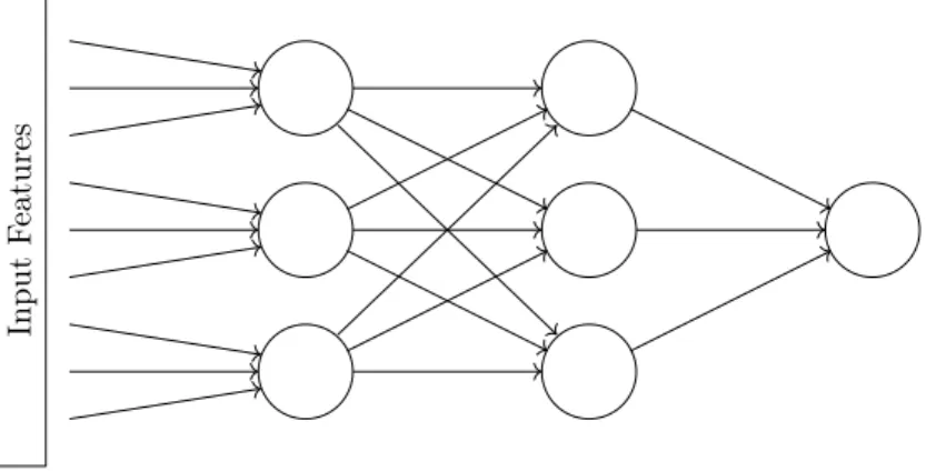
Input

F

eatures

Figure 2.7: A neural network for which the first layer is sparsely connected. The hidden layers remain fully connected.

2.4 Convolutional Neural Networks

The MLP is part of a wider class of model named the Neural Network. Like the MLP, all Neural Networks consists of nodes which are connected by weights, however, there is no restriction for layers to be fully connected. The Convolutional Neural Network (CNN) (LeCun et al., 1989) (LeCun et al., 2015) is a type of Neural Network which specialises in tasks that exhibit local correlation of features, for example, image recognition.

These are tasks for which features within close spatial proximity to one another can form recognisable value patterns. In such tasks, more information may be gained by using the value of a feature relative to its neighbours than can be gained from its value alone. The CNN utilises this additional information with the addition of sparsely connected layers, named convolutional layers, where a layer is considered sparse if it has nodes which are only connected to a local subset of nodes in the following layer. In addition, connections within a convolutional layer are reused at multiple points along the input. To achieve this, the convolutional weights, known collectively as the filter and denoted byf, ‘slide’ along the input, considering only a subset of features at any one time. The number of features which the filter slides over is known as the stride. CNNs still make use of a fully connected network for classification, however, the convolutional layers stand between the input and the fully connected network, as shown in figure 2.7. For a CNN with a single convolutional layer that is the first layer in the network, and for which the stride is one, the number of nodes in the first fully connected layer must equal |x| − |f|+ 1. For this network, the input,u, to a particular node,i, in the first fully connected layer is given by:

u(1)_i = |f|

X

j=0

xi+jfj. (2.17)

When performed at each possible index, this operation is named convolution and is denoted by the∗operator. The output of convolution is called the feature map and is symbolised asu:

(18)

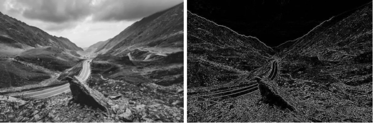
Figure 2.8: An example convolution of an image with an edge detecting kernel. Left shows the original image and right shows the feature map after convolution with a filter containing the values: h−1−1 8−1−1−1

−1−1−1

i

.

CNNs have been shown to be especially effective at image classification tasks, with state-of-the-art results in many benchmark datasets, for example, MNIST (LeCun et al., 1998a), ImageNet Large Scale Visual Recognition Challenge (Russakovsky et al., 2015) and Caltech 256 (Griffin et al., 2007). In these datasets, the input features are the pixel values of each image. Instead of storing features in a vector, they are stored in a tensor which has a rank of two or three, with the third dimension containing colour values if they exist. The filter is usually two-dimensional and during convolution it advances horizontally and vertically. Typically, a different filter is trained for each of the colour channels. The aim of convolution is to extract the defining features of an image, for example, a particular texture or the edges of an object. The movement of the filter allows a CNN to find such features anywhere within an image. It improves the shift invariance of the model which allows it to generalise more effectively to unseen data. As a positive byproduct of sharing filter coefficients, the number of connections in a CNN is low when compared to fully connected networks of an equivalent size. Figure 2.8 shows an example of convolution on a real image.

The description given so far has used a single filter in the convolutional layer, however, many real-world implementations, including the three given above, use multiple stacked filters per layer. Each filter can be trained to highlight a different defining feature. When an input is passed to the convolutional layer, each of the filters is convolved with the input. If the layer contains k

filters, then the output will containkfeature maps. As well as having multiple filters per layer, a network may have multiple convolutional layers. In this case, each of the filters in convolutional layer l(n) _{are applied to each of the feature maps which were created by layer} _l(n−1)_{. Given a}

network with two convolutional layers which are the first two layers of the network, the total number of feature maps after the second layer of convolution is given byk(0)_×_k(1)_{. Assuming}

that each of the filters within l(n) _{is of equal cardinality and that this cardinality is denoted}

|f(n)|, the total number of tunable filter weights is given byk(0)× |f(0)|+k(0)×k(1)× |f(1)|. As the number of filters per layer increases, the total size of a network can quickly become unmanageable. For this reason, many networks include subsampling layers. These are layers which forcibly reduce the size of feature maps by tactically removing non-essential information.

(19)

A common method to achieve this is max-pooling. Max-pooling divides a feature map into partitions and then carries forward only the greatest value from each partition into the proceeding layer. The partitions are named pooling windows and for image recognition tasks, each pooling window has a width and a height. Ordinarily, the widths and heights are uniform throughout the image and are referred to as the pooling width, pw, and pooling height, ph. Max-pooling

reduces the size of feature maps by a factor ofpw×phassuming that the width and height of a

feature map are divisible bypw andphrespectively. Although the same number of feature maps

are passed to the fully connected network, the reduction in the size of feature maps substantially decreases the number of nodes required in the fully connected network. As well as decreasing the number of tunable parameters, max-pooling provides a degree of shift invariance as the output of a pooling window will be consistent regardless of where a feature lies within the pooling window. During backpropagation, the gradient only propagates back through the maximum feature within each pooling window. An alternative to max-pooling is average-pooling, whereby the output is the average over all of the nodes in the pooling window.

The idea of using sliding filters in a neural network is first described in (LeCun et al., 1989), although the networks are described as constrained rather than convolutional, and no subsam-pling method is employed. It was nine years later in (LeCun et al., 1998a) that CNNs close to their current form are described. The network in (LeCun et al., 1998a) combines the ideas of local receptive fields, shared filter weights and subsampling. It applies the network to an image classification problem, named MNIST, which contains 70,000 images of handwritten numeric characters split into ten target classes. The data is split into a training set, containing 60,000 images, and a test set which contains the remaining 10,000. Each image is of size 28x28, and the contents are centred by mass. The CNN developed in (LeCun et al., 1998a), dubbed LeNet-5, contains seven layers excluding the input layer. Of these, two are convolutional layers, two are subsampling layers and the remaining three form a fully connected network. The convolutional and subsampling layers alternate before feeding into the fully connected network. Using this topology, LeNet-5 is able to achieve a generalisation error of 0.95%, compared to 2.95% obtained by the highest performing fully-connected network described in the paper. In the time since its publication in 1998, MNIST has become a popular dataset for benchmarking models. At this time of writing, a variant of the CNN still yields the greatest accuracy on the dataset, achieving 0.21% generalisation error (Wan et al., 2013a).

2.5 Support Vector Machines

The Support Vector Machine (SVM) (Boser et al., 1992) (Cristianini and Shawe-Taylor, 2000) is a supervised model for separating binary data-sets wherey∈ {−1,1}. It is an influential and prevalent model with many parallels to the linear perceptron. Like the perceptron, a SVM aims to find a linear hyperplane for classification. It shares the same decision function:

ˆ

y=w|x+b, (2.19)

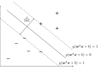
however, the method used for training differs. During training, SVMs focus on separating the data points which are nearest to the decision boundary. These are named the support vectors. The rationale for this is that optimal separation of the most difficult datapoints is equivalent to the optimal separation of the entire dataset. Figure 2.9 shows an example of a hyperplane which achieves maximum separation of the support vectors. Above and below are the planes at which

(20)

2 kwk

y(w|_x₊_b_{) = 1}

y(w|x+b) = 0

y(w|_x₊_b_{) = 1}

Figure 2.9: A dataset which has been split homogeneously by a SVM hyperplane. The hyperplane achieves maximum separation of most difficult instances within the two target classes. Above and below are the planes, named the boundaries, at whichy(w|_x₊_b_{) = 1}_.

fall. This is not by chance, it is a requirement of w. The distance between the boundaries is known as the margin and is given by _k_w2_k. Maximising the margin will maximise the distance between support vectors. Therefore, the optimum w is the smallest w which can satisfy the requirements. On linearly separable data, this can be achieved by minimising the hard-margin error function:

E=kwk2 subject to yi(w|xi+b)≥1 ∀i, (2.20)

where{xi, yi} are the training data.

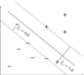
When the data is not linearly separable, the hard-margin SVM error function will fail to converge as there is no way to satisfy all of the constraints. Instead, the soft-margin error function may be used. The soft-margin function introduces a leniency to the constraints with the addition of slack variablesξ. The slack variables alter the constraints such thaty(w|xi+b)

may equal 1−ξi, rather than 1. If 0 < ξi <1, then xi must fall within the margin but still

falls on the correct side of the decision boundary. Ifξi>1then thexi falls on the incorrect side

of the decision boundary. The introduction ofξ prevents outliers from controlling the decision boundary, as illustrated in figure 2.10. The soft-margin error function can be defined:

E=kwk2+C

N

X

j

ξj subject to yi(w|xi+b)≥1−ξi ∀i, (2.21)

where C is a regularisation parameter to control the extent to which the decision boundary is constrained. A small C will allow the SVM to easily ignore constraints, resulting in a wide margin, but with many support vectors violating the boundaries. A largeC heavily penalises the cost of support vectors within the boundaries, resulting in a narrow margin. With very large C, the soft-margin error function is equivalent to the hard-margin function. Both the hard and soft margin error functions are convex and a number of methods exist to optimise these. Perhaps the simplest of these conceptually is to treat the error function as a constrained quadratic programming problem and to solve this directly using Lagrange multipliers, or using an algorithm such as Sequential Minimal Optimisation (SMO) (Platt, 1998). Alternatively, the

(21)

ξ_i = 0_.₆ ξ_j = 1_. 6

Figure 2.10: An example hyperplane which has been learned by optimising the soft margin error function. Two of the instances fall within the margin because the slack variables relax the SVM constraints.

optimisation problem may be reformulated into an unconstrained version:

E=kwk2+C

N

X

i

max(0,1−yi(w|xi+b)). (2.22)

The unconstrained optimisation is equivalent to the large-margin perceptron optimisation prob-lem, but with the addition of L22 regularisation on w. Therefore, learning may be achieved

by using gradient based optimisation approaches, for example, the Pegasos algorithm (Shalev-Shwartz et al., 2011).

The soft-margin error function allows a SVM to converge on data which is not linearly sep-arable but it does not increase the expressive power of the classifier. The formulation described is only flexible enough to describe a linear decision boundary. However, with adjustments, it is possible for the SVM to describe arbitrarily complex boundaries. Moreover, it is possible to do this while retaining the aim of learning a linear hyperplane. Instead of learning a more complex shape than a plane, the SVM opts to alter the input features so that a plane is adequate for classification. It does this by using a function named a feature mapping, denoted byφ. The aim of aφis to map a feature vector into a new vector with a greater number of dimensions:

φ(x) =φ       x1 .. . xM      =    x1 .. . xM0   , (2.23)

whereM0≥M. M0 may even be infinite. The hope is that in the higher dimensional space, the data can be more easily separated. The feature mapping may be considered a preprocessing step before classification by a linear hyperplane. Thus, the decision function is linear with respect to

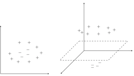
φ(x) but non-linear with respect to x. Figure 2.11 shows an example feature mapping which maps between_R2_and

R3. InR2the datapoints are inseparable, however, by mapping the inputs into _R3_{, it is possible to separate the dataset using a linear hyperplane. When using a feature}

(22)

+ + + + + + + + + − − − − + + + +₊ + + + + − −₋−

Figure 2.11: Applying an example feature mapping to a dataset containing two-dimensional instances. In two dimensions the dataset is not linearly separable but in three dimensions it is.

mapping, the decision function becomes:

ˆ

y=w|φ(x) +b. (2.24)

Likewise, the error functions seen in equations (2.20), (2.21) and (2.22) remain the same, but with all occurrences ofxreplaced byφ(x).

While feature mappings provide the means to classify non-linear data using a SVM, in prac-tice, they can prove too computationally expensive for realistic use. For some datasets, the number of output dimensions required by the mapping function may be infinite. So, instead of explicitly working out the high-dimensional space, many SVM formulations choose to take a shortcut. The SVM formulation which is described above is called the primal form. An alter-native is the dual form. In the dual form, w does not exist as a concrete variable. Instead, it is calculated as a combination of the data such that w = PN

i αiyiφ(xi), where αi is a scalar

which is learned during training. For training instances which are not considered to be support vectors,αi will be close to zero. The dual formulation of the decision function may initially be

defined as: ˆ y= n X i=1 αiyiφ(xi)|φ(x) +b, (2.25)

At this point the dual and primal forms are equivalent, and the issues around computational complexity are still present. The power of the dual form becomes apparent with the addition of a kernel function. Proposed in (Boser et al., 1992), a kernel function,K(xi,xj), can be used

to calculate the output of φ(xi)|φ(xj), while avoiding the need to calculate φ(xi) or φ(xj)

directly. Computationally, this is considerably cheaper in most cases. Using Mercer’s theorem (Mer, 1909), it can be shown that all positive semi-definite kernels are equivalent to an inner product after mapping with someφ. With the addition of a kernel function, the decision function becomes: ˆ y= n X i=1 αiyiK(xi,x) +b, (2.26)

(23)

The simplest kernel function is the linear kernel: K(xi,xj) =x|ixj. In this case, no feature

mapping is performed andφ(x) =x. More common choices are the polynomial kernel:

K(xi,xj) = (x|ixj+ 1)d (2.27)

and the RBF kernel:

K(xi,xj) = exp(−γkxi−xjk2) (2.28)

wheredandγ are parameters which control the complexity of the feature mapping. Even with the addition of a kernel function, the SVM learning algorithm remains convex. Updating the error function for the dual may be achieved by following a similar process to that used to obtain (2.26). For the regularisation term:

kwk2₌ N X i αiyiφ(xi) !|  N X j αjyjφ(xj)   = N X i N X j αiαjyiyjK(xi,xj). (2.29)

Inserting this and the representation of the decision function into the primal error function seen in (2.22) gives: E= N X i N X j αiαjyiyjK(xi,xj) +C N X i max(0,1−yi( N X j αjyjK(xi,xj) +b). (2.30)

However, this is rarely used as the optimisation problem. Instead, it is reframed into an equivalent maximisation problem overαwhich is easier to solve:

N X k αk− 1 2 N X i N X j αiαjyiyjK(xi,xj) subject to 0≤αi ≤C ∀i and N X i αiyi= 0. (2.31)

This is possible due to the representation theorem (Schölkopf et al., 2001) and the fact that the minimisation problem is strongly convex. The solution which solves the dual optimisation problem will also solve the primal problem as long as the Karush-Kuhn-Tucker (KKT) conditions are satisfied (Kuhn and Tucker, 1951).

The SVM implementations discussed so far have been exclusively for binary classification. Although SVM formulations exist which natively support multi-class classification, a more com-mon method for approaching multiclass problems is to use a scheme such as one-versus-one or one-versus-all. In such schemes, no adaption is required to the SVM formulation discussed above. Instead, multiclass is achieved by training multiple classifiers, each designed to classify a partic-ular target or a pair of targets. In a one-versus-all scheme,|T|classifiers are learned, whereT is the set of target values. Each classifier is trained with data which has been relabelled so that all instances of one class havey = +1and any instance which is not of this class has y =−1. To decide the final classification of an instance,yˆis calculated for each of the classifiers, and the class represented by the classifier with the greatestyˆis selected as the output. An alternative scheme is one-versus-one. In this scheme, a classifier is trained for each pair of target classes, resulting in

|T|(|T|−1)

2 classifiers in total. The final classification of an instance is obtained by making a class

prediction using each of the classifiers and then selecting the class with the greatest number of votes. Although one-versus-one requires the creation and training of many more classifiers than one-versus-all, the overall training time is often lower as fewer instances are used to train each classifier.

(24)

2.6 Multiple Kernel Learning

Multiple Kernel Learning (MKL) is an extension to the SVM in which multiple kernel functions are combined into a hybrid. A number of MKL formulations exist, however, all share the rationale that the most effective kernel is unknown and should therefore be learned as part of training. A common form of MKL is where the kernels and their parameters have been predefined and the aim of learning is to decide how they should be combined. The combination function is denoted byC, and it requires a set of weights g:

K(xi,xj,g) =C(g,{km(xi,xj)}Pm=1), (2.32)

where P represents the number of predefined kernels. An example of this formulation is the weighted sum: K(xi,xj,g) = P X m=1 gmkm(xi,xj) (2.33)

This is valid since the sum of Mercer kernels is itself a Mercer kernel. Another category of MKL is where the combination function is already known, and instead, the aim is to optimise the parameters which are integrated into the kernels. For example, learning the optimumγ in the RBF kernel or the degree of a polynomial kernel. Here, the kernel functions themselves require the weights stored ing. Assuming that each kernel function requires a single weight:

K(xi,xj,g) =C({km(xi,xj, gm)}Pm=1). (2.34)

This formulation is integral to the classifier developed later in this work. The error function of an MKL problem may be structured in many ways, for example the formulation of (Rakotomamonjy et al., 2008) may be used for learning the weighted sum, whereas (Chapelle et al., 2002) may be used for learning the internal kernel parameters. A general formulation which flexibly describes a range of MKL problems, including the two mentioned above, is Generalised MKL (GMKL). Described in (Varma and Babu, 2009), GMKL aims to optimise the following function:

min w,b,g 1 2w |_w₊X i l(yi,C(xi)) +r(g) subject to g≥0 (2.35)

wherel is a loss function, for example, hinge loss, andr is a regularisation function which may be any function which is differentiable with respect tog. This error function is equivalent to the SVM primal error function but with additional regularisation of the kernel parameters.

GMKL minimises this function by using an iterative two-step optimisation. First g is fixed while an arbitrary SVM optimisation algorithm is used to learn w, then g is learned using gradient descent whilew is fixed. GMKL aims to minimise the primal function overall but the internal SVM optimiser maximises the dual function with the intention of finding the optimum

α, denoted α∗. After training of the internal SVM is complete,g is optimised by holding α∗

constant and using gradient descent. These two steps repeat until convergence. To optimiseg

using gradient descent, the derivative of the error functionE(w, b,g), defined in equation (2.35), is required. Varma and Babu (2009) show that this gradient may be calculated using:

∂ E ∂ gk = ∂r ∂gk −1 2α ∗|∂H ∂gk α∗, (2.36)

(25)

Algorithm 2Generalised MKL (Varma and Babu, 2009) 1: n←0 2: Initializeg0 _randomly 3: repeat 4: K←k(gn₎ 5: α∗←solve SVM using K. 6: gn_k+1←gn k −s n₍∂r ∂gk− 1 2α ∗|∂H ∂gkα ∗₎

7: Projectgn+1 _{onto the feasible set if any constraints are violated.}

8: n←n+ 1

9: untilConverged

where H is the matrix generated by calculating yiyjK(xi,xj,g)for all combinations ofi and

j. The requirement of a two-step optimisation stems from the fact that this derivate requires values forα∗. After the update ofg, the values found forα∗are no longer optimum and need to be recalculated. In turn, this causesg to become outdated. Therefore GMKL requires a number of iterations before convergence. As the iteration number increases, the size of the updates to

α andg diminish. A step size,s, adds further control to the size of the update ofg. The full GMKL algorithm is presented in Algorithm 2. Unfortunately, optimisation ofg is not generally a convex problem, however, the learning ofw remains convex.

2.7 Conclusion

This chapter has provided the prerequisite information which will be required in chapters 3 and 4. It began with a model agnostic description of machine learning and then provided information on Linear Perceptrons, Multilayer-Perceptrons, Convolutional Neural Networks, Suppor Vector Machines and Multiple Kernel Learning.

To summarise, the linear perceptron is an early model for supervised learning. It is arguably the quintessential model for achieving binary classification. Despite this, the linear perceptron performs poorly on many many real datasets due to the lack of flexibility caused by its inherent linearity. However, it is possible to achieve non-linearity by combining a number of perceptrons into a multi-layer perceptron. The convolutional neural network (CNN) is a further development to the multi-layer perceptron which uses sparse layers to utilise spatial information from its inputs and weight sharing to provide leniency regarding the location of this spatial information. This is useful on many tasks for which the location of features is important, for example, image classification. Resultantly, the CNN has achieved state-of-the-art results on many benchmark datasets.

An alternative model for classification is the support vector machine (SVM). The linear SVM is similar to the linear perceptron, even sharing the same decision function. However, the regularisation which is used during the training of a SVM is designed so that the hyperplane achieves optimum separation of the most difficult datapoints, named the support vectors. It is possible for a SVM to achieve non-linearity by using a kernel function to calculate the inner products of its inputs in a higher dimensional space. Optimisation remains a convex problem by using this method. Multiple kernel learning builds on this by providing an approach which may be used to combine kernel functions into a hybrid. Alternatively, it can be used to optimise

(26)

internal kernel parameters, for example the degree of a polynomial kernel.

The CNN and SVM are essential for understanding the models which are proposed in chapters 3 and 4. In addition, chapter 4 requires knowledge of multiple kernel learning.

(27)

Chapter 3

Linear Convolutional SVMs

Among others, chapter 2 describes two models: the convolutional neural network and the support vector machine. The CNN excels in tasks which exhibit spatially local correlation of features, for example, image classification, however, it suffers from multiple local minima due to the MLP which it uses in the final layers. This thesis presents a method for replacing the MLP in the final layer with a SVM. The convolutional layers may be considered feature extractors before classification with the SVM. The resulting model will be named the Convolutional Support Vector Machine (CSVM). This chapter will describe an approach which may be used in the primal to augment a linear SVM with convolutional layers. The following chapter will describe an alternative approach which may be used in the dual with a kernelised SVM.

The idea of combining support vector machines and convolutional neural networks into a hybrid classifier has been investigated in previous work. In (Huang and LeCun, 2006) a CNN was trained was on the NORB dataset (LeCun et al., 2004) and once training was complete, the final layers were replaced with a SVM. The NORB dataset is an image recognition benchmark dataset containing pictures of children’s toys from many angles. It can be further broken down into two datasets, the uniform set and the jittered-cluttered set. The normalised-uniform set contains centred images of similar size and on a normalised-uniform background, whereas the jittered-cluttered set contains the same images but each has been deliberately perturbed and has been placed on a cluttered background. The hybrid classifier performs well on both datasets: On the jittered-cluttered dataset the hybrid classifier achieves 5.9% error rate, compared to 7.2% for a CNN and 43.3% for a regular SVM. It also achieves 5.9% error rate on the normalised-uniform set, compared to 6.2% for a CNN and 11.6% for a SVM. However, the fact that the fully-connected network is swapped out for a SVM after training, means that the convolutional filter weights are optimised for use with a classifier which is not used at classification time.

Tang (2013) builds upon this approach by proposing a method for training a deep convolu-tional network in conjunction with SVM parameters. This is achieved by replacing the output layer with a set of SVMs, one per target output. Thus, as in (Huang and LeCun, 2006), the inputs to the SVM are the penultimate activations of the neural network. At prediction time, an instance is classified as the target represented by the SVM which gives the greatest output. Each of the SVM weight vectors is learned using gradient descent of the primal loss function, and connection weights in the deep network are learned by using backpropagation from this

(28)

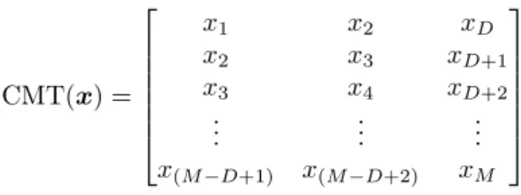
CMT(x) =        x1 x2 xD x2 x3 xD+1 x3 x4 xD+2 .. . ... ... x(M−D+1) x(M−D+2) xM       

Figure 3.1: An example of a convolutional matrix to achieve one-dimensional convolution. M =

|x|andD=|f|. In this exampleD= 3.

initial gradient. The initial gradient is calculated with respect to the penultimate activations of the neural network. As the primal loss is used to calculate gradient, the model is restricted to learning linear SVMs. It is up to the deep neural network to induce non-linearity into the prediction. The model, dubbed DLSVM, achieves a greater generalisation accuracy than a CNN using a softmax output layer on the popular MNIST and CIFAR-10 datasets, and on the ICML 2013 Representation Learning Workshop’s face expression recognition challenge.

This chapter proposes an alternative approach for learning convolutional filter weights in conjunction with a linear SVM weight vector. Instead of using backpropagation, it proposes an iterative, two-step optimisation. Each of the steps executes a convex optimisation. The chapter will begin by looking at the simplest case: a linear CSVM (L-CSVM) with a single convolutional filter, a stride of one and with no subsampling. In this case, the decision function may be defined in the primal as:

ˆ

y=w|(x∗f) +b, (3.1)

where yˆis the predicted target of an instance x, f denotes a convolutional filter, b symbolises the bias andx∗f expresses the convolution operation betweenxandf. The dimension of the weight vector is therefore|w| − |f|+ 1. The convolution operation aims to increase the distance between positive and negative support vectors so that a greater margin is possible.

Training of the L-CSVM may be achieved by making minor alterations to the SVM error function. First, the SVM constraints are altered to take into account the convolution operation, so thatyi(w|(xi∗f) +b)≥1−ξi ∀i. Next, regularisation must be added to the filter weights.

Without regularisation, the filter may grow or shrink without bound. To regularise, the squared

L2-norm is used, as forw. With these changes, the full L-CSVM error function may be defined:

E= λw 2 kwk 2₊λf 2 kfk 2₋ 1 N N X i=1 max{0,(yi(w|(x∗f) +b)}, (3.2)

where λw and λf take the place of C in equation (2.21) in deciding how much the constraints control the decision boundary.

To simplify the task of optimising this error function, this thesis introduces a function which it calls the Convolution Matrix Transformation (CMT). The CMT function takes a feature vector,

x, and transforms it into a new vector whose inner product withf produces the same output as convolvingxwithf directly. The output of CMT(x,f) will be called the convolutional matrix and will be notated byX. Thus X =CMT(x,f). The feature vector may have any number of dimensions, for example, it may be a two-dimensional greyscale image or a three-dimensional colour image. TheXcreated by CMT will be set up to perform convolution over each dimension

(29)

Algorithm 3Two-dimensional CMT Algorithm 1: Inputs: x∈Rm×n,f ∈Rp×q 2: Initialise: X∈R((m−p+1)(n−q+1))×(pq) 3: fori= 0tom-p+ 1do 4: forj= 0ton-q+ 1do 5: fork= 0 topdo 6: forl= 0 toqdo 7: a:=i(n−q+ 1) +j 8: b:=kq+l 9: Xa,b :=x(i+k),(j+l) 10: end for 11: end for 12: end for 13: end for 14: Output: X

in the original image, such that:

CMT(x,f)|f =X|f =x∗f. (3.3) Figure 3.1 shows an example of a convolutional matrix which may achieve one-dimensional con-volution. IfM =|x|andD=|f|then the shape of X is(M−D+ 1)byD. The convolutional matrix to achieve one-dimensional convolution is created by stacking subsets of the original in-stance vector such that the start index of the subset increments by one at each row. ThusXis a staggered matrix containing the elements ofx. To achieve two-dimensional convolution, whereby a two-dimensional filter is convolved with a two-dimensional input vector, a more complex opera-tion is required than staggering to create the convoluopera-tional matrix. In this case, Algorithm 3 may be used. To calculate the output ofx∗f,f must be vectorised. Thus vec(x∗f) =X|vec(f). UsingX instead ofx, the decision function and error function my be written as:

ˆ y=w|X|f+b (3.4) and: E= λw 2 kwk 2₊λf 2 kfk 2₋ 1 N N X i=1 max{0,(yi(w|X|f+b))} (3.5) respectively.

An interesting property of this error function is that if the filter is held fixed, and the convolu-tion logic is extracted into the setup of the dataset, such thatD0={X|_f_}N

i=1, then optimisation

of the weight vector looks like the usual SVM problem. Likewise, if the weight vector is held fixed, and the weight vector arithmetic is encoded into the training data such thatD00={w|X}N

i=1,

then optimisation of the filter again looks like the usual SVM optimisation problem. Therefore learning may be performed as an iterative two-step optimisation; first by trainingwwithf held fixed, and then by training f with w fixed. Both optimisation steps are convex and may be performed with an arbitrary linear SVM training algorithm, for example, SMO (Platt, 1998) or Pegasos (Shalev-Shwartz et al., 2011). Pseudocode for this is presented in Algorithm 4. The algorithm uses a command named SVM. This command calculates and returns the optimum weight vector for a set of inputs using an arbitrary linear SVM algorithm. It is used in step 6 to calculate the SVM weight vector. However, in step 8 it is used to learn the filter coefficients rather than the weight vector. This works as the cardinality of each instance inD00is|f|.

(30)

Algorithm 4L-CSVM Learning Algorithm 1: Inputs:D, λw, λf

2: Initialise:w,f

3: Xi :=CMT(Di,f) ∀i

4: while not convergeddo 5: D0:={Xi|f}Ni=1 6: w, b:=SVM(D0, λw) 7: D00:={w|_X_i_}N i=1 8: f :=SVM(D00, λf) 9: end while

3.1 Experimental Results: MNIST

Section 2.4 describes the MNIST image classification dataset (LeCun et al., 1998a). MNIST is widely used as a benchmark dataset and is freely available to researchers. Therefore, it is a natural dataset on which to test the L-CSVM. The results of the L-CSVM are compared against results of a linear SVM, and an equivalent CNN with a single convolutional filter.

3.1.1 Results

In order to implement Algorithm 4, a SVM implementation needed to be chosen. The classifier developed in this research used a custom implementation of the Pegasos algorithm written in Java. Pegasos was chosen due to its ability to converge rapidly in the linear case. The implementation included the optional projection step, although this was found to have little impact on the properties of the trained classifier, nor on the training time. Multiclass classification was achieved using a one-versus-one scheme, and, for simplicity, λw and λf were shared between all of the classifiers rather than selected per classifier. The MNIST target classes are the numerical digits from 0 to 9, and a different filter was learned for each pair of targets, resulting in 45 distinct filters. Each filter was of size5×5. Cross-validation was used to tune λw andλf. The 60,000 training instances were split into 50,000 for training and 10,000 for validation. With so many instances available per target class, k-fold validation was deemed unnecessary. A heatmap of cross-validation results can be seen in figure 3.2. The highest performing classifier hadλw= 0.1 and λf = 0.1, and so these are the parameters which are used to determine generalisation accuracy.

As a comparison, a linear SVM without convolutional filters and a linear implementation of a CNN were also implemented. The SVM used the same custom implementation of Pegasos. In this implementation, the only parameter which required tuning wasλw, for which the optimum value was found to be0.1. The CNN was also implemented in Java and used the open source Deeplearning4j library (Skymind, 2014). The architecture of the CNN was designed to be as equivalent as possible to the L-CSVM. It had a single convolutional filter, also of size5×5, did not perform subsampling, and did not contain any hidden layers. Thus, the convolutional feature maps fed directly into a linear classifier, as was the case in the L-CSVM. It used the sigmoid function in the output layer and used log loss to calculate error gradient. For training, stochastic gradient descent was used with Nesterov’s Accelerated Gradient (NAG) (Nesterov, 1983) momen-tum. NAG momentum achieved superior classification results and resulted in a lower training

(31)

Figure 3.2: A heatmap of cross-validation results on the training and validation sets. Cross-validation aimed to learn effective values ofλf andλw.

MNIST Results

Model Training accuracy % Testing accuracy % Linear SVM 93.57±0.053 93.68±0.15 Linear CNN 91.92±0.089 91.60±0.15

L-CSVM 94.06±0.072 94.09±0.14

Table 3.1: Accuracy averaged over ten runs on the MNIST testing set using a variety of classifiers. The error is estimated using the standard deviation.

time than equivalent networks using conventional momentum, and without momentum. The two variables which required tuning were the learning and regularisation rates. Cross-validation on the validation set found the optimum values to be10−3and 10−5 respectively.

Table 3.1 shows the results of each of the classifiers. Accuracies are averaged over ten runs of the model and the error estimate shows the standard deviation. Accuracy was chosen as the performance metric over precision, recall or F1-score as a correct classification of all target classes is of equal importance. As can be seen from the results, the L-CSVM achieves an accu-racy of 94.09% on the testing set which is the highest accuaccu-racy of each of the tested classifiers. Interestingly, the linear SVM outperforms the linear CNN. This suggests that a linear classifier generalises sufficiently well on MNIST that it does not fully benefit from the additional general-isability provided by the convolutional filter. This is further evidenced by the fact that the SVM achieves a similar accuracy on the testing set as it does on the training set. The conclusion may be drawn that in the linear case, the convex properties of the SVM learning algorithm are more important than the shift invariance provided by a single convolutional filter. Chapter 4 explores whether this is the case for more flexible classifiers.