Distributed Machine Learning Framework: New
Algorithms and Theoretical Foundation
by
Zhouyuan Huo
BS, Zhejiang University, 2014
Submitted to the Graduate Faculty of
the Swanson School of Engineering in partial fulfillment
of the requirements for the degree of
Doctor of Philosophy
University of Pittsburgh
2020
UNIVERSITY OF PITTSBURGH SWANSON SCHOOL OF ENGINEERING
This dissertation was presented by
Zhouyuan Huo
It was defended on April 1, 2020 and approved by
Heng Huang, PhD, John A. Jurenko Endowed Professor, Department of Electrical and Computer Engineering
Liang Zhan, PhD, Assistant Professor, Department of Electrical and Computer Engineering Zhi-Hong Mao, PhD, Professor, Department of Electrical and Computer Engineering Wei Gao, PhD, Associate Professor, Department of Electrical and Computer Engineering
Wei Chen, PhD, Associate Professor, The School of Medicine, Department of Pediatrics Dissertation Director: Heng Huang, PhD, John A. Jurenko Endowed Professor,
Copyright c by Zhouyuan Huo 2020
Distributed Machine Learning Framework: New Algorithms and Theoretical Foundation
Zhouyuan Huo, PhD University of Pittsburgh, 2020
Machine learning is gaining fresh momentum, and has helped us to enhance not only many industrial and professional processes but also our everyday living. The recent success of machine learning relies heavily on the surge of big data, big models, and big computing. However, inefficient algorithms restrict the applications of machine learning to big data min-ing tasks. In terms of big data, serious concerns, such as communication overhead and data privacy, should be rigorously addressed when we train models using large amounts of data located on multiple devices. In terms of the big model, it is still an underexplored research area if a model is too big to train on a single device. To address these challenging problems, this thesis is focusing on designing new large-scale machine learning models, efficiently op-timizing and training methods for big data mining, and studying new discoveries in both theory and applications.
For the challenges raised by big data, we proposed several new asynchronous distributed stochastic gradient descent or coordinate descent methods for efficiently solving convex and non-convex problems. We also designed new large-batch training methods for deep learning models to reduce the computation time significantly with better generalization performance. For the challenges raised by the big model, We scaled up the deep learning models by parallelizing the layer-wise computations with a theoretical guarantee, which is the first algorithm breaking the lock of backpropagation such that the large model can be dramatically accelerated.
Table of Contents Preface . . . xi 1.0 Introduction . . . 1 1.1 Background . . . 1 1.2 Contribution . . . 2 1.3 Notation . . . 3 1.4 Thesis Organization . . . 3
2.0 Asynchronous Mini-batch Gradient Descent with Variance Reduction for Non-Convex Optimization . . . 5
2.1 Motivation . . . 5 2.2 Preliminaries . . . 7 2.3 Shared-Memory Architecture . . . 8 2.3.1 Algorithm Description . . . 8 2.3.2 Convergence Analysis . . . 9 2.4 Distributed-Memory Architecture . . . 16 2.4.1 Algorithm Description . . . 16 2.4.2 Convergence Analysis . . . 16 2.5 Experimental Results . . . 22 2.5.1 Shared-Memory Architecture . . . 23 2.5.2 Distributed-Memory Architecture . . . 27
3.0 Asynchronous Dual Free Stochastic Dual Coordinate Ascent for Dis-tributed Data Mining . . . 29
3.1 Motivation . . . 29
3.2 Preliminaries . . . 31
3.2.1 Stochastic Dual Coordinate Ascent . . . 32
3.2.2 Dual Free Stochastic Dual Coordinate Ascent . . . 32
3.3.1 Update Global Variable on Server . . . 34
3.3.2 Update Local Variable on Worker . . . 35
3.4 Convergence Analysis . . . 37
3.4.1 Convex Case . . . 38
3.4.2 Non-convex Case . . . 41
3.5 Experimental Results . . . 43
3.5.1 Convex Case . . . 43
3.5.1.1 Convergence of Duality Gap . . . 44
3.5.1.2 Speedup . . . 44
3.5.2 Non-convex Case . . . 46
4.0 Large Batch Training Does Not Need Warmup . . . 48
4.1 Motivation . . . 48
4.2 Preliminaries . . . 49
4.3 Complete Layer-Wise Adaptive Rate Scaling . . . 51
4.3.1 Complete Layer-Wise Adaptive Rate Scaling . . . 51
4.3.2 Fine-Grained Micro-Steps and Assumptions . . . 52
4.3.3 Convergence Guarantees of Two Gradient-Based Methods . . . 54
4.3.4 Discussions About the Convergence of mNAG . . . 69
4.4 Experimental Results . . . 70
4.4.1 Why LARS? . . . 71
4.4.2 Linear Learning Rate Scaling . . . 72
4.4.3 One Hypothesis About Warmup . . . 73
4.4.4 Warmup is Not Necessary . . . 75
5.0 Decoupled Parallel Backpropagation with Convergence Guarantee. . . 78
5.1 Motivation . . . 78
5.4 Convergence Analysis . . . 85
5.4.1 Fixed Learning Rate . . . 90
5.4.2 Diminishing Learning Rate . . . 91
5.5 Experimental Results . . . 92
5.5.1 Comparison of BP, DNI and DDG . . . 94
5.5.2 Optimizing Deeper Neural Networks . . . 97
5.5.3 Scaling the Number of GPUs . . . 99
6.0 Training Neural Networks Using Features Replay . . . 101
6.1 Motivation . . . 101
6.2 Preliminaries . . . 102
6.3 Features Replay . . . 104
6.3.1 Problem Reformulation . . . 105
6.3.2 Breaking Dependencies by Replaying Features . . . 105
6.4 Convergence Analysis . . . 107 6.5 Experimental Results . . . 111 6.5.1 Experimental Setting . . . 111 6.5.2 Sufficient Direction . . . 112 6.5.3 Performance Comparisons . . . 114 7.0 Conclusion . . . 117 Bibliography . . . 119
List of Tables
1 Notations used in thesis. . . 4 2 Experimental datasets from LIBSVM. . . 44 3 Comparisons of computation time when the network is sequentially distributed
across K GPUs. . . 83 4 Neural networks architectural details in the experiments. . . 92 5 The best Top 1 classification accuracy for ResNet-56 and ResNet-110 on the
test data of CIFAR-10 and CIFAR-100. . . 100 6 Comparisons of memory consumption of the neural network with L layers,
which is divided into K modules. . . 114 7 Best testing error rates of the compared methods on CIFAR-10 and CIFAR-100
List of Figures
1 Comparison of three methods: SGD, SVRG, SGDSVRG on MNIST dataset. 23 2 Speedup of Shared-AsySVRG on a machine with different number of threads
from 1 to 32. . . 24 3 Comparison of three methods: SGD, SVRG, SGDSVRG on CIFAR-10. . . . 25 4 Speedup of Distributed-AsySVRG on multiple machines from 1 to 10. . . 26 5 Distributed asynchronous dual free stochastic dual coordinate ascent for
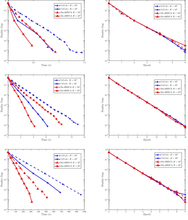
pa-rameter server framework. . . 31 6 Convergence of duality gap of compared methods in terms of time and epoch
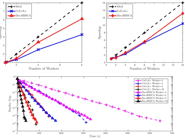
for IJCNN1, COVTYPE, RCV1 respectively. . . 45 7 Time speedup in terms of the number of workers. Row 1 left: IJCNN1; Row 1
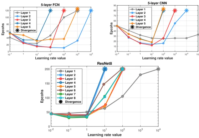
right: COVTYPE; Row 2: RCV1. . . 46 8 Suboptimum convergence of compared methods in terms of time. . . 47 9 Learning rate upper bound for 5-layer FCN, 5-layer CNN, and 8-layer ResNet. 70 10 Training loss and Top-1 testing accuracy of training ResNet56 and VGG11
(with batch normalization layer) on CIFAR-10. . . 71 11 Learning rate schedule. . . 72 12 Variation of variance for 10 epochs. We train 5-layer FCN and 5-layer CNN
with sigmoid activation on MNIST. . . 74 13 Comparison between LARS (with gradual warmup) and CLARS algorithm. . 75 14 Comparison between LARS and CLARS training ResNet50, DenseNet121, and
MobileNetv2 on ImageNet. . . 77 15 Procedure of the backpropagation algorithm. . . 79 16 Procedure of the decoupled parallel backpropagation algorithm. . . 80 17 Training and testing curves of loss function regarding epochs for ResNet-8 on
18 Training and testing curves of Top 1 classification accuracies regarding epochs for ResNet-8 on CIFAR-10. . . 94 19 Training and testing curves regarding epochs for ResNet-8 on CIFAR-10. . . 95 20 Training and testing loss curves for ResNet-110 on CIFAR-10 using multiple
GPUs. . . 96 21 Computation time and the best Top 1 accuracy for ResNet-110 on the test
data of CIFAR-10. . . 97 22 Training and testing curves for ResNet-56 and ResNet-110 on CIFAR-10. . . 98 23 Training and testing curves for ResNet-56 and ResNet-110 on CIFAR-100. . 99 24 Illustrations of the backward pass of the backpropagation algorithm (BP)
de-coupled neural interface (DNI) and dede-coupled parallel backpropagation (DDG). 103 25 Backward pass of Features Replay Algorithm. . . 104 26 Sufficient direction constant for ResNet164 and ResNet101 on CIFAR-10. . . 111 27 Memory consumption for ResNet164, ResNet101 and ResNet152. . . 112 28 Training and testing curves for ResNet-164, ResNet101 and ResNet152 on
Preface
First and foremost, I would like to thank my Ph.D. advisor, Professor Heng Huang. Heng has been an exceptional advisor and I have been very fortunate to do research under his supervision for the six years of Ph.D. journey. Heng is highly self-motivated and I am deeply impressed by his tremendous passion for research. In the past six years, Heng has been always ready to offer me extremely visionary advice and the most generous support. I learned from Heng how to discover a problem, how to define this problem, and how to solve this problem. I feel very lucky that I can start and pursue my research career under the supervision of Professor Heng Huang.
I would also like to thank Professor Zhi-Hong Mao, Professor Wei Gao, Professor Liang Zhan, and Professor Wei Chen for being on my Ph.D. committee. I really appreciate their great advice and guidance for my research direction. I feel honored to get the inspiring instructions from them and am grateful to the committee members for their valuable time and help.
I want to thank every member in the Pitt Data Science Lab. Thanks Dr. Feiping Nie, Dr. Bin Gu and Dr. Feihu Huang for their guidance, insightful discussions and collaboration during my Ph.D. study. I would thank my friends and lab mates: An, De, Xin, Guodong, Xiaoqian, Hongchang, Kamran, Yanfu, Runxue, Wenhan, Shangqian. I feel very lucky to be a member of such a wonderful research group and it was my pleasure working together with you all.
It has been an honor for me to work with many great collaborators in the academia or when I was a summer intern in the industry lab. I would like to thank Zachary Garrett, Jakub Koneˇcn´y, Brendan McMahan, Peter Kairouz from Google Research and Hao Jiang, Lin Liang, Quanzeng You from Microsoft Research for advising and helping me in the internship projects. I also enjoyed hanging out and collaborations with other interns, Liang Yang and Ziteng Sun.
Finally, I give special thanks to my families, especially parents, grandparents and Qian. Thank you for raising me up and I can’t accomplish what I did without your love and
support. Thanks for your understanding and love in the past years. Because of you, I can get over obstacles in my way. Because of you, I never stray too far from the sidewalk.
1.0 Introduction
1.1 Background
The phenomenal progress of machine learning and the explosive growth of big data have been accelerating the trend of world development. While this vision is expected to generate many disruptive business and social benefits, it presents many unprecedented challenges. In terms of model, current deep learning models are not well designed or too small to learn human knowledge. In terms of data, serious concerns such as data privacy should be rigorously addressed when we train models using amounts of data generated on personal devices. In terms of optimization, training giant neural networks or training models on the device cause new difficulties for current optimization algorithms.
The scalability and efficiency have been the notorious bottlenecks of some machine learn-ing models, constrainlearn-ing them from belearn-ing applied to big data. Large amounts of data can boost machine learning models to obtain remarkable predictive capabilities. When data are distributed across devices, however, training models suffer from heavy computation, slow communication, or lacking convergence guarantee. An efficient distributed optimiza-tion method should make sure that models will converge to soluoptimiza-tions in the end with fewer computations and faster communication.
To reduce the communication overhead, asynchronous parallel algorithms for stochastic optimization have received huge successes in theory and practice recently. Because there is no need of synchronization between workers, asynchronous methods often have better perfor-mance than synchronous methods. [80] proposed the first asynchronous parallel stochastic gradient descent (SGD) algorithm known as Hogwild!. [39] proposed an asynchronous par-allel SGD algorithm with the SVRG variance reduction technique.
The growth of neural network depth is one of the most critical factors contributing to the success of deep learning. It has been verified both in practice and in theory that the more significant number of parameters of a neural network can facilitate its learning abil-ity. For example, the current state-of-the-art models in various applications are giant neural
networks: convolutional neural networks with over 1000 layers for image classification, or Transformer networks with 1.6B parameters for natural language understanding. However, such giant neural networks cannot fit in a single training device. Besides, current optimiza-tion algorithms cannot make full use of computing resources, wasting much energy, and affecting the environment. It remains a key problem in deep learning that the deep neural networks with millions of or even billions of parameters cannot fit in a single training device, e.g., GPU or TPU. In many applications such as image classification, object detection and language models, If we allocate and train the parameters of a neural network on multiple GPUs, backward locking in backpropagation algorithm becomes the bottleneck of making full use of computing resources, leading to serious loss of money and energy. The backward locking constrains us from updating models in parallel and fully leveraging the computing resources.
The goal of this thesis is to propose new distributed optimization algorithms and provide theoretical foundation to address the challenges in training distributed machine learning problems using model parallelism and data parallelism.
1.2 Contribution
We summarize our contribution as follows:
• We provide the first theoretical analysis on the convergence rate of asynchronous mini-batch gradient descent with variance reduction (AsySVRG) for non-convex optimization. We prove that both methods can converge with a rate of O(1/T) for non-convex optimization, and linear speedup is accessible when we increase the number of workers.
• We address two challenging issues in previous primal-dual distributed optimization meth-ods: firstly, Dis-dfSDCA does not rely on the dual formulation, and can be used to solve
• We propose a novel Complete Layer-wise Adaptive Rate Scaling (CLARS) algorithm for large-batch training. We also analyze the convergence rate of the proposed method by introducing a new fine-grained analysis of gradient-based methods. Based on our analysis, we bridge the gap and illustrate the theoretical insights for three popular large-batch training techniques, including linear learning rate scaling, gradual warmup, and layer-wise adaptive rate scaling.
• We decouple the backpropagation algorithm using delayed gradients, and show that the backward locking is removed when we split the networks into multiple modules. Then, we utilize decoupled parallel backpropagation in two stochastic methods and prove that our method guarantees convergence to critical points for the non-convex problem.
• We propose a novel parallel-objective formulation for the objective function of the neural network. After that, we introduce features replay algorithm and prove that it is guaranteed to converge to critical points for the non-convex problem under certain conditions. Finally, we apply our method to training deep convolutional neural networks, and the experimental results show that the proposed method achieves faster convergence, lower memory consump-tion, and better generalization error than compared methods.
1.3 Notation
Unless specified otherwise, the notations used in this thesis are listed in Table 1.
1.4 Thesis Organization
The rest of the thesis is organized as follows. In Chapter 2, we introduce a new asyn-chronous mini-batch gradient descent with variance reduction for non-convex optimization. In Chapter 3, we design a new distributed dual-free SDCA algorithm to address two chal-lenging issues in previous primal-dual distributed optimization methods. In Chapter 4, we propose a novel Complete Layer-wise Adaptive Rate Scaling (CLARS) algorithm for
large-Table 1: Notations used in thesis. f objective function w model parameter ∇f gradient n number of examples d number of parameters T number of iterations
batch training. In Chapter 5, we decouple the backpropagation algorithm using delayed gradients and parallelize the neural network training if the model is too big. Next in Chap-ter 6 we propose a features replay algorithm and show that it outperforms compared model parallelism algorithms. Finally, we conclude the thesis in Chapter 7.
2.0 Asynchronous Mini-batch Gradient Descent with Variance Reduction for Non-Convex Optimization
2.1 Motivation
With the boom of data, training machine learning model with large-scale datasets be-comes a challenging problem. Basing on batch gradient descent (GD) method, researchers propose stochastic gradient descent (SGD) method or mini-batch gradient descent method to relieve the complexity of computation in each iteration and reduce the total time com-plexity for optimization [73, 55, 24, 26, 9]. Due to efficiency, SGD method has been widely used to solve different kinds of large-scale machine learning problems, including both convex and non-convex. However, because we use stochastic gradient to approximate full gradient in the process, a decreasing learning rate has to be applied to guarantee convergence, or it is very easy to diverge from the optimal solution. Thus, it leads to a sub-linear convergence rate of O(1/T) on strongly convex problem. Recently, stochastic variance reduced gradient (SVRG) [46] and its variants, such as SAGA[17], m2SGD[51], have gained much attention in stochastic optimization. Through reusing the previously computed first order gradient information, these methods are able to reduce the variance of gradient approximation in the optimization and are proved to have linear convergence rate on strongly convex problem. After that, SVRG is then applied to solve non-convex problem [4, 81], and it is proved to have a faster sub-linear convergence rate of O(1/T). Experiments are conducted on neural networks and their results also validate that it outperforms SGD method for non-convex optimization.
Serial algorithm is not able to make good use of computation resource. Therefore, parallel algorithms are introduced to further speedup the computation task, including synchronous optimization and asynchronous optimization. Because there is no need of synchronization between workers, asynchronous methods often have better performance. Asynchronous par-allelism has been successfully applied to speedup many state-of-the-art optimization algo-rithms, such as SGD [80, 59], stochastic coordinate descent (SCD) [64], SVRG [109] and
Du-alFreeSDCA [40]. There are mainly two kinds of distributed architectures, one is distributed-memory architecture on multiple machines [2, 59, 108, 16, 109] and the other one is shared-memory architecture on a multi-core machine [80, 111, 112]. Deep learning is a typical situation where asynchronous SGD and its variants have gained great success[56, 16, 59, 75]. It is known that deep neural network always has large set of parameters and trains with large-scale datasets.
Recently, asynchronous SVRG method has been implemented and studied on distributed-memory architecture [109] and shared-distributed-memory architecture [111]. It is proved that asyn-chronous SVRG method has linear convergence rate on strongly convex problem. Mini-batch gradient is implemented in the experiments, while it is missing in their proof. Further, there is no theoretical analysis of convergence rate for asynchronous SVRG on non-convex problem yet.
In this chapter, we provide the convergence analysis of asynchronous mini-batch gradi-ent descgradi-ent with variance reduction method (asySVRG) for non-convex optimization. Two different algorithms and analysis are proposed on two different distributed architectures, one is shared-memory architecture and the other is distributed-memory architecture. The key difference between these two categories lies on that distributed-memory architecture can ensure the atomicity of reading and writing the whole vector of x, while the shared-memory architecture can usually just ensure atomic reading and writing on a single coordinate of x
[59]. We implement asySVRG on two different architectures and analyze their convergence rate based on the mini-batch setting. We prove that asySVRG can get convergence rate of
O(1/T) on both architectures. Besides, we also prove that linear speedup is accessible when we increase the number of workers until reaching an upper bound.
We list our main contributions as follows:
• We extend asynchronous shared-memory SVRG method to solve non-convex problem. Our Shared-AsySVRG on shared-memory architecture has faster convergence rate than
gence rate than AsySGD. We prove that Distributed-AsySVRG has a convergence rate of O(1/T) for non-convex optimization.
• Both of Shared-AsySVRG and Distributed-AsySVRG have linear speedup when we in-crease the number of threads in a shared-memory architecture or workers in a distributed-memory architecture until reaching an upper bound.
2.2 Preliminaries
We consider the following empirical loss minimization problem: min x∈Rd f(w) = 1 n n X i=1 fi(w), (2.1)
wheref(w) andfi(w) are Lipschitz smooth, they are not necessarily convex. In this chapter, we assume both of them are non-convex.
Following the proof in [59, 81, 4] for non-convex optimization, we use the weighted average of the `2 norm of full gradient||∇f(w)||2 as metric to analyze its convergence property. For further analysis, throughout this chapter, we make the following assumptions for problem (2.1). All of them are very common assumptions in the theoretical analysis for asynchronous stochastic gradient descent method.
Assumption 2.2.1. Independence: All random samples i are selected randomly and in-dependently to each other.
Assumption 2.2.2. Unbiased Gradient: The stochastic gradient ∇fi(w) is unbiased: E[∇fi(w)] =∇f(w). (2.2) Assumption 2.2.3. Lipschitz Gradient: We say∇f(w) is Lipschitz continuous, and it holds:
||∇f(w)− ∇f(v)||2 ≤L||w−v||2. (2.3)
Throughout, we also assume that the function ∇fi(w) is also Lipschitz continuous, so that
Assumption 2.2.4. Maximum Time Delay: Time delay variable τ of parameters in each worker is upper bounded, namely maxτ ≤∆. In practice, ∆is related with the number of workers.
2.3 Shared-Memory Architecture
In this section, we propose AsySVRG method for shared-memory architecture, and prove that it converges with rateO(1/T). It is proved that SVRG has a convergence rate ofO(1/T) on non-convex problem [81, 4]. In this section, we follow the convergence analysis in [81], and extends it to asynchronous optimization on shared-memory architecture.
2.3.1 Algorithm Description
Following the setting in [59], we define one iteration as a modification on any single component of x in the shared memory. We use xs+1t to denote the value of parameter x in the shared memory after (ms+t) iterations, and Equation (2.4) represents the update rule of parameter x in iterationt: (wt+1s+1)kt = (w s+1 t )kt −η(v s+1 t )kt, (2.4)
where kt ∈ {1, ..., d} is a random index of component in w ∈ Rd, and learning rate η is constant. Descent direction vts+1 is defined as follows:
vs+1t = 1 |It| X it∈It ∇fit( ˆw s+1 t )− ∇fit( ˜w s) +∇f( ˜ws) , (2.5)
where ˜ws denotes a snapshot ofw after everym iterations. itdenotes the index of a sample, and It is index set of mini-batch samples, and mini-batch size is |It|. The definition of ˆws+1t
Algorithm 1 Shared-AsySVRG Initializew0 ∈Rd.
for s= 0,1,2, , .., S−1 do ˜
ws←ws;
Compute full gradient∇f( ˜ws)← 1 n
n
P
i=1
∇fi( ˜ws); Parallel Computation on Multiple Threads for t= 0,1,2, ..., m−1do
Randomly select mini-batch It from {1, ....n}; Compute vts+1: vs+1t ← 1 |It| P it∈It ∇fit( ˆw s+1 t )− ∇fit( ˜w s) +∇f( ˜ws) ; Randomly select kt from {1, ..., d};
Update (wt+1s+1)kt: (w s+1 t+1)kt ←(w s+1 t )kt −η(v s+1 t )kt; end for ws+1 ←ws+1 m ; end for
whereJ(t)∈ {t−1, ...., t−∆}is a subset of previous iterations, ∆ is the upper bound of time delay. In Algorithm 1, we summarize the Shared-AsySVRG on shared-memory architecture.
2.3.2 Convergence Analysis
In this section, we prove that our proposed Shared-AsySVRG method has a sub-linear convergence rate of O(1/T) on non-convex problem. Different from AsySGD method, we are able to bound the variance of gradient update vs+1t because of the variance reduction technique. And it is crucial for our convergence analysis.
Lemma 2.3.1. As per the definition of the variance reduced gradientvts+1 in Equation (2.5), we define, us+1t = 1 |It| X it∈It ∇fit(w s+1 t )− ∇fit( ˜w s) +∇f( ˜ws) . (2.7)
We have the following inequality: m−1 X t=0 E||vts+1|| 2 ≤ 2d d−2L2∆2η2 m−1 X t=0 E||us+1t || 2 . (2.8) where E||us+1 t ||2
is upper bounded following [82]:
E||us+1t || 2 ≤2E||∇f(ws+1t )||2 +2L 2 b E ||ws+1t −w˜s||2 . (2.9)
Proof of Corollary 2.3.1: As per the definitions of vts+1 (2.5) and us+1t (2.7): E||vs+1t || 2 = E||vs+1 t −u s+1 t +u s+1 t || 2 ≤ 2E||vs+1 t −u s+1 t || 2 + 2E||us+1 t || 2 = 2E " ||1 b X it∈It ∇fit( ˆw s+1 t,it )− ∇fit(w s+1 t )|| 2 # + 2E||us+1t ||2 ≤ 2L 2 b X it∈It E||wˆt,is+1t −w s+1 t || 2 + 2E||us+1 t || 2 ≤ 2L 2 b X it∈It E || X j∈J(t,it) (wjs+1−ws+1j+1)kj|| 2 + 2E ||us+1 t || 2 ≤ 2L 2∆η2 bd X it∈It X j∈J(t,it) E||vs+1j || 2 + 2E ||us+1 t || 2 , (2.10)
where the first, third and last inequality follows from ||a1 +...+an||2 ≤n n
P
i=1
||ai||2. Second inequality follows from Lipschitz smoothness of f(w). Then sum over E||vts+1||2
in one epoch, we get the following inequality,
m−1 X t=0 E||vs+1t || 2 ≤ m−1 X t=0 2L2∆η2 bd X it∈It X j∈J(t,it) E||vjs+1|| 2 + 2E||us+1t ||2 ≤ 2L 2∆2η2 d m−1 X t=0 E||vs+1t || 2 + 2 m−1 X t=0 E||us+1t || 2 . (2.11)
From Lemma 2.3.1, we know that the variance of vts+1 goes to zero when we reach the optimal solution if it exists. Thus, we can maintain learning rate as a constant in the optimization. Therefore, our Shared-AsySVRG has a faster convergence rate as follows: Theorem 2.3.1. Suppose all assumptions of f(w) satisfy. Let cm = 0, learning rate η > 0
is constant, βt = β > 0, b = |It| denotes the size of mini-batch samples in each iteration.
We define: ct =ct+1(1 + ηβt d + 4L2η2 (d−2L2∆2η2)b) + 4L2 (d−2L2∆2η2)b( L2∆2η3 2d + η2L 2 ), (2.13) Γt = η 2d − 4 d−2L2∆2η2( L2∆2η3 2d + η2L 2 +ct+1η 2), (2.14)
such that Γt >0 for 0≤ t≤ m−1. Define γ = mintΓt, and w∗ is the optimal solution for non-convex problem. Then, Shared-AsySVRG algorithm has the following convergence rate in iteration T: 1 T S−1 X s=0 m−1 X t=0 E||∇f(ws+1t )||2 ≤ E[f(w 0)−f(w∗)] T γ . (2.15)
Proof of Theorem 2.3.1: At first, we derive the upper bound ofE||wt+1s+1−w˜s||2
: E||wt+1s+1−w˜s||2 =E||ws+1 t+1 −ws+1t +wts+1−w˜s||2 =E||ws+1 t+1 −ws+1t ||2+||wts+1−w˜s||2+ 2 ws+1t+1 −wts+1, wts+1−w˜s =E " η2 d||v s+1 t ||2+||ws+1t −w˜s||2− 2η d * 1 b X it∈It ∇f( ˆwt,is+1t ), ws+1t −w˜s +# ≤ η 2 dE ||vts+1||2 + 2η d E " 1 2βt ||1 b X it∈It ∇f( ˆwt,is+1t )||2+ βt 2||w s+1 t −w˜ s||2 # +E||wts+1−w˜s||2 = η 2 d E ||vs+1 t || 2 + η dβtE " ||1 b X it∈It ∇f( ˆwt,is+1 t )|| 2 # + (1 + ηβt d )E ||ws+1 t −w˜ s||2 , (2.16)
where the inequality follows from ha, bi ≤ 1 2(a
2+b2). Then we know that
Ef(ws+1t+1)
is also upper bounded:
Ef(wt+1s+1) ≤E f(wts+1) + ∇f(wts+1), ws+1t+1 −ws+1t + L 2||w s+1 t+1 −w s+1 t || 2 =Ef(ws+1t )− η dE "* ∇f(ws+1t ),1 b X it∈It ∇f( ˆws+1t,it ) +# +η 2L 2d E ||vs+1 t ||2 =Ef(ws+1t )− η 2dE ||∇f(wts+1)||2+||1 b X it∈It ∇f( ˆws+1t,it )||2 − ||∇f(ws+1t )−1 b X it∈It ∇f( ˆwt,is+1t )||2 +η 2L 2d E ||vs+1 t ||2 , (2.17)
where the first inequality follows from Lipschitz continuity of f(w).
E " ||∇f(ws+1t )−1 b X it∈It ∇f( ˆwt,is+1t )||2 # ≤ L 2 b X it∈It E||ws+1t −wˆt,is+1t || 2 = L 2 b X it∈It E || X j∈J(t,it) (ws+1j −wj+1s+1)||2 ≤ L 2∆ b X it∈It X j∈J(t,it) E||ws+1j −w s+1 j+1|| 2 ≤ L 2∆η2 bd X it∈It X j∈J(t,it) E||vjs+1|| 2 , (2.18)
where the first inequality follows from Lipschitz continuity of f(w). ∆ denotes the upper bound of time delay. From (2.17) and (2.18), it is to derive the following inequality:
Following the proof in [81], we define Lyapunov function (this nice proof approach was first introduced in [81]): Rs+1t =Ef(wts+1) +ct||wts+1−w˜s||2
.From the definition of Lya-punov function, and inequalities in (2.16) and (2.19):
Rs+1t+1 ≤E f(wts+1) − η 2dE ||∇f(ws+1t )||2 − η 2dE " ||1 b X it∈It ∇f( ˆws+1t,i t )|| 2 # + η 2L 2d E ||vs+1 t || 2 +L 2∆η3 2bd2 X it∈It X j∈J(t,it) E||vs+1j || 2 +ct+1 " η2 dE ||vs+1 t || 2 + (1 + ηβt d )E ||ws+1 t −w˜ s||2 + η dβtE " ||1 b X it∈It ∇f( ˆwt,is+1t )||2 ## ≤E f(wts+1)− η 2dE ||∇f(ws+1t )||2 + L 2∆η3 2bd2 X it∈It X j∈J(t,it) E||vs+1j || 2 + (η 2L 2d + ct+1η2 d )E ||vts+1||2 +ct+1(1 + ηβt d )E ||ws+1t −w˜s||2 , (2.20) where we assume 12 ≥ ct+1
βt . As per Corollary 2.3.1, we sum up R
s+1 t+1 fromt= 0 to m−1, m−1 X t=0 Rs+1t+1 ≤ m−1 X t=0 Ef(ws+1t ) − η 2dE ||∇f(wts+1)||2 +L 2∆η3 2bd2 X it∈It X j∈J(t,it) E||vjs+1|| 2 + (η 2L 2d + ct+1η2 d )E ||vs+1 t || 2 +ct+1(1 + ηβt d )E ||ws+1 t −w˜ s||2 ≤ m−1 X t=0 Ef(ws+1t ) − η 2dE ||∇f(wts+1)||2 +ct+1(1 + ηβt d )E ||ws+1 t −w˜ s||2 + (L 2∆2η3 2d2 + η2L 2d + ct+1η2 d )E ||vs+1 t ||2 ≤ m−1 X t=0 Ef(ws+1t ) − η 2dE ||∇f(wts+1)||2 +ct+1(1 + ηβt d )E ||ws+1 t −w˜s||2 + 2d d−2L2∆2η2( L2∆2η3 2d2 + η2L 2d + ct+1η2 d )E ||us+1t ||2 ≤ m−1 X t=0 Rts+1− m−1 X t=0 ΓtE||∇f(ws+1t )|| 2 , (2.21) where ct=ct+1(1 + ηβt d ) + 4L2 (d−2L2∆2η2)b( L2∆2η3 2d + η2L 2 +ct+1η 2 ), (2.22) Γt= η 2d − 4 d−2L2∆2η2( L2∆2η3 2d + η2L 2 +ct+1η 2 ). (2.23)
Setting cm = 0, ˜ws+1 = ws+1m , and γ = min Γt, then Rms+1 = E[f(wms+1)] = E[f( ˜ws+1)] and Rs+10 =Ef(w0s+1)=E[f( ˜ws)]. Thus we can get,
m−1 X t=0 E||∇f(wts+1)|| 2 ≤ E[f( ˜w s)−f( ˜ws+1)] γ . (2.24)
Summing up all epochs, and define w0 as initial point and w∗ as optimal solution, we have the final inequality:
1 T S−1 X s=0 m−1 X t=0 E||∇f(ws+1t )|| 2 ≤ E[f(w 0)−f(w∗)] T γ . (2.25)
Now, we prove that our method has a convergence rate of O(1/T) if problem is non-convex. If we representγ with known parameters, we have the following theorem.
Theorem 2.3.2. Suppose all assumptions of f(w) satisfy. Let η = u0b
Lnα, where 0 < u0 <1
and0< α≤1, β = 2L, m=bdnα
6u0bcand T is the number of total iterations. If the maximum
time delay ∆ satisfies the following condition:
∆2 <min{ d 2u0b ,3d−28u0bd 28u2 0b2 }, (2.26)
there exists universal constant u0 and σ, such that it holds γ ≥ dLnσbα and
1 T S−1 X s=0 m−1 X t=0 E||∇f(ws+1t )|| 2 ≤ dLn α E[f(w0)−f(w∗)] bT σ . (2.27)
Proof of Theorem 2.3.2: Following the proof in [81], we setcm = 0, η= Lnu0bα, βt=β = 2L, 0< u0 <1, and 0 < α <1.
In the final inequality, we constrain that dnα ≤dn2α−2∆2u2
0b2, and it is easy to satisfy when n is large. We set m =bdnα
6u0bc, and from the recurrence formula of ct, we have:
c0 = 2L2 (d−2L2∆2η2)b L2∆2η3 d +η 2L (1 +θ)m−1 θ = 2L u30∆2b3 n3α + u20b2d n2α (d−2L2∆2η2)2u0b2 dnα + 4u2 0b2 dn2α−2∆2u2 0b2 d ((1 +θ)m−1) ≤ L(u0b∆ 2+d) 3d ((1 +θ) m−1) ≤ L(u0b∆ 2+d) 3d (e−1). (2.29)
where the final inequality follows from that (1+1 l)
lis increasing forl > 0, and lim l→∞(1+
1 l)
l=e. From the proof in Theorem 2.3.1, we know that c0 ≤ β2 =L,thus ∆2 ≤ 2ud0b. ctis decreasing with respect to t, and c0 is also upper bounded.
γ = min t Γt ≥ η 2d − 4 d−2L2∆2η2( L2∆2η3 2d + η2L 2 +c0η 2 ) ≥ η 2d − 4nα d ( L2∆2η3 2d + η2L 2 +c0η 2) ≥ 1 2− 14u2 0b2∆2+ 14u0bd 3d η d ≥ σb dLnα. (2.30)
There exists a small value σ, an it is independent of n. The final inequality holds if 1 2 > 14u2 0b2∆2+14u0bd 3d . Above all, if ∆ 2 <min{ d 2u0b, 3d−28u0bd 28u2 0b2
}, we have the conclusion that, 1 T S−1 X s=0 m−1 X t=0 E||∇f(ws+1t )||2 ≤ dLn α E[f( ˜w0)−f( ˜w∗)] T σb . (2.31)
In (2.27), we can find out that the convergence rate has nothing to do with maximum time delay ∆, if it is upper bounded. Thus in a specific domain, the negative effect of using stale information of parameter w for approximating gradient evaluation vanishes, and a linear speedup is accessible when we increase the number of threads.
2.4 Distributed-Memory Architecture
In this section, we propose Distributed-AsySVRG algorithm for distributed-memory ar-chitecture, and prove that it converges with rate O(1/T) on non-convex problem.
2.4.1 Algorithm Description
In each iteration, parameter w is updated through the following update rule,
ws+1t+1 =wts+1−ηvts+1, (2.32)
where learning rateη is constant,vs+1t represents variance reduced gradient, and it is defined as follows: vs+1t = 1 |It| X it∈It ∇fit(w s+1 t−τ)− ∇fit( ˜w s ) +∇f( ˜ws), (2.33)
where ˜ws means a snapshot of w after every m iterations, and ws+1
t−τ denotes the current parameter used to compute gradient in the worker. it denotes the index of a sample, τ denotes time delay of parameter in the worker, and mini-batch size is |It|. Suppose there are K workers in total, and the number of dataset in worker k is nk. We summarize the Distributed-AsySVRG on distributed-memory architecture in the Algorithm 2 and Algorithm 3, Algorithm 2 shows operations in server node, and Algorithm 3 shows operations in worker node.
Algorithm 2 Distributed-AsySVRG Server Node Initializew0 ∈Rd.
for s= 0,1,2, , .., S−1 do ˜
ws←ws;
Broadcast ˜ws to all workers;
Receive and compute: ∇f( ˜ws)← 1 n
K
P
k=1
∇kf( ˜ws); Broadcast∇f( ˜ws) to all workers;
for t= 0,1,2, ..., m−1do
Receive variance reduced gradient vts+1 from worker; Update wt+1s+1 ←wts+1−ηvts+1;
end for
ws+1 ←ws+1m ; end for
Theorem 2.4.1. Suppose all assumptions of f(w) satisfy. Let cm = 0, learning rate η > 0
is constant, βt =β >0, b denotes the size of mini-batch. We define the following equations
regarding ct as follows: ct=ct+1 1 +ηβt+ 4L2η2 (1−2L2∆2η2)b + 4L 2 (1−2L2∆2η2)b L2∆2η3 2 + η2L 2 , (2.34) and Γt as follows: Γt= η 2 − 4 (1−2L2∆2η2)( L2∆2η3 2 + η2L 2 +ct+1η 2), (2.35)
where the requirements are satisfied that Γt >0 for 0≤t ≤m−1. Define γ = mintΓt,
w∗ is the optimal solution for non-convex problem. Then, we have the following convergence rate in iteration T: 1 T S−1 X s=0 m−1 X t=0 E||∇f(ws+1t )|| 2 ≤ E[f(w 0)−f(w∗)] T γ . (2.36)
Algorithm 3 Distributed-AsySVRG Worker Node k
if flag is True then
Receive parameter ˜ws from server;
Compute and send full gradient∇kf( ˜ws):
∇kf( ˜ws) = Pnk
i=1
∇if( ˜ws) ;
Receive full gradient ∇f( ˜ws) from server; else
Receive parameterws+1t−τ from server;
Randomly select mini-batchIt from {1, ..., nk}; Compute vts+1 and send it to server:
vts+1← 1 |It| P it∈It ∇fit(w s+1 t−τ)− ∇fit( ˜w s) +∇f( ˜ws) ; end if Proof of Theorem 2.4.1: E||wt+1s+1−w˜s||2 =E||ws+1 t+1 −ws+1t +wts+1−w˜s||2 =E||ws+1 t+1 −ws+1t ||2+||wts+1−w˜s||2+ 2 wt+1s+1−wts+1, ws+1t −w˜s =E " η2||vs+1 t || 2+||ws+1 t −w˜ s||2−2η * 1 b X it∈It ∇f(ws+1t−τi), ws+1t −w˜s +# ≤η2E||vts+1||2 + 2ηE " 1 2βt ||1 b X it∈It ∇f(ws+1t−τi)||2+ βt 2||w s+1 t −w˜ s||2 # +E||ws+1t −w˜s||2 =η2E||vs+1 t ||2 + (1 +ηβt)E ||ws+1 t −w˜s||2 + η βtE " ||1 b X it∈It ∇f(wt−τs+1i)||2 # , (2.37) where the first inequality follows 2ha, bi ≤ ||a||2+||b||2.
f(ws+1)≤
f(ws+1) +∇f(ws+1), ws+1−ws+1+ L||ws+1−ws+1||2
where the first inequality follows from Lipschitz continuity off(w). Then we know the upper bound of ||∇f(ws+1t )− 1 b P it∈It ∇f(wt−τs+1i)||2 as follows: ||∇f(ws+1t )− 1 b X it∈It ∇f(ws+1t−τi)||2 ≤ 1 b X it∈It ||∇f(wts+1)− ∇f(wt−τs+1i)||2 ≤ L 2 b X it∈It ||ws+1 t −w s+1 t−τi|| 2 ≤ L 2∆ b X it∈It t−1 X j=t−τi ||ws+1 j −w s+1 j+1|| 2 = L 2∆η2 b X it∈It t−1 X j=t−τi ||vs+1 j || 2, (2.39)
where the second inequality follows from Lipschitz continuity off(w). ∆ denotes the upper bound of time delay. τ ≤∆. Above all, we have the following inequality,
Ef(ws+1t+1) ≤E f(ws+1t )− η 2E ||∇f(ws+1t )||2 − η 2E " ||1 b X i∈It ∇f(ws+1t−τ i)|| 2 # +η 2L 2 E ||vs+1 t || 2 +L 2∆η3 2b X i∈It t−1 X j=t−τi E||vs+1j || 2 . (2.40)
Following the definition of Rt+1s+1,
Rs+1t+1 =E f(ws+1t+1) +ct+1||wt+1s+1−w˜ s||2 ≤E f(ws+1t ) − η 2E ||∇f(wts+1)||2 − η 2E " ||1 b X i∈It ∇f(wt−τs+1 i)|| 2 # + η 2L 2 E ||vs+1t ||2 +L 2∆η3 2b X i∈It t−1 X j=t−τi E||vjs+1|| 2 +ct+1 " η2E||vs+1 t ||2 + (1 +ηβt)E ||ws+1 t −w˜s||2 + η βtE " ||1 b X i∈It ∇f(wt−τs+1i)||2 ## ≤E f(ws+1t )− η 2E ||∇f(wts+1)||2 +L 2∆η3 2b X i∈It t−1 X j=t−τi E||vs+1j || 2 + (η 2L 2 +ct+1η 2) E||vts+1|| 2 +ct+1(1 +ηβt)E ||ws+1 t −w˜ s||2 . (2.41)
In the final inequality, we make (η2 − ct+1η
βt ) >0. Then we sum over R
s+1
t+1, the following inequality holds that:
m−1 X t=0 Rs+1t+1 ≤ m−1 X t=0 Ef(wts+1) − η 2E ||∇f(wts+1)||2 +L 2∆η3 2b X i∈It t−1 X j=t−τi E||vjs+1|| 2 + (η 2L 2 +ct+1η 2 )E||vs+1t ||2 +ct+1(1 +ηβt)E||wts+1−w˜s||2 ≤ m−1 X t=0 Ef(ws+1t ) − η 2E ||∇f(wts+1)||2 +ct+1(1 +ηβt)E||wts+1−w˜s||2 + (L 2∆2η3 2 + η2L 2 +ct+1η 2) E||vts+1|| 2 ≤ m−1 X t=0 Ef(ws+1t ) − η 2E ||∇f(wts+1)||2 +ct+1(1 +ηβt)E ||ws+1 t −w˜ s||2 + 2 1−2L2∆2η2( L2∆2η3 2 + η2L 2 +ct+1η 2) E||us+1t || 2 = m−1 X t=0 Rs+1t − m−1 X t=0 ΓtE||∇f(wts+1)||2 , (2.42)
where the last inequality follows the upper bound of vts+1 in [82], and we define:
ct =ct+1 1 +ηβt+ 4L2η2 (1−2L2∆2η2)b + 4L 2 (1−2L2∆2η2)b L2∆2η3 2 + η2L 2 (2.43) Γt= η 2 − 4 (1−2L2∆2η2)( L2∆2η3 2 + η2L 2 +ct+1η 2). (2.44)
We set cm = 0, and ˜ws+1 =wms+1, and γ = mint Γt, thus Rs+1m = E[f(wms+1)] = E[f( ˜ws+1)], andRs+10 =Ef(w0s+1)=E[f( ˜ws)]. Summing up all epochs, the following inequality holds,
Theorem 2.4.2. Suppose all assumptions of f(w) satisfy. Let ηt = η = Lnu0bα, where 0 <
u0 <1 and 0 < α≤ 1, β = 2L, m =b n
α
6u0bc and T is total iteration. If the maximum time
delay ∆ is upper bounded by:
∆2 <min{ 1 2u0b ,3−28u0b 28u2 0b2 }, (2.46)
there exists universal constant u0, σ, such that if it holds γ ≥ Lnσbα, we have the following
inequality: 1 T S−1 X s=0 m−1 X t=0 E||∇f(wts+1)|| 2 ≤ Ln α E[f(w0)−f(w∗)] bT σ . (2.47)
Proof of Theorem 2.4.2. Following the proof of Theorem 2.4.1, we letcm = 0, ηt =η = Lnu0bα,
βt=β = 2L, 0< u0 <1, and 0< α <1. We defineθ, and get its upper bound,
θ = ηβ+ 4L 2η2 (1−2L2∆2η2)b = 2u0b nα + 4u2 0b n2α−2∆2u2 0b2 ≤ 6u0b nα , (2.48)
where we assume n2α −2∆2u20b2 ≥ nα. We set m = b nα
6u0bc, from the recurrence formula
between ct and ct+1, c0 is upper bounded,
c0 = 2L2 (1−2L2∆2η2)b L 2∆2η3+η2L(1 +θ)m−1 θ ≤ 2L u3 0∆2b3 n3α + u2 0b2 n2α (1−2L2∆2η2)2u0b2 nα + 4u2 0b2 n2α−2∆2u2 0b2 ((1 +θ) m−1) ≤ L(u0b∆ 2+ 1) 3 ((1 +θ) m−1) ≤ L(u0b∆ 2+ 1) 3 (e−1). (2.49)
where the final inequality follows from that (1+1l)lis increasing forl > 0, and lim l→∞(1+
1 l)
l=e. From Theorem 2.4.1, we know thatc0 < β2 =L, thenu0b∆2 < 12. ctis decreasing with respect tot, and c0 is also upper bounded. Now, we can get a lower bound of γ,
γ = min t Γt ≥ η 2 − 4 (1−2L2∆2η2)( L2∆2η3 2 + η2L 2 +c0η 2) ≥ η 2 −4n α(L 2∆2η3 2 + η2L 2 +c0η 2) ≥ (1 2− 14∆2u2 0b2+ 14u0b 3 )η ≥ σb Lnα. (2.50)
There exists a small value σ that the final inequality holds if 12 > 14∆2u20b2+14u0b
3 . So, if ∆ 2
has an upper bound ∆2 <min{ 1 2u0b,
3−28u0b
28u2 0b2
} , we can prove the final conclusion, 1 T S−1 X s=0 m−1 X t=0 E||∇f(xs+1t )|| 2 ≤ Ln α E[f(˜x0)−f(˜x∗)] bT σ . (2.51)
Therefore, it is obvious that our proposed Distributed-AsySVRG method has sub-linear convergence rate of O(1/T), and is much faster than the AsySGD with convergence rate of
O(1/√T) [59]. From inequality (2.47), we know that the convergence rate has nothing to do with ∆ if it is upper bounded, linear speedup is also accessible when we increase the number of workers in a cluster.
2.5 Experimental Results
In this section, we perform experiments on shared-memory architecture and distributed-memory architecture respectively. One of the main purposes of our experiments is to validate the faster convergence rate of asySVRG method, and the other purpose is to demonstrate its linear speedup property. The speedup we consider in this chapter is running time speedup
Number of data pass 0 20 40 60 80 100 120 140 Training loss 0.1 0.15 0.2 0.25 0.3 0.35 SGD SVRG SGD_SVRG (a)
Number of data pass
0 20 40 60 80 100 120 140 Training error 0.05 0.1 0.15 0.2 0.25 SGD SVRG SGD_SVRG (b)
Number of data pass
0 20 40 60 80 100 120 140 Testing error 0.1 0.15 0.2 0.25 0.3 SGD SVRG SGD_SVRG (c)
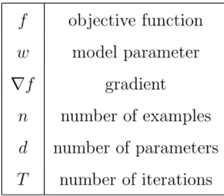
Figure 1: Comparison of three methods: SGD, SVRG, SGDSVRG on MNIST dataset.
2.5.1 Shared-Memory Architecture
We conduct experiments on a machine which has 2 sockets, and each socket has 18 cores. OpenMP library 1 is used to handle shared-memory parallelism. We consider the multi-class classification task on MNIST dataset [57], and use 10,000 training samples and 2,000 testing samples in the experiment. Each image sample is a vector of 784 pixels. We construct a toy three-layer neural network (784 ×100 ×10), where ReLU activation function is used in the hidden layer. We train this neural network with softmax loss function, and `2 regularization with weight C = 10−3. We set mini-batch size |It| = 10, and inner iteration length m= 1,000. Updating only one component ofw in each iteration is too time consuming, therefore we randomly select and update 1,000 components.
We compare following three methods in the experiment:
• SGD: We implement stochastic gradient descent (SGD) algorithm and train with the best tuned learning rate. In our experiment, we use polynomial learning rate η= (1+s)α β,
where α is tuned from {1e−2,5e−2,1e−3,5e−3,1e−4,5e−4,1e−5,5e−5}, β is tuned from in
{0,0.1,0.2, ...,1} and s denotes the epoch number.
• SVRG: We implement our Shared-AsySVRG method and train with the best tuned constant learning rate α.
Time (seconds) ×104 0 2 4 6 8 10 12 14 Training loss 0 0.2 0.4 0.6 0.8 1 1 thread 4 threads 8 threads 16 threads 24 threads 32 threads (a) Time (seconds) ×104 0 2 4 6 8 10 12 14 Testing error 0 0.1 0.2 0.3 0.4 0.5 0.6 0.7 0.8 0.9 1 1 thread 4 threads 8 threads 16 threads 24 threads 32 threads (b) Number of Threads 1 4 8 16 24 32 Speedup 0 5 10 15 20 25 30 35 Ideal Ours (c)
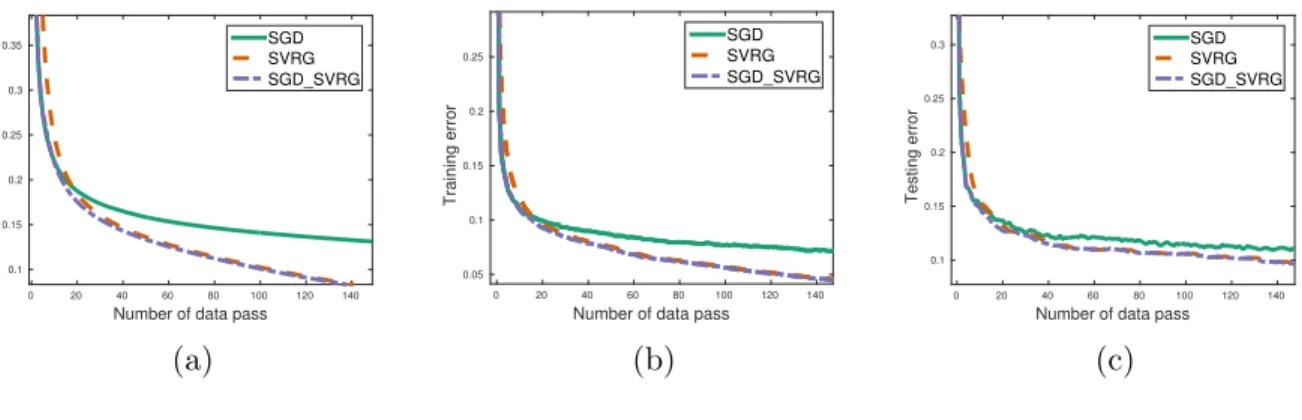
Figure 2: Speedup of Shared-AsySVRG on a machine with different number of threads from 1 to 32.
Number of data pass 0 5 10 15 20 25 Training loss 0.2 0.3 0.4 0.5 0.6 0.7 SGD SVRG SGD_SVRG (a)
Number of data pass
0 5 10 15 20 25 Training error 0.1 0.15 0.2 0.25 0.3 0.35 0.4 0.45 0.5 SGD SVRG SGD_SVRG (b)
Number of data pass
0 5 10 15 20 25 Testing error 0.2 0.25 0.3 0.35 0.4 0.45 0.5 0.55 SGD SVRG SGD_SVRG (c)
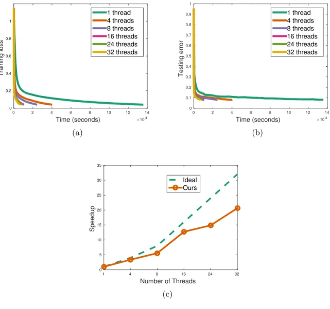
Figure 3: Comparison of three methods: SGD, SVRG, SGDSVRG on CIFAR-10.
• SGD SVRG: SVRG method is sensitive to initial point, and it is slower than SGD at first few iterations. Thus, we apply Shared-AsySVRG on a pre-trained model learned by SGD. In the experiment, we use a pre-trained model after running 10 epochs of SGD method.
We evaluate three compared methods on MNIST dataset, and each method trains with the best tuned learning rate. Figure 1 shows the convergence of each method with respect to different criterion: loss function value on training dataset, training error, and testing error. Figure 1a shows the curves of training loss function value, it is clear that SGD method converges faster than SVRG method in the first 20 iterations, and after that, SVRG method outperforms SGD. SGD SVRG method initializes with a pre-trained model, and it has the best performance. Figure 1b and Figure 1c present the performance of each method on training error and testing error respectively. We can conclude that SVRG and SGD SVRG method have better performance on the long run, and SGD SVRG method has the fastest convergence.
To demonstrate that our proposed Shared-AsySVRG method has linear speedup when we increase the number of workers, we also evaluate Shared-AsySVRG with different number of threads, and Figure 2 presents the result of our experiment. In Figure 2a, all curves are reaching the similar training loss value. As we can see, the more threads we use in the
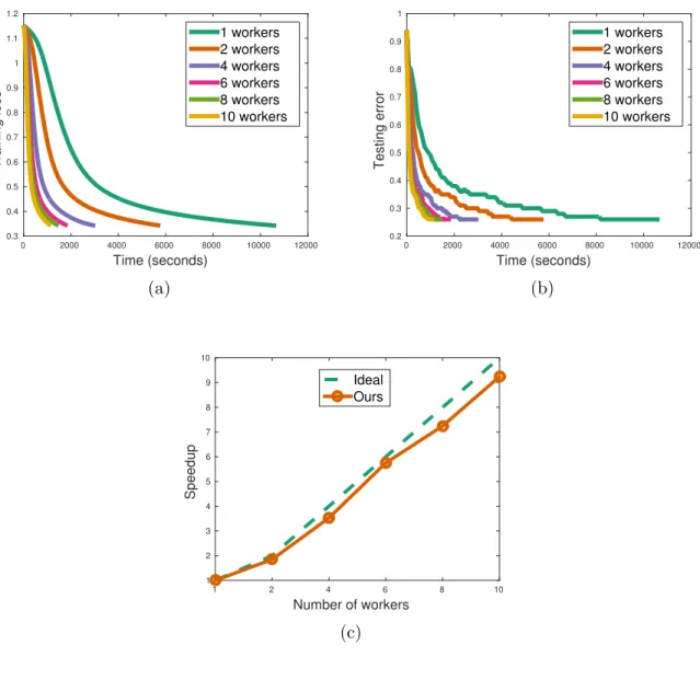
Time (seconds) 0 2000 4000 6000 8000 10000 12000 Training loss 0.3 0.4 0.5 0.6 0.7 0.8 0.9 1 1.1 1.2 1 workers 2 workers 4 workers 6 workers 8 workers 10 workers (a) Time (seconds) 0 2000 4000 6000 8000 10000 12000 Testing error 0.2 0.3 0.4 0.5 0.6 0.7 0.8 0.9 1 1 workers 2 workers 4 workers 6 workers 8 workers 10 workers (b) Number of workers 1 2 4 6 8 10 Speedup 1 2 3 4 5 6 7 8 9 10 Ideal Ours (c)
computation, the less time we need to achieve a similar accuracy. This result is reasonable, because when we distribute the whole work to multiple workers, each worker focuses on its own subset independently and parallelly. The ideal result of parallel computation is linear speedup, namely if we use K threads, its running time should be K1 of the time when we just use a single thread. Figure 2c shows the ideal speedup and actual speedup in our experiment. We can find out that a nearly linear speedup is accessible when we increase the thread number. When the number of threads exceeds a threshold, performance will degrade. These findings in the experiment are compatible with our theoretical analysis.
2.5.2 Distributed-Memory Architecture
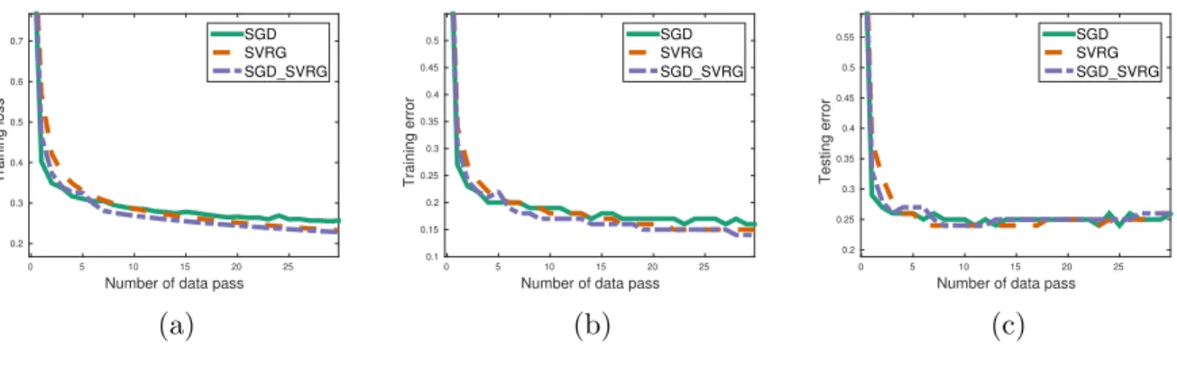
We conduct distributed-memory architecture experiment on AWS platform2, and each node is a t2.micro instance with one virtual CPU. Each server and worker takes a single node. The point to point communication between server and workers are handled by MPICH library3. We use CIFAR-10 dataset [53] in the experiment, and this dataset has 10 classes of color image of size 32×32×3. We use 20,000 samples as training data and 4,000 samples as testing data. We use a pre-trained CNN model in TensorFlow tutorial [1], and extract features from second fully connected layer. Thus, each sample is a vector of size 384. We construct a three-layer fully connected neural network (384×50×10). In the hidden layer, we use ReLU activation function. We train this model with softmax loss, and `2 regularization with weight C = 1e−4. In this experiment, mini-batch size |It| = 10, and the inner loop length m = 2,000. We use the same compared methods as in the last section, except that SGD SVRG method is initialized with parameters learned after 1 epoch of SGD.
Performances of all three methods are presented in Figure 3. Curves in Figure 3a show that SGD is the fastest method in the first few iterations, after that, SVRG-based method will outperform it. It is obvious that SGD SVRG has better convergence rate than SVRG method. We can also draw a similar conclusion from Figure 3b. In Figure 3c, it shows that the test error performance of three compared methods are comparable. We also test our Distributed-AsySVRG method with different number of workers, and Figure 4 illustrates
2https://aws.amazon.com/ 3http://www.mpich.org/
the results of our experiment. It is easy to know that when the number of workers increases, our method has a near linear speedup.
3.0 Asynchronous Dual Free Stochastic Dual Coordinate Ascent for Distributed Data Mining
3.1 Motivation
In this chapter, we consider solving the `2-norm regularized empirical loss minimiza-tion problem which is arising ubiquitously in supervised machine learning and data mining problems: min w∈Rd P(w) := min w∈Rd 1 n n X i=1 φi(w) + λ 2kwk 2 2. (3.1) We let f(w) = 1 n Pn i=1φi(w) and w ∈ R
d be the linear predictor to be optimized. There are many applications falling into this formulation, such as classification, regression, and principal component analysis (PCA). In classification, given featuresxi ∈Rdand labelsyi ∈
{1,−1}, we obtain Support Vector Machine (SVM) when we letφi(w) = max{0,1−yixTi w}. In regression, given featuresxi ∈Rdand responseyi ∈R, we have Ridge Regression problem if φi(w) = (yi −xTi w)2. Recently, [23, 5] showed that the problem of PCA can be solved through convex optimization. SupposingC = n1 Pn
i=1xix T
i be normalized covariance matrix, [23] showed that approximating the principle component of A is equivalent to minimizing
f(w) = 12wT(µI −C)w−bTw given µ > 0 and b ∈ Rd. Defining φi(w) = 1 2w
T((µ− λ 2)I −
xixTi )w−bTwandµ > σ1(C) +λ2 whereσ1(C) denotes the largest singular value ofC, it also falls into problem (3.1). In this case,f(w) is convex while eachφi(w) is probably non-convex. Distributed machine learning and data mining methods are required to solve the problem (3.1) when the data are distributed over multiple machines. In [43], the authors proposed communication-efficient distributed dual coordinate ascent (CoCoA) for primal-dual dis-tributed optimization. In each iteration, the CoCoA framework allows workers to optimize subproblems independently at first. After that, it calls “Reduce” operation to collect local solution from all workers, and updates global variable and broadcasts the up-to-date global variable to workers in the end. It uses stochastic dual coordinate ascent (SDCA) as the local solver which is one of the most successful methods proposed for solving the problem (3.1)
[36, 91]. In [92], the authors proved that SDCA has linear convergence if the convex func-tionφi(w) is smooth, which is much faster than stochastic gradient descent (SGD). [102, 97] also proposed distributed SDCA and analyzed the tradeoff between computation and com-munication. [66, 65] accelerated the CoCoA by allowing for more aggressive updates, and proved that CoCoA has linear primal-dual convergence for the smooth convex problem and sublinear convergence for the non-smooth convex problem. However, there are two issues for these primal-dual distributed methods. Firstly, all of them use SDCA as the local solver. SDCA is not applicable when the dual problem is unknown, e.g. φi is non-convex. There-fore, the applications of these primal-dual distributed methods are limited. Secondly, all of these methods assume that the workers have similar computing speed, which is not true in practice. Straggler problem is an unavoidable practical issue in the distributed data mining. Thus, the computing time of CoCoA and distributed SDCA is dependent on the slowest worker. Even if there is only one bad worker, they will work far slower than expectation.
In [89, 90], the authors proposed dual free stochastic dual coordinate ascent (dfSDCA). It was proved to admit similar convergence rate to SDCA while it did not rely on duality at all. However there is no distributed machine learning method using dfSDCA, and its convergence analysis is still unknown yet.
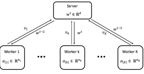
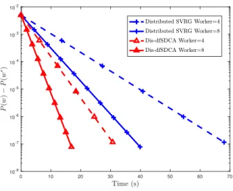
In this chapter, we solve the above two challenging issues in previous primal-dual dis-tributed machine learning methods by proposing novel Disdis-tributed Dual Free Stochastic Dual Coordinate Ascent (dfSDCA). We use dfSDCA as the local solver such that Dis-dfSDCA can be applied to the non-convex problem easily. We alleviate the effect of straggler problem by allowing asynchronous communication between server and workers. As shown in Figure 5, the server does not wait and workers may store the stale global variable in the local. In iteration t, the server receives gradient message vk from worker k, and sends the up-to-datewtback to the worker k. Global variables in other workers are stale. For example worker 1 andK store stale global variables wt−2 and wt−5 respectively. We also analyze the
Figure 5: Distributed asynchronous dual free stochastic dual coordinate ascent for parameter server framework.
3.2 Preliminaries
To optimize the primal problem (3.1), we often derive and optimize its dual problem alternatively: max α∈Rn D(α) := max α∈Rn 1 n n X i=1 −φ∗i(−αi)− λ 2k 1 λnAαk 2 2, (3.2)
where φ∗i is the convex conjugate function to φi, A = [x1, x2, ...xn] ∈ Rd×n denotes data matrix and α ∈ Rn denotes dual variable. We can use stochastic gradient descent (SGD) to optimize primal problem (3.1), however, there are always two issues: (1) SGD is too aggressive at the beginning of the optimization; (2) it does not have a clear stopping criterion. One of the biggest advantages of optimizing the dual problem is that we can keep tracking the duality gap G(α) to monitor the progress of optimization. Duality gap is defined as:
G(α) =P(w(α))−D(α), whereP(w(α)) andD(α) denote objective values of primal problem and dual problem respectively. If w∗ is the optimal solution of primal problem (3.1) and α∗
is the optimal solution of dual problem (3.2), the primal-dual relation always holds that:
w∗ =w(α∗) = 1
λnAα
∗
Algorithm 4 SDCA
1: Initialize α0 and w0 =w(α0);
2: for t = 0,1,2, . . . , T −1 do
3: Randomly sample i from{1,2, ..., n};
4: Find ∆αi to maximize the subproblem (3.4);
5: Update dual variable α through:
αt+1 ←αt+ ∆α iei;
6: Update primal variable w through:
wt+1 ←wt+ λn1 ∆αixi;
7: end for
3.2.1 Stochastic Dual Coordinate Ascent
In [92], the authors proposed stochastic dual coordinate ascent (SDCA) to optimize the dual problem (3.2). The pseudocode of SDCA is presented in Algorithm 4. In iteration t, given samplei and other dual variables αj6=i fixed, we maximize the following subproblem:
max ∆αi∈R −1 nφ ∗ i(−(α t i + ∆αi))− λ 2kw t+ 1 λn∆αixik 2 2, (3.4)
ei denotes coordinate vector of size n, where element i is 1 and other elements are 0. In their chapter, the authors proved that SDCA admits linear convergence rate for smooth loss, which is much faster than stochastic gradient descent (SGD). An accelerated SDCA was also proposed in [91]. However, SDCA is not applicable when it is difficult to derive the dual problem, e.g. φi are non-convex.
3.2.2 Dual Free Stochastic Dual Coordinate Ascent
Algorithm 5 Dual Free SDCA
1: Initialize dual variable α0 = (α00, ..., αn0) where ∀i, α0
i ∈Rd, primal variable w0 =w(α0);
2: for t = 0,1,2, . . . , T −1 do
3: Randomly sample i from{1,2, ..., n};
4: Compute dual residue κthrough:
κ← ∇φi(wt) +αti;
5: Update dual variable αi through:
αt+1i ←αti −ηλnκ;
6: Update primal variable w through:
wt+1 ←wt−ηκ;
7: end for
of dfSDCA is that it is space-consuming to store α, whose space complexity O(nd). We can reduce it to O(n) if ∇φi(w) can be written as ∇φi(xTi w)xi. In [31], the authors accelerated dfSDCA by using non-uniform sampling strategy in each iteration and proved that it admits faster convergence.
3.3 Distributed Asynchronous Dual Free Stochastic Dual Coordinate Ascent
In this section, we propose Distributed Asynchronous Dual Free Stochastic Coordinate Ascent (Dis-dfSDCA) for distributed optimization. Dis-dfSDCA fits for any parameter server framework, where the star-shape network is used. We assume that there arensamples in the dataset, and they are evenly distributed over K workers. In workerk, there arenk samples. It is satisfied that n =PK
k=1nk. Different from sequential dfSDCA, we split the update of dual variable and primal variable into different nodes. The pseudocodes of Dis-dfSDCA for server node and worker nodes are presented in Algorithm 10 and Algorithm 7 respectively.
Algorithm 6 Dis-dfSDCA (Server) Initializew∈Rd, η
for s= 0,1, ..., S−1 do for t= 0,1, ..., T −1 do
Receive gradient message vs,t=v
k from workerk; Update global variable ws+1,t+1 through:
ws,t+1 ←ws,t−ηvs,t; Send ws,t+1 back to worker k ; end for
ws+1,0 =ws,T
Broadcast the up-to-date global variablews+1,0 to all workers. end for
3.3.1 Update Global Variable on Server
The up-to-date global variable w ∈ Rd is stored and updated on the server. Initially,
w is set to be vector zero. At the beginning of each iteration, the server receives gradient message vk from arbitrary worker k and let vt = vk. Then it updates the global variable through:
ws,t+1 =ws,t−ηvt. (3.5)
Finally, it sends the up-to-date global variable back to the workerkfor further computation. Asynchronous method is robust to straggler problem because it allows for updating the global variable when receiving from only one worker. However, if thewin the worker is too stale, it may lead the algorithm to diverge. Therefore, we induce two loops in our algorithm. Server broadcasts the latest global variablewto all workers after everyT iterations. In this way, we
Algorithm 7 Dis-dfSDCA (Worker k) Initializeα[k]∈Rd×nk,η,H
repeat
Receive global variable ws,d(t) from server; Initialize gradient message: vk←0;
Randomly select samples It from{1,· · ·, nk}where |It|=H; for samplei in It do
Compute dual residue κ through:
κ← ∇φi(ws,d(t)) +αi;
Update local dual variable αi through:
αi ←αi−ηλnκ;
Update gradient message vk through:
vk←vk+κ; end for
Send gradient message vk to server; untilTermination
rate by a constant factor. Our Algorithm 6 can also be extended to the accelerated version easily. In this chapter, we only consider the vanilla version and analyze the convergence rate of our algorithm.
3.3.2 Update Local Variable on Worker
In the distributed optimization, workers are responsible for the gradient computation which is the main workload during the optimization. We take arbitrary worker k as an example. Dual variable α[k] ∈ Rnk is only stored and updated in the worker k, each αi is corresponding to samplei. Initially, local variableα[k]is set to be vector zero. After receiving stale global variable ws,d(t) ∈Rd from the server, workerk computes the dual residue κ and updates local variableαi and gradient messagevk forH iterations. SamplesIt are randomly selected in the local dataset, and we set|It|=H. In each iteration, workerkselects a sample
i randomly and computes the dual residue κ for coordinate i of the dual variable through the following function:
κ=∇φi(ws,d(t)) +αi. (3.6)
Dual residue can also be viewed as the gradient in Stochastic Gradient Descent. When we obtain optimal dual variable α∗ and primal variable w∗, κ should be 0. Therefore, it is satisfied that α∗i = −∇φi(w∗). Then worker k updates local dual variable αi and gradient message vk separately through:
αi = αi−ηλnκ, i∈It (3.7)
vk = vk+κ. (3.8)
Because there is only one αi in the cluster, it is always up-to-date. After H iterations, the worker k sends gradient message vk to the server. From the update rule in our algorithm, it is easy to know that the well-known primal-dual relation in the equation (3.3) is always satisfied. The pseudocode of Dis-dfSDCA in worker node k is described in Algorithm 7.
In Algorithm 7, we use vanilla dfSDCA in the worker which samples with uniform distri-bution. There are also other sampling techniques proposed to accelerate dfSDCA. As per the sampling strategy in [89, 31, 90, 14], there are three options: uniform sampling, importance sampling, and adaptive sampling. In importance sampling strategy [90], it first computes the fixed probability distribution pi using smoothness parameter of each function φi, then selects samples following this probability. In adaptive sampling strategy [31], it computes the adaptive probability distribution pi using dual residueκ for each sample every iteration,
3.4 Convergence Analysis
In this section, we provide the theoretical convergence analysis of Dis-dfSDCA. For the case of convex lossesφi, we prove that Dis-dfSDCA admits linear convergence rate. If losses
φi are non-convex, we also prove linear convergence rate as long as the sum-of-non-convex objectives f is convex.
We make the following assumptions for the primal problem (3.1) for further analysis. All of them are common assumptions in the theoretical analysis for the asynchronous stochastic methods.
Assumption 3.4.1(Lipschitz Constant). We assume∇φi is Lipschitz continuous, and there
is Lipschitz constant L such that ∀x, y ∈Rd:
k∇φi(x)− ∇φi(y)k2 ≤Lkx−yk2. (3.9)
We can also know that P is (L+λ)-smooth:
k∇P(x)− ∇P(y)k2 ≤(L+λ)kx−yk2. (3.10)
Assumption 3.4.2 (Maximum Time Delay). We assume that the maximum time delay of the global variable in each worker is upper bounded by τ, such that:
d(t)≥t−τ. (3.11)
τ is relevant to the number of workersK in the system. We can also control τ through inner iteration T in our algorithm.
3.4.1 Convex Case
In this section, we assume that the losses φi are convex, and prove that our method admits linear convergence.
Assumption 3.4.3 (Convexity). We assume losses φi are convex, such that ∀x, y ∈Rd:
φi(x)≥φi(y) +∇φi(y)T(x−y). (3.12) In our algorithm, dual variables α[1], ..., α[K] are stored in local workers. For worker k, there is no update of α[k] from d(t) to t. Therefore, it is always true that α
s,t [k]= α
s,d(t) [k] . For brevity, we write vs,t, ws,t and αs,t as vt, wt and αt. According to our algorithm, we know that: vt =X i∈It ∇φi(wd(t)) +α d(t) i =X i∈It vit. (3.13)
where |It| = H and E[vit] = ∇P(wd(t)). In our analysis, we also assume that there are no duplicate samples in It. To analyze the convergence rate of our method, we need to prove the following Lemma 3.4.1 at first.
Lemma 3.4.1. Let w∗ be the global solution of P(w), and α∗i = −∇φi(w∗). Following the
proof in [89], we define At and Bt as follows:
At = Ekαti−α ∗ ik 2 , (3.14) Bt = Ekwt−w∗k2. (3.15)
According to our algorithm, we can prove that At+1 and Bt+1 are upper bounded:
E[At+1−At] ≤ −ηλHEkαit−α ∗ ik 2−2ηHLλ2 Ekwt−w∗k2 +4ηλHL P(xt)−P(w∗)−ηλ(1−ηλn)Ekvtk2 t−1 X
Theorem 3.4.1. Suppose losses φi are convex and ∇φi are Lipschitz continuous. Let w∗ be
the optimal solution to P(w), and α∗i =−∇φi(w∗). Define Ct = 2λL1 At+Bt. We can prove
that as long as:
η≤ 1
4HLτ2 +λn+ 2L, (3.18)
the following inequality holds:
E[CT]≤(1−ηλH)E[C0]. (3.19)
Proof of Theorem 3.4.1: SubstitutingAt+1 and Bt+1 according to Lemma 3.4.1, the follow-ing inequality holds that:
E[Ct+1] = 1 2λLAt+1+Bt+1 ≤ (1−ηλH)E[Ct] + 2τ HLη3 t−1 X j=d(t) Ekvjk2 + η2λn 2L +η 2− η 2L Ekvtk2. (3.20) Adding the above inequality from t= 0 to t=T −1, we have:
T−1 X t=0 E[Ct+1]≤ T−1 X t=0 (1−ηλH)E[Ct] + 2Hτ2η2+ η 2λn 2L +η 2− η 2L T−1 X t=0 Ekvtk2, (3.21)
where the inequality follows from Assumption 3.4.2 andηL ≤1. If 2Hη2τ2+η2λn
2L +η 2− η 2L ≤ 0, such that: η≤ 1 4HLτ2 +λn+ 2L, (3.22)
we have the following inequality: T−1 X t=0 E[Ct+1] ≤ T−1 X t=0 (1−ηλH)E[Ct] ≤ T−1 X t=1 E[Ct] + (1−ηλH)C0. (3.23)