UNIVERSITY OF
ROCHESTER
Learning under Ambiguity
Epstein, Larry, and Martin Schneider Working Paper No. 527
LEARNING UNDER AMBIGUITY
∗
Larry G. Epstein
Martin Schneider
March 25, 2006
Abstract
This paper considers learning when the distinction between risk and ambiguity matters. It first describes thought experiments, dynamic variants of those pro-vided by Ellsberg, that highlight a sense in which the Bayesian learning model is extreme - it models agents who are implausibly ambitious about what they can learn in complicated environments. The paper then provides a generalization of the Bayesian model that accommodates the intuitive choices in the thought ex-periments. In particular, the model allows decision-makers’ confidence about the environment to change — along with beliefs — as they learn. A calibrated portfolio choice application shows how this property induces a trend towards more stock market participation and investment.
1
INTRODUCTION
Models of learning typically assume that agents assign (subjective) probabilities to all relevant uncertain events. As a result, they leave no role for confidence in probability assessments; in particular, the degree of confidence does not affect behavior. Thus, for example, agents do not distinguish between risky situations, where the odds are objectively known, and ambiguous situations, where they may have little information and hence also little confidence regarding the true odds. The Ellsberg Paradox has shown that this distinction is behaviorally meaningful in a static context: people treat ambiguous bets differently from risky ones. Importantly, the lack of confidence reflected
∗Epstein: Department of Economics, U. Rochester, [email protected]; Schneider:
Depart-ment of Economics, NYU, and Federal Reserve Bank of Minneapolis, [email protected]. Epstein acknowl-edges financial support from NSF (grant SES-9972442). We are grateful to Hal Cole, Mark Grinblatt, Narayana Kocherlakota, Mark Machina, Massimo Marinacci, Monika Piazzesi, Bryan Routledge, Pietro Veronesi and seminar participants at Berkeley, Carnegie-Mellon, Chicago, Davis, the Federal Reserve Bank of Atlanta, Iowa, the NBER Summer Institute, NYU, Northwestern, Rice, Rochester, Stanford and Wharton for helpful comments. This paper reflects the views of the authors and not necessarily those of the Federal Reserve Bank of Minneapolis or the Federal Reserve System.
by choices in the Ellsberg Paradox cannot be rationalized by any probability belief. In particular, it is inconsistent with the foundations of Bayesian models of learning.
This paper considers learning when the distinction between risk and ambiguity mat-ters. We assume that decision makers view data as being generated by the same memory-less mechanism in every period. Thisa priori view motivates the exchangeable Bayesian model of learning and is commonly imposed on learners in a wide variety of economic applications. We view our principal contribution as two-fold. First, we describe exam-ples or thought experiments, dynamic variants of those provided by Ellsberg, in which intuitive behavior contradicts the (exchangeable) Bayesian learning model. As in the static setting addressed by the Ellsberg Paradox, an agent may lack confidence in her
initial information about the environment. However, confidence may now change as the
agent learns. The examples reveal also another sense in which the Bayesian model is extreme - it models agents who are very ambitious about what they can learn, even in very complicated environments.
Our second contribution is to provide a generalization of the Bayesian model that accommodates the intuitive choices in the thought experiments. The model describes how the confidence of ambiguity averse decision-makers changes over time. Beliefs and confidence are jointly represented by an evolving set of conditional distributions over future states of the world. This set may shrink over time as agents become more familiar with the environment, but it may also expand if new information is surprising relative to past experience. We argue also that it models agents who take the complexity of their environment seriously and therefore are less ambitious than Bayesians about how much can be learned. Finally, we show that the model is tractable in economic settings by applying it to dynamic portfolio choice.
The Bayesian model of learning about a memoryless mechanism is summarized by a triple (Θ, µ0, ), where Θ is a parameter space, µ0 is a prior over parameters, and is a
likelihood. The parameter space represents features of the data generating mechanism that the decision-maker tries to learn. The prior µ0 represents initial beliefs about para-meters. For a given parameter valueθ ∈Θ, the data are an independent and identically distributed sequence of signals{st}∞t=1, where the distribution of any signalstis described by the probability measure (·|θ) on the period state space St=S. The triple (Θ, µ0, )
is the decision-maker’s theory of how data are generated. This theory incorporates both prior information (throughµ0) and a view of how the signals are related to the underlying
parameter (through ). Beliefs on (payoff-relevant) states are equivalently represented by a probability measureponsequences of signals (that is, onS∞), or by the process{p
t}of one-step-ahead conditionals ofp. The dynamics of Bayesian learning can be summarized by pt ¡ ·|st¢ = Z Θ (· |θ)dµt(θ|s t ), (1) wherest= (s
1, ..., st)denotes the sample history at tand whereµt is the posterior belief aboutθ, derived via Bayes’ Rule.
of recursive multiple-priors utility, a model of utility put forth in Epstein and Wang [10] and axiomatized in Epstein and Schneider [7], that extends Gilboa and Schmeidler’s [12] model of decision making under ambiguity to an intertemporal setting. Under recursive multiple-priors utility, beliefs and confidence are determined by a process {Pt} giving for each time and history aset of one-step-ahead conditionals. Since these sets describe responses to data, they are the natural vehicle for modeling learning. The present paper introduces a structure for the process {Pt} designed to capture learning about a mem-oryless mechanism. The process is constructed from a triple of sets (Θ,M0,L). As in
the Bayesian case, Θis a parameter space. The set of priors M0 represents the agent’s
initial view of these parameters. When M0 is not a singleton, it also captures (lack of)
confidence in the information upon which this initial view is based. Finally, a set of likelihoods L represents the agent’s a priori view of the connection between signals and the true parameter.
The multiplicity of likelihoods and the distinction between Θ and L are central to the way we model an agent who has modest (or realistic) ambitions about what she can learn. The setΘrepresents features of the environment that the agent views as constant over time and that she therefore expects to learn. However, in complicated environments she may be wary of a host of other poorly understood factors that also affect realized signals. They vary over time in a way that she does not understand well enough even to theorize about and therefore she does not try to learn about them. The multiplicity of likelihoods inL captures these factors. Under regularity conditions, we show that beliefs become concentrated on one parameter value inΘ. However, ambiguity need not vanish in the long run, since the time-varying unknown features remain impossible to know even after many observations. Instead, the agent moves towards a state of time-invariant ambiguity, where she has learned all that she can.1
As a concrete illustration, consider independent tosses of a sequence of coins. If the decision-maker perceives the coins to be identical, then after many tosses she will naturally become confident that the observed empirical frequency of heads is close to a “true” frequency of heads that is relevant for forecasting future tosses. Thus she will eventually become confident enough to view the data as an i.i.d. process. This laboratory-style situation is captured by the Bayesian model.2
More generally, suppose that she believes the tosses to be independent, but that she has no reason to be sure that the coins are identical - for example, she might be told the same about each coin but very little (or nothing at all) about each. Then she would plausibly admit the possibility that the coins are not identical. In particular, there is no longer a compelling reason why data in the future should be i.i.d. with frequency of heads equal to the empirical frequency of heads observed in the past. Indeed, in contrast to a Bayesian, she may not even be sure whether the empirical frequencies of the data will
1Existing dynamic applications of ambiguity typically impose time-invariant ambiguity. Our model
makes explicit that this can be justified as the outcome of a learning process. See Epstein and Schneider [8] for further properties of time invariant ambiguity.
2Under regularity conditions, the posteriorµ
tconverges to a Dirac measure onΘ, almost surely under p, the Bayesian’s subjective probability on sequences of data; see Schervish [21].
converge, let alone expect her learning process to settle down at a single i.i.d. process.3
This situation cannot be captured by the exchangeable Bayesian model.4 One can view
our model as an attempt to capture learning in such complicated (or vaguely specified and poorly understood) environments.
To illustrate our model in an economic setting, we study portfolio choice and asset market participation by investors who are ambiguity averse and learn over time about asset returns. Selective participation in asset markets has been shown to be consistent with optimalstatic (or myopic) portfolio choice by ambiguity averse investors (Dow and Werlang [5]). What is new in the present paper is that we solve the — more realistic —
intertemporal problem of an investor who rebalances his portfolio in light of new
infor-mation that affects both beliefs and confidence. A key property of the solution is that an increase in confidence — captured in our model by a posterior set that shrinks over time — induces a quantitatively significant trend towards stock market market participation and investment. This is in contrast to Bayesian studies of estimation risk, which tend to
find small effects of learning on investment.
Another novel feature of the optimal portfolio is that the investment horizon matters for asset allocation because investors hedge exposure to an unknown (ambiguous) factor they are learning about. This hedging of ambiguity is distinct from the familiar hedging demand driven by intertemporal substitution effects stressed by Merton [17]. Indeed, we show that it arises even when preferences over risky payoff streams are logarithmic, so that the traditional hedging demand is zero.
We are aware of only three formal treatments of learning under ambiguity. Mari-nacci [16] studies repeated sampling with replacement from an Ellsberg urn and shows that ambiguity is resolved asymptotically. A primary difference from our model is that Marinacci assumes a single likelihood. The statistical model proposed by Walley [22, pp. 457-72] differs in details from ours, but is in the same spirit; in particular, it also features multiple likelihoods. An important difference, however, is that our model is consistent with a coherent axiomatic theory of dynamic choice between consumption processes. Ac-cordingly, it is readily applicable to economic settings. A similar remark applies to Huber [13], who also points to the desirability of admitting multiple likelihoods and outlines one proposal for doing so.
The paper is organized as follows. Section 2 presents a sequence of thought experi-ments to motivate our model. Section 3 briefly reviews recursive multiple-priors utility and then introduces the learning model. Section 4 establishes properties of learning in the short and long run. The portfolio choice application is described in Section 5. Proofs are collected in the appendix.
3For the exchangeable Bayesian model, convergence of empirical frequencies is a consequence of the
LLN for exchangeable random variables; see Schervish [21].
4If the data are generated by a memoryless mechanism and information about each observation is
a priori the same, the exchangeable model is the only relevant Bayesian model. More complicated Bayesian models that introduce either serial dependence or a dependence of the distribution on calendar time are not applicable.
2
EXAMPLES
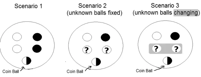
In this section, we consider three related learning scenarios. Each involves urns containing
five balls that are either black or white; Figure 1 illustrates the composition of the urns. However, the scenarios differ in a way intended to illustrate alternative hypotheses about learning in economic environments, and to motivate the main ingredients of our model. In particular, we highlight intuitive behavior that we show later can be accommodated by our learning model but not by the Bayesian model.
Scenario 1: Pure risk
An urn contains five balls. The agent is told that two are black, two are white and that thefifth is either black or white depending on the outcome of the toss of an unbiased coin - the ‘coin ball’ is black if the coin toss produces heads and it is white otherwise. She cannot see the outcome of the coin toss, but she does observe, every period, a black or white ball. Her ex ante view is that these data are generated by sampling with replacement from the given urn. This may be because she is actually doing the sampling, or because she has been told that this is how signals are generated. Alternatively, it may simply reflect her subjective view of the environment. In any case, the obvious version of the Bayesian learning model (1) seems appropriate. In particular, she can be confident of learning the color of the coin ball.
Scenario 2: Ambiguous prior information about a fixed urn
The information provided about the urn is modified to: there is at least one non-coin ball of each color. Thus unlike Scenario 1, no objective probabilities are given for the composition of the urn — there is ambiguity about the number of black non-coin balls. However, signals are again observed in each period, and they are viewed as resulting from sampling with replacement from the given urn. Because the agent views the factors underlying signals, namely the color composition of the urn, as fixed through time, she can hope to learn it. That is, she would try to learn the true composition of the ambiguous urn.
Compare this situation with the purely risky one, Scenario 1 above, assuming the two coin tosses are independent. In particular, consider the choice between betting on drawing black (white) from the risky urn as opposed to the ambiguous one. (Throughout a bet on the color of a ball drawn from an urn is understood to pay one util if the ball has the desired color and zero otherwise.) The Ellsberg Paradox examines this choice prior to any sampling. As recalled in the introduction, the intuitive behavior pointed to by Ellsberg - the preference to bet on drawing black from the risky urn as opposed to the ambiguous one, and a similar preference for white - is inconsistent with a single prior on the composition of the ambiguous urn.
Consider the ranking of bets after some sampling. It is plausible that Ellsberg-type behavior persists in the short run: for any sufficiently short common sample history across the risky and ambiguous urns, a bet on the risky urn should remain preferrable to an analogous bet on the ambiguous urn. At the same time, given the ex ante view that
Figure 1:Urns for Scenarios 1-3.
sampling is from an unchanging urn, it is intuitive that learning should resolve ambiguity
in the long run. Asymptotically the agent should behave as if she knew the fraction
of black balls were equal to their empirical frequency. In the limit, for any common sample history across the two urns, she should be indifferent between betting on the next draw from the risky as opposed to the ambiguous urn. Both Scenarios 1 and 2 are thus conducive to inference and learning because there is one urn withfixed composition. Next we examine learning in a more complex setting where signals are generated by a sequence of urns with time-varying composition.
Scenario 3: Unambiguous prior and changing urns
Signals are generated by successive sampling from asequence of urns, each containing black and white balls. The urns are perceived in the following way: each urn consists of a coin ball and four other balls as above. The coin is tossed once at the start and determines the same color for coin-balls in all urns. However, non-coin balls are replaced every period with a new set of non-coin balls. This task is performed every period by an administrator. It is also known that (i) a new administrator is appointed every period,
(ii) no administrator knows the previous history of urns or draws and (iii) the only restriction on any given administrator is that at least one non-coin ball of each color be placed in the urn.
Ex ante, before any draws are observed, this environment looks the same as Scenario 2: there is one coin ball, there is at least one black and one white non-coin ball, and there are two non-coin balls about which there is no information. The new feature in Scenario 3 is that the non-coin balls change over time in a way that is not well understood. What might an agent now try to learn? Since the coin-ball is fixed across urns and underlies all signals, it still makes sense to try to learn its color. At the same time, learning about the changing sequence of non-coin balls has become more difficult. Compared to Scenario 2, one would thus expect agents to perceive more uncertainty about the overall
proportion of black balls. We now argue that this should lead to different behavior in the two scenarios both in the short run and in the long run.
Begin again by considering betting behavior in the short run, assuming that the coin tosses in Scenarios 2 and 3 are independent. Before any sampling, one should be indifferent between bets in Scenarios 2 and 3, since the two settings area priori identical. However,suppose that one black draw from each urn has been observed and consider bets on the next draw being black. It is intuitive that the agent prefer to bet on black in the
next draw in Scenario 2 rather than on the next draw in Scenario 3. This is because
the observed black draw in Scenario 2 is stronger evidence for the next draw also being black than is the observed black draw in Scenario 3. In Scenario 3, the agent does not understand well the dynamics of the non-coin balls and thus is plausibly concerned that the next urn may contain more white balls than did the first. Of course, she thinks that the next urn may also contain more black balls, but as in the static Ellsberg choice problem, the more pessimistic possibility outweighs the optimistic one. Thus she would rather bet in Scenario 2 where the number of black non-coin balls is perceived not to change between urns.
Turn to behavior in the long run. Scenarios 2 and 3 differ in what qualifies as a reasonable a priori view about the convergence of empirical frequencies. Since the urn in Scenario 2 is essentially fixed, one should be confident that the fraction of black balls drawn converges to some limit. In contrast, nothing in the description of Scenario 3 indicates that such convergence will occur. The sequence of administrators suggests only that the number of black non-coin balls is independent across successive urns. Otherwise, the description of the environment is very much consistent with perpetual change. It is thus reasonable to expect a priori that nothing can be learned about future non-coin balls from sampling. Given how little information is provided about any single urn, the number of non-coin balls should be perceived as ambiguous at all dates. In particular, even after long identical samples from the two scenarios, one would still prefer to bet on the next draw being black from the urns in Scenario 2 rather than in Scenario 3.
Desirable Properties of a Learning Model
To sum up, we would like a model that captures the following intuitive choices between bets in Scenarios 1-3. First, bets on risky urns (Scenario 1) are preferred to bets on ambiguous urns withfixed composition (Scenario 2) in the short run, but not in the long run. In other words, with only ambiguous prior information, Ellsberg type behavior is observed in the short run, but not in the long run. Second, bets on risky urns (Scenario 1) are preferred to bets on ambiguous urns with changing composition (Scenario 3) in both the short and long run. In other words, in a complicated environment with changing urns, Ellsberg type behavior persists. It is clear that the Bayesian model cannot generate these choices, since it never gives rise to Ellsberg-type behavior. Finally, bets on ambiguous urns with fixed composition (Scenario 2) should be preferred to bets on ambiguous urns with changing composition (Scenario 3). This third choice emphasizes that the distinction between ambiguous prior information about a fixed urn and ambiguity perceived about changing urns is behaviorally important.
3
A MODEL OF LEARNING
3.1
Recursive Multiple-Priors
We work with a finite period state space St = S, identical for all times. One element
st ∈S is observed every period. At timet, an agent’s information consists of the history
st = (s
1, ..., st). There is an infinite horizon, so S∞ is the full state space.5 The agent ranks consumption plans c= (ct), where ct is a function of the history st. At any date
t = 0,1, ..., given the history st, the agent’s ordering is represented by a conditional utility functionUt, defined recursively by
Ut(c;st) = min p∈Pt(st)
Ep £u(ct) + βUt+1(c;st, st+1)
¤
, (2)
whereβandusatisfy the usual properties. The set of probability measuresPt(st)models beliefs about the next observationst+1, given the historyst.Such beliefs reflect ambiguity
when Pt(st) is a nonsingleton. We refer to {Pt} as the process of conditional one-step-ahead beliefs. The process of utility functions is determined by specification of{Pt},u(·) andβ, which constitute the primitives of the functional form.
To clarify the connection to the Gilboa-Schmeidler model, it is helpful to rewrite utility using discounted sums. In a Bayesian model, the set of all conditional-one-step-ahead probabilities uniquely determine a probability measure over the full state space. Similarly, the process {Pt} determines a unique set of probability measures P on S∞ satisfying the regularity conditions specified in Epstein and Schneider [7].6 Thus one obtains the following equivalent and explicit formula for utility:
Ut(c;st) = min p∈P E p £Σ s≥tβs−tu(cs) | st ¤ . (3)
This expression shows that each conditional ordering conforms to the multiple-priors model in Gilboa and Schmeidler [12], with the set of priors for time t determined by updating the setP measure-by-measure via Bayes’ Rule.
Axiomatic foundations for recursive multiple-priors utility are provided in Epstein and Schneider [7]. The essential axioms are that conditional orderings(i)satisfy the Gilboa-Schmeidler axioms, (ii) are connected by dynamic consistency, and (iii) do not depend on unrealized parts of the decision tree - utility given the history st, depends only on consumption in states of the world that can still occur. To ensure such dynamic behavior in an application, it is sufficient to specify beliefs directly via a process of one-step-ahead conditionals {Pt}. In the case of learning, this approach has additional appeal: because
5In what follows, measures onS∞are understood to be defined on the productσ-algebra onS∞, and
those on anyStare understood to be defined on the power set ofSt. While our formalism is expressed forSfinite, it can be justified also for suitable metric spacesSbut we ignore the technical details needed to make the sequel rigorous more generally.
6In the infinite horizon case, uniqueness obtains only if P is assumed also to be regular in a sense
defined in Epstein and Schneider [8], generalizing to sets of priors the standard notion of regularity for a single prior.
{Pt} describes how an agent’s view of the next state of the world depends on history, it is a natural vehicle for modeling learning dynamics. The analysis in [7] restricts {Pt} only by technical regularity conditions. We now proceed to add further restrictions to capture how the agent responds to data.
3.2
Learning
Our model of learning applies to situations where a decision-maker holds the a priori view that data are generated by the same memoryless mechanism every period. This a
priori view also motivates the Bayesian model of learning about an underlying parameter
from conditionally i.i.d. signals.
As in the Bayesian model outlined in the introduction, our starting point is again (a
finite period state spaceS and) a parameter spaceΘthat represents features of the data the decision-maker tries to learn. To accommodate ambiguity in initial beliefs about parameters, represent those beliefs by a set M0 of probability measures on Θ. The
size of M0 reflects the decision-maker’s (lack of) confidence in the prior information on
which initial beliefs are based. A technically convenient assumption is thatM0 is weakly
compact;7 this permits us to refer to minima, rather than infima, overM0.
Finally, we adopt a set of likelihoods L - every parameter value θ ∈ Θ is associated with a set of probability measures
L(· |θ) = { (· |θ) : ∈L}.
Each : Θ −→ ∆(S) is a likelihood function, so that θ 7−→ (A | θ) is assumed measurable for everyA⊂S. Another convenient technical condition is thatLis compact when viewed as a subset of(∆(S))Θ (under the product topology). Finally, to avoid the problem of conditioning on zero probability events, assume that each (· |θ) has full support.
Turn to interpretation. The general idea is that the agent perceives the data gener-ating mechanism as having some unknown features, represented by θ, that are common across experiments. Because these features are perceived as common across time or ex-periments, she can try to learn about them. At the same time, she feels there are other factors underlying data, represented by L, that are variable across experiments. It is known that the variable features are determined by a memoryless mechanism — this is why the setL does not depend on history. It is also known that the relative importance of the variable features is the same every period, as in the urn example where there are always four non-coin balls and one coin ball. This is why the set L does not depend on time. However, the factors modeled by the set L are variable across time in a way that the agent does not understand beyond the limitation imposed byL. In particular, at any point in time, any element of L might be relevant for generating the next observation.
7More precisely, measures inM
0 are defined on the implicit and suppressedσ-algebraB associated
with Θ. Take the latter to be the power set whenΘ is finite. The weak topology is that induced by bounded andB-measurable real-valued functions on Θ. M0 is weakly compact iffit is weakly closed.
Accordingly, while she can try to learn the true θ, she has decided that she will not try to (or is not able to) learn more.
Conditional independence implies that past signals st affect beliefs about future sig-nals (such as st+1) only to the extent that they affect beliefs about the parameter. Let
Mt(st), to be described below, denote the set of posterior beliefs aboutθ given that the sample st has been observed. The dynamics of learning can again be summarized by a process of one-step-ahead conditional beliefs. However, in contrast to the Bayesian case (1), there is now a (typically nondegenerate)set assigned to every history:
Pt(st) = ½ pt(·) = Z Θ (· |θ)dµt(θ) :µt∈Mt(st), ∈L ¾ , (4)
or, in convenient notation,
Pt(st) =
Z
Θ
L(· |θ)dMt(θ).
This process enters the specification of recursive multiple priors preferences (2).8 Updating and reevaluation
To complete the description of the model, it remains to describe the evolution of the posterior beliefs Mt. Imagine a decision-maker at time t looking back at the sample
st. In general, she views both her prior information and the sequence of signals as ambiguous. As a result, she will typically entertain a number of different theories about how the sample was generated. A theory is a pair (µ0, t), where µ0 is a prior belief on
Θ and t= ( 1, .., t)∈Lt is asequence of likelihoods. The decision-maker contemplates different sequences t because she is not confident that signals are identically distributed over time.
We allow for different attitude towards past and future signals. On the one hand, L is the set of likelihoods possible in the future. Since the decision-maker has decided she cannot learn the true sequence of likelihoods, it is natural that beliefs about the future be based on the whole set L as in (4). On the other hand, the decision-maker may
reevaluate, with hindsight, her views about what sequence of likelihoods was relevant
for generating data in the past. Such revision is possible because the agent learns more aboutθ and this might make certain theories more or less plausible. For example, some interpretation of the signals, reflected in a certain sequence t= (
1, ..., t), or some prior experience, reflected in a certain prior µ0 ∈ M0, might appear not very relevant if it is
part of a theory that does not explain the data well.
To formalize reevaluation, we need two preliminary steps. First, how well a theory
(µ0, t)explains the data is captured by the (unconditional) data density evaluated at st:
Z
Πtj=1 j(sj|θ)dµ0(θ).
8Given compactness of M
0 and L, one can show that Mt(st) defined below is also compact, and subsequently that eachPt(st)is compact. This justifies the use of minima in (2).
Here conditional independence implies that the conditional distribution givenθ is simply the product of the likelihoods j. Prior information is taken into account by integrating out the parameter using the prior µ0. The higher the data density, the better is the
observed sample st explained by the theory (µ
0, t). Second, let µt(· ;st, µ0, t) denote
the posterior derived from the theory (µ0, t) by Bayes’ Rule given the data st. This posterior can be calculated recursively by Bayes’ Rule, taking into account time variation in likelihoods: dµt¡· ;st, µ0, t¢= R t(st | ·) Θ t(st|θ 0)dµ t−1(θ0;st−1, µ0, t−1) dµt−1(· ;st, µ0, t−1). (5)
Reevaluation takes the form of a likelihood-ratio test. The decision-maker discards all theories (µ0, t) that do not pass a likelihood-ratio test against an alternative theory that puts maximum likelihood on the sample. Posteriors are formed only for theories that pass the test. Thus posteriors are given by
Mαt(s t) = {µt¡st;µ0, t¢: µ0 ∈M, t∈Lt, (6) Z Πtj=1 j(sj|θ)dµ0(θ)≥α max ˜ µ0∈M0 ˜t∈Lt Z Πtj=1˜j(sj|θ)dµ˜0}.
Here α is a parameter, 0< α≤ 1, that governs the extent to which the decision-maker is willing to reevaluate her views about how past data were generated in the light of new sample information. The likelihood-ratio test is more stringent and the set of posteriors smaller, the greater is α. In the extreme case α = 1, only parameters that achieve the maximum likelihood are permitted. If the maximum likelihood estimator is unique, ambiguity about parameters is resolved as soon as the first signal is observed. More generally, we have that α > α0 implies Mα
t ⊂ Mα
0
t . It is important that the test is done after every history. In particular, a theory that was disregarded at time t might look more plausible at a later time and posteriors based on it may again be taken into account.
In summary, our model of learning about an ambiguous memoryless mechanism is given by the tuple (Θ,M0,L, α). As described, the latter induces, or represents, the
process {Pt} of one-step-ahead conditionals via
Pt(st) =
Z
Θ L
(· |θ)dMαt(θ),
where Mα
t is given by (6). The model reduces to the Bayesian model when both the set of priors and the set of likelihoods have only a single element.
Another important special case occurs if M0 consists of several Dirac measures on
the parameter space in which case there is a simple interpretation of the updating rule:
Mα
t contains all ˜θ’s such that the hypothesis θ = ˜θ is not rejected by an asymptotic likelihood ratio test performed with the given sample, where the critical value of the
discarded or added to the set, and Pt varies over time. The Dirac priors specification is convenient for applications — it will be used in our portfolio choice example below. Indeed, one may wonder whether there is a need for non-Dirac priors at all. However, more general priors provide a useful way to incorporate objective probabilities, as illustrated by the scenarios in Section 2.9
3.3
Scenarios Revisited
We now describe how we would model the three scenarios of Section 2 and we show that our setup can accommodate the intuitive behavior described there. The results here clarify the role of multiple priors and multiple likelihoods, but are essentially independent of the revaluation parameterα. We return to the role ofαin Section 4, where we consider the evolution of beliefs in the context of Scenario 3.
Scenarios 1 & 2: For both scenarios, specify S ={B, W} and Θ=©5n : n= 1,2,3,4ª. The state s corresponds to the color of a drawn ball, and θ indicates the proportion of black balls (coin or non-coin). For scenario 1, assume that there is a single prior with µ(θ) = 13 for θ = 25,53 or 45 and define the single likelihood by (B |θ) = θ. For scenario 2, specify a representation(Θ,M0,L, α)by settingL={ },fixing a revaluation
parameter α and defining the set M0 of priors on Θ as follows. Let P ⊂ ∆({1,2,3})
denote beliefs about the number of black non-coin balls. Since the coin-ball and other colors are independent, each prior µ0 should have the form
µp0(θ) = 12p(5θ−1) + 12p(5θ) (7) for some p∈P. Thus let M0 ={µp0 :p∈P}.
This setup captures Ellsberg-type behavior in the short run, because the set of one-step-ahead probabilities for the next draw is nondegenerate. For example, a bet on black in Scenario 2 would be evaluated under a prior that puts the lowest possible conditional probability on a black draw, and similarly for white. As a result, either bet in Scenario 2 will be inferior to its counterpart in Scenario 1. In addition, keeping the history of draws the same across scenarios, any difference in utility would become smaller and smaller over time. With a single likelihood, it is easy to verify that the posteriors derived from M0
become more similar over time and eventually become concentrated on a single parameter value. Ambiguity is thus resolved in the long run.
Scenario 3. A natural parameter space here is Θ = {B, W}, corresponding to the two
possible colors of the coin-ball. There is a single prior µ0 — the
¡1 2, 1 2 ¢ prior on Θ cor-responding to the toss of the unbiased coin. Ambiguity perceived about the changing non-coin balls is captured by a nondegenerate set of likelihoods, specified as follows. Let
P ⊂ ∆({1,2,3}) denote beliefs about the number of black non-coin balls, where P is the same set used in Scenario 2. Since thefirst urns in the two scenarios are identical, it
9Another example is in Epstein and Schneider [9], where a representation with a single prior and
α= 0 is used to model the distinction between tangible (well-measured, probabilistic) and intangible (ambiguous) information.
is natural to use the same set P to describe beliefs about them. Moreover, though the urns differ along the sequence in Scenario 3, successive urns are indistinguishable, which explains whyP can be used also to describe the second urn in the present scenario. Each
p inP suggests one likelihood function via
p(B |B) = Σλ p(λ) + 1 5 , p(B |W) = Σλ p(λ) 5 . (8) Finally, let10 L={ p : p∈P}. (9)
Our model of Scenario 3 also leads to a nondegenerate set of one-step-ahead condi-tionals in the short run. The difference from Scenario 2 is that ambiguity enters through beliefs about signals, captured by multiple likelihoods, rather than through multiple priors on Θ. The multiplicity of likelihoods also implies directly that ambiguity never vanishes. Indeed, a bet on black in Scenario 3 will always be evaluated under a likelihood that puts the lowest possible conditional probability on a black draw, and similarly for white. Either bet in Scenario 3 will thus be inferior to its counterpart in Scenario 1, even in the long run.
Focus now on the other choice described above - given that one black ball has been drawn, would you rather bet on the next draw being black in Scenario 2 or in Scenario 3? This question highlights one difference between learning in simple settings (Scenario 2) as opposed to complex ones (Scenario 3), and thus demonstrates the key role played
by multiple-likelihoods. We argued above that it is intuitive that one prefer to bet in
Scenario 2 - the black draw is stronger evidence there for the next draw also being black. The appendix shows that our model predicts these intuitive choices. In particular, it demonstrates that the minimal predictive probability for a black ball conditional on observing a black ball,
min
p P1(B) = ∈L,µmin1∈Mα1(B) Z
Θ
(B |θ)dµ1(θ),
is smaller under Scenario 3 than under Scenario 2. An ambiguity averse agent who ranks bets according to the smallest probability of winning will thus prefer to bet on the urn from Scenario 2.
10Given the symmetry of the environment, a natural candidate forP is
P ={p∈∆({1,2,3}) : Σλp(λ) ∈ [2− ,2 + ]},
where is a parameter,0≤ ≤1.In the special case where = 1, the agent attaches equal weight to all
logically possible urn compositions λ= 1,2,or3. More generally,P incorporates a subjective element into the specification. Just as subjective expected utility theory does not impose connections between the Bayesian prior and objective features of the environment, so too the set of likelihoods is subjective (varies with the agent) and is not uniquely determined by the facts. For example, for <1, the agent attaches more weight to the ‘focal’ likelihood corresponding to λ= 2 as opposed to the more extreme scenariosλ= 1,3.
3.4
Discussion
Two further remarks are in order about the structure of our model and its relationship to the Bayesian model. Consider first the question of foundations. Though recursive multiple-priors is an axiomatic model, we do not have axiomatic foundations for the specialization described here. For the Bayesian model, the de Finetti Theorem shows that the representation (1) is possible if and only if the prior p on S∞ is exchangeable.
We are missing a counterpart of the de Finetti Theorem for our setting. Nevertheless, without discounting the importance of this missing element, we would argue that our model can be justified on the less formal grounds of cognitive plausibility.
Begin with a perspective on the de Finetti Theorem. While de Finetti starts from a prior p on S∞ and the assumption of exchangeability, the usefulness of his theorem
stems in large part from the reverse perspective: it describes a cognitively plausible procedure for a decision-maker to arrive at a priorpand to determine thereby if, indeed, exchangeability is acceptable.11 In some settings, there is a natural pair(Θ, )and, when
Θis simple, forming a prior µ0 overΘis easier than forming one directly overS∞. Thus
the representation (1) can be viewed as providing a procedure for the decision-maker to arrive at the measure p onS∞ to use for decision-making. Moreover, to the extent that (Θ, )is simple and natural given the environment, the procedure is cognitively plausible. In fact, cognitive plausibility is essential to support the typical application of the Bayesian model. After all, a Bayesian modeler must assume a particular parametric specification for (Θ, µ0, ). This amounts, via (1), to assuming a particular prior p for which there is no axiomatic justification. Instead, cognitive plausibility is the only sup-porting argument. However, outside of contrived settings, where the data generating mechanism is simple and transparent, the existence of a cognitively plausible specifi ca-tion of (Θ, µ0, ) is problematic. In particular, the Bayesian model presumes a degree of
confidence on the part of the agent that seems unintuitive in complicated environments. We view enhanced cognitive plausibility as a justification for our model. As illustrated by the examples and the way in which we model them, greater cognitive plausibility is afforded if we allow the decision-maker to have multiple priors on the parameter space
Θ and, more importantly, multiple likelihoods.
A second feature of our model — and one that it shares with the Bayesian approach — is that the decomposition between learnable and unlearnable features of the environment is exogenous. Indeed, the learnable parametersΘand the unlearnable features embodied by a nonsingleton L are given at the outset. We thus do not explain which features the agent tries to learn in any given setting. The same is true in the Bayesian case, where the decomposition is extreme - L is a singleton and the agent tries to identify an i.i.d. process. Thus, while we leave important aspects unmodeled, we do extend the Bayesian model in the direction of permitting more plausible ambitions about what can be learned in complex settings. The Ellsberg-style examples and the portfolio choice application illustrate that natural decompositions may be suggested by descriptions of
the environment.
4
BELIEF DYNAMICS
In this section we illustrate further properties of learning under ambiguity. We first examine the dynamics of beliefs and confidence in the short term, using the example of Scenario 3. We then provide a general result on convergence of the learning process in the long run.
4.1
Inference from Small Samples
As in Section 3.3, take Θ = {B, W}, µ0 = ¡1 2, 1 2 ¢
, and assume further that the agent weighs equally all the logically possible combinations of non-coin balls, that is,Lis given by (8) with
P ={p∈∆({1,2,3}) : Σλp(λ) ∈ [1,3]}
The evolution of the posterior setMα
t in (6) shows how signals tend to induce ambiguity about parameters even where there is no ambiguity ex ante (singletonMα
0). This happens
when the agent views some aspects of the data generating mechanism as too difficult to try to learn, as modeled by a nonsingleton set of likelihoods. More generally, Mαt can expand or shrink depending on the signal realization.
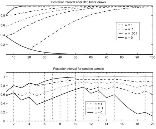
Posterior beliefs can be represented by the intervals
[ min
µt∈Mαt
µt(B), max
µt∈Mαt
µt(B)].
Figure 2 depicts the evolution of beliefs about the coin-ball being black as more balls are drawn. The top panel shows the evolution of the posterior interval for a sequence of draws such that the number of black balls is 35t, for t = 5,10, .... Intervals are shown for α = .1 andα = .001, as well as for α = 0, to illustrate what would happen without revaluation. In addition, a single line is drawn for the case α = 1, where the interval is degenerate. For example, after the first 5 signals, with 3 black balls drawn, the agent withα=.1assigns a posterior probability between.4and.8to the coin ball being black. What happens if the same sample is observed again? Our model captures two effects. First, a larger batch of signals permits more possible interpretations of past signals. For example, having seen ten draws, the agent may believe that all six black draws came aboutalthough each time there were the “most adverse” conditions, that is, all but one non-coin ball was white. This interpretation strongly suggests that the coin ball itself is black. The argument also becomes stronger the more data are available - after only
five draws, the appearance of three black balls under “adverse” conditions is not as remarkable.
Second, even though it is not possible to learn aboutfuturenon-coin balls, past draws are informative about past non-coin balls, not just about the parameter. To illustrate,
suppose 50 draws have been observed, and that 30 of them have been black. Given a theory about the non-coin balls, these observations suggest that the coin ball is more likely to be black than white. At the same time, given a value of the parameter, the observations suggest that more than half of the past urns contained three black non-coin balls. Sensible updating takes the latter feature into account. In our model, this is accommodated by revaluation. The evolution of confidence, measured by the size of the posterior interval, then depends on how much agents reevaluate their views. For an agent with α = .001, the posterior interval expands between t = 5 and t = 20. In this sense, a sample of ten or twenty signals induces more ambiguity than a sample of five. However, reevaluation implies that large enough batches of signals induce less ambiguity than smaller ones.
The lower panel of Figure 2 tracks the evolution of posterior intervals along one particular sample. Black balls were drawn at dates indicated by vertical lines, while white balls were drawn at the other dates. Taking the width of the interval as a measure, the extent of ambiguity is seen to respond to data. In particular, a phase of many black draws (periods 5-11, for example) shrinks the posterior interval, while an ‘outlier’ (the white ball drawn in period 12) makes it expand again. This behavior is reminiscent of the evolution of the Bayesian posterior variance, which is also maximal if the fraction of black balls is one half.
4.2
Beliefs in the Long Run
Turn now to behavior after a large number of draws. As discussed above, our model describes agents who are not sure whether empirical frequencies will converge. Never-theless, it is useful to derive limiting beliefs for the case when such convergence occurs: the limiting beliefs also approximately describe behavior after a large, butfinite, number of draws. Therefore, they characterize behavior in the long run. The limiting result below holds with probability one under a true data-generating process, described by a probability P∗ on S∞. For this process, we require only that the empirical frequencies of each of the finite number of states s ∈ S converge, almost surely under P∗. In what
follows, these limiting frequencies are described by a measure φ on S.
By analogy with the Bayesian case, the natural candidate parameter value on which posteriors might become concentrated maximizes the data density of an infinite sample. With multiple likelihoods, any data density depends on the sequence of likelihoods that is used. In what follows, it is sufficient to focus on sequences such that the same likelihood is used whenever state s is realized. A likelihood sequence can then be represented by a collection ( s)s∈S. Accordingly, define the log data density after maximization over the likelihood sequence by H(θ) := max ( s)s∈S X s∈S φ(s) log s(s|θ). (10) The following result (proven in the appendix) summarizes the behavior of the posterior set in the long run.
10 20 30 40 50 60 70 80 90 100 0.2
0.4 0.6 0.8
Posterior Interval after 3t/5 black draws
α = 1 α = .1 α = .001 α = 0 2 4 6 8 10 12 14 16 18 20 0 0.2 0.4 0.6 0.8 1
Posterior interval for random sample
α = 1
α = .1
α = 0
Figure 2: The Posterior Interval is the range of posterior probability that the coin ball is black,
µt(B). In the top panel, the sample is selected to keep fraction of black balls constant. In the
bottom panel, vertical lines indicate black balls drawn.
Theorem 1 Suppose that Θ is finite and that:
(i) θ∗ = arg maxθH(θ) is a singleton;
(ii) there exists κ >0 such that for every µ0 inMα0,
either µ0(θ∗) = 0 orµ0(θ∗)≥κ,
and µ0(θ∗)>0 for some µ0 inMα
0.
Then every sequence of posteriors from Mαt converges to the Dirac measure δθ∗, almost surely under the true probability P∗, and the convergence is uniform, that is, there is a
set Ω⊂S∞ with P∗(Ω) = 1 and such that for every s∞ in Ω,
µt(θ∗)→1
uniformly over all sequences of posteriors {µt} satisfying µt ∈Mαt (st) for all t.
Condition (i)is an identification condition: it says that there is at least one sequence of likelihoods (that is, the maximum likelihood sequence), such that the sample with empirical frequency measure φ can be used to distinguishθ∗ from any other parameter
value. Condition (ii) is satisfied if every prior inMα
0 assigns positive probability to θ∗
(because Mα
0 is weakly compact). The weaker condition stated accommodates also the
case where all priors are Dirac measures (including specifically the Dirac concentrated at θ∗), as well as the case of a single prior containingθ∗ in its support. (In Scenario 3,
(ii)is satisfied for any set of priors where the probability of a black coin ball is bounded away from zero.)
Under conditions(i)and(ii), and ifΘisfinite, then in the long run only the maximum likelihood sequence is permissible and the set of posteriors converges to a singleton. The agent thus resolves any ambiguity about factors that affect all signals, captured byθ. At the same time, ambiguity about future realizations st does not vanish. Instead, beliefs in the long run become close to L(·|θ∗). The learning process settles down in a state of time-invariant ambiguity.
The asserted uniform convergence is important in order that convergence of beliefs translate into long-run properties of preference. Thus it implies that for the process of one-step-ahead conditionals {Pt} given by (4),
Pt(st) = Z Θ L(· |θ)dMαt(θ), we have min pt∈Pt Z f(st+1)dpt= min µt∈Mαt min ∈L Z Θ ·Z St+1 f(st+1)d (st+1 |θ) ¸ dµt(θ) →min ∈L Z St+1 f(st+1)d (st+1 |θ∗),
for any f : St+1 → R1 describing a one-step-ahead prospect (in utility units). In
par-ticular, this translates directly into the utility of consumption processes for which all uncertainty is resolved next period.
As a concrete example, consider long run beliefs about the urns in Scenario 3. Let
φ∞ denote the limiting frequency of black balls. Suppose also that beliefs are given by (9). Maximizing the data density with respect to the likelihood sequence yields
H(θ) =φ∞max λB log1{θ=B} +λB 5 + (1−φ∞) maxλW log5−1{θ=B}−λW 5 =φ∞log1{θ=B}+ 3 5 + (1−φ∞) log 4−1{θ=B} 5 .
The first term captures all observed black balls and is therefore maximized by assuming
λB = 3 black non-coin balls. Similarly, the likelihood of white draws is maximized by settingλW = 1.It follows that the identification condition is satisfied except in the knife-edge case φ∞ = 12. Moreover, θ∗ = B if and only if φ∞ > 12. Thus the theorem implies that an agent who observes a large number of draws with a fraction of black balls above one half believes it very likely that the color of the coin ball is black. The role of α is
only to regulate the speed of convergence to this limit. This dependence is also apparent from the dynamics of the posterior intervals in Figure 2.
The example also illustrates the role of the likelihood ratio test (6) in ensuring learn-ability of the representation. Suppose that φ∞ = 35. The limiting frequency of 35 black draws could be realized either because there is a black coin ball and on average one half of the non-coin balls were black, or because the coin ball is white and all of the urns contained 3 black non-coin balls. If α were equal to zero, both possibilities would be taken equally seriously and the limiting posterior set would contain Dirac measures that place probability one on either θ = B or θ = W. This pattern is apparent from Figure 2. In contrast, with α > 0, reevaluation eliminates the sequence where all urns contain three black non-coin balls as unlikely.
The set of “true” processes P∗ for which the theorem holds is large. Like a Bayesian
who is sure the data are exchangeable, the agent described by the theorem is convinced that the data generating process is memoryless. As a result, learning is driven only by the empirical frequencies of the one-dimensional events, or subsets of S. Given any process for which those frequencies converge to a given limit, the agent will behave in the same way. Of course, in applications one would typically consider a “truth” that is memoryless. Like the exchangeable Bayesian model, our model is best applied to situations where the agent iscorrect in hisa priori judgement that the data generating process is memoryless. Importantly, a memoryless process for which empirical frequencies converge need not be i.i.d. There exists a large class of serially independent, but nonstationary, processes for which empirical frequencies converge.12 In fact, there is a large class of such processes that cannot be distinguished from an i.i.d. process with distributionφon the basis of any
finite sample. Thus even if they are convinced that the empirical frequencies converge, a concern with ongoing change may lead agents to never be confident that they have identified a “true” i.i.d. data generating process with distributionφ.13
Incomplete learning can occur also in a Bayesian model. For example, if the true data generating measure is not absolutely continuous with respect to an agent’s belief, vio-lating the Blackwell-Dubins [2] conditions, then beliefs may not converge to the truth.14
However, even then the Bayesian agent believes, and behaves as if, they will. In contrast, agents in our model are aware of the presence of hard-to-describe factors that prevent learning and their actions reflect the residual uncertainty.
Incomplete learning occurs also in models with persistent hidden state variables, such as regime switching models. Here learning about the state variable never ceases because agents are sure that the state variable is forever changing. The distribution of these regime changes is known a priori. Agents thus track aknowndata generating process that isnotmemoryless. In contrast, our model applies to memoryless mechanisms and learning is about a fixed true parameter. Nevertheless, because of ambiguity, the agent reaches
12See Nielsen [18] for a broad class of examples.
13As discussed earlier, they may also reach this view because they are not sure whether the empirical
frequencies converge in thefirst place.
14As a simple example, if the parameter governing a memoryless mechanism were outside the support
a state where no further learning is possible although the data generating mechanism is not yet understood completely.
5
DYNAMIC PORTFOLIO CHOICE
In this section, we illustrate the economic consequences of learning under ambiguity by solving the intertemporal portfolio choice problem of an investor who learns about the equity premium. Suppose the investor believes that the equity premium is fixed, but unknown, so that it must be estimated from past returns. Intuitively, one would expect the investor to become more confident in his estimate as more returns are observed. As a result, a given estimate should lead to a higher portfolio weight on stocks, the more data was used to form the estimate.
Bayesian analysis has tried to capture the above intuition by incorporating estimation risk into portfolio problems. One might expect that that the weight on stocks increases as the posterior variance of the equity premium declines through Bayesian learning. However, the effects of estimation risk on portfolio choice tend to be quantitatively small or even zero (see, for example, the survey by Brandt [3]). In fact, in a classic continuous time version of the problem, where an investor with log utility learns about the drift in stock prices, there is no trend in stock investment whatsoever: portfolio weights depend only on the posterior mean, not on the variance (Feldman [11]). The Bayesian investor thus behaves exactly as if the estimate were known to be correct.
Below we revisit the classic log investor problem. We argue that the Bayesian model generates a counterintuitive result because a declining posterior variance does not ad-equately capture changes in confidence. In contrast, when returns are perceived to be ambiguous, an increase in investor confidence — captured in our model by a shrinking set of posterior beliefs — naturally induces a trend toward stock ownership. This trend is quantitatively significant at plausible parameter values. To apply thefinite state frame-work of Section 3.2, we frame-work in a binomial tree setting. However, most results are stated for the continuous time limit of the model. This permits closed-form solutions for beliefs and makes the results more easily comparable to existing work on Bayesian learning. Investor Problem
We measure time in months and assume that there are k trading periods in every month. An investor has access to a riskless asset with constant per period interest rate
Rf = erf/k
and to stocks with uncertain return R(st) = er(st). The state st takes one of two values every period: st ∈ {0,1}. The investor knows the possible (log) return realizationsr(1) =σ/√k andr(0) =−σ/√k, but is not sure about the probabilityπ of the high statest= 1, and hence the monthly mean log return
µ(π) := (2π−1)σ√k.
An investor at the end of monthtplans over the nextT months; she cares about terminal wealth according to the utility function VT (Wt+T) = logWt+T. She may rebalance her
portfolio in every trading period betweentandT. At time t,she knows that rebalancing may be optimal in the future — for example, if learning changes beliefs and confidence — and thus takes the prospect of future learning and rebalancing into account when choosing a portfolio att. We are interested in how the optimal portfolio weight on stocks changes with calendar timet and the investment horizon T.
While calendar time is measured in months, beliefs and the value function are defined for every trading period. The history of state realizations up to trading periodτ =t+j/k
— the jth trading period in montht+ 1 — can be summarized by the fraction φτ of high states observed up to τ. Given one-step-ahead beliefs Pτ(sτ), the value function of the log investor takes the form Vτ(Wτ, sτ) =hτ(φτ) + logWτ.The process {hτ} solves
hτ(φτ) = maxω τ min pτ∈Pτ(sτ) Epτ £log¡Rf +¡R¡s τ+1/k ¢ −Rf¢ωτ ¢ +hτ+1/k ¡ φτ+1/k¢¤ = min pτ∈Pτ(sτ) max ωτ Epτ £log¡Rf +¡R¡s τ+1/k ¢ −Rf¢ωτ ¢ +ht+1/k ¡ φτ+1/k ¢¤ (11) where we have used the minimax theorem to reverse the order of optimization.
Denote by p∗
t(φt) the minimizing (conditional-one-step-ahead) probability. As k be-comes large, the optimal portfolio weight on stocks at datet converges to
ω∗t = µ(p∗ t(φt)) + 12σ 2 −rf σ2 . (12)
This weight is also optimal in a continuous time problem when cumulative returns follow a geometric Brownian motion with volatilityσ and drift µ(p∗
t(φt)) at datet.15
We calibrate the model to monthly real US stock returns. We would like to compute the optimal portfolio of an investor who has seen a monthly sample of log returns{rτ}
t τ=1
taken from the data. Since agents in the model observe binary returns {R(sτ)} per trading period, we construct a sample of tk realizations of R(sτ) such that the implied empirical distribution of monthly log returns is close to that in the data. Fix σ =
1
√
1219.0%, the sample standard devation of monthly log returns from 1926 to 2004. 16
The sample of states can be summarized by the fraction φt, which we determine by matching the means in the two samples, that isµ(φt) = ¯rt:= 1tΣtj=1rj. Standard results imply that, ask → ∞, the empirical distribution of monthly log returns from the model,
Σk j=1R
¡
st+j/k
¢
converges to a normal distribution with mean¯rtand varianceσ2. We also set the riskless rate constant at 2% per year.
Bayesian Benchmark
As a Bayesian benchmark, we assume that the investor has an improper beta prior over the probability π of the high state, so that the posterior mean ofπ after t months (or tk state realizations) is equal to φt, the maximum likelihood estimator of π. The
15Let cumulative stock returns follow dV(t)
V(t) = µ(t)dt+σdB(t), where B is a standard Brownian
motion. Ifµ(t) =µ(p∗
t(φt)), then (12) is the optimal weight of a log investor at datet.
16We use the monthly NYSE-AMEX return from CRSP, net of monthly CPI inflation for all urban
Bayesian’s probability of a high state next period is then also given by φt. The optimal portfolio weight for large k is given by (12) with µ(p∗
t(φt)) =µ(φt) = ¯rt. This weight — denotedωbayt in what follows — is also optimal for a continuous time investor who learns about the drift of cumulative returns, starting from an improper normal prior.
The benchmark clarifies the limitation of the Bayesian model in capturing confidence. In the binomial tree, the optimal portfolio weight of the log investor depends only on the estimate φt, regardless of how many observations it is based on. Similarly, in the continuous time limit, the optimal portfolio weight depends only on the sample meanr¯t. This happens despite the fact that estimation risk is gradually reduced as the posterior variance — here σ2/t — shrinks. Intuitively, estimation risk perceived by a Bayesian is
second order relative to the risk in unexpected returns. In the continuous time limit, estimation risk vanishes altogether.17
Trends in stock investment can occur in the Bayesian case if the investment horizon
T is long and the coefficient of relative risk aversion is different from one.18 However,
the effect of calendar time on the portfolio weight is then due to intertemporal hedging of future news, as emphasized by Brennan [4]. It does not occur because the resolution of risk makes risk averse agents more confident. Indeed, if the coefficient of relative risk aversion is less than one, learning induces a decreasing trend in the optimal portfolio weight, although the investor is risk averse. Moreover, while high risk aversion can generate an increasing trend, the effect is quantitatively small in our setting, as we show below.
Beliefs under Ambiguity
Beliefs under ambiguity are given by a representation (Θ,M0,L, α). The ambiguity
averse investor perceives the mean monthly log return as θ+λt, where θ ∈ Θ := R is
fixed and can be learned, while λt is driven by many poorly understood factors driving returns and can never be learned. The setL consists of all (· |θ) such that
(1|θ) = 1 2 +
1 2
θ+λ
σ√k, for someλ with |λ| <
¯
λ. (13)
Ifλ >0, returns are ambiguous even conditional on the parameter θandλtparametrizes the likelihood t. For fixed θ and λ, and k large, the implied cumulative stock return process approximates a diffusion with volatilityσ and driftµ( (1|θ)) =θ+λ.
17In discrete time, esimtaion risk would induce a small trend effect. Maintaining a diffuse prior and
normality, the one-period-ahead conditional variance of log returns at datetwould beσ2+σ2/t. With a
period length of one month, the effect of estimation risk becomes a small fraction of the overall perceived variance after only a couple of years.
18It follows from results in Rogers [19] that the optimal weight on stocks for a Bayesian investor with
power utility and coefficient of relative risk aversionγis given by ωt= ¯ rt+12σ2−r γσ2 γt γt+ (γ−1)T.
Thefirst fraction is the “myopic demand” that obtains forT = 0; it depends only on the posterior mean. ForT >0,the second fraction captures intertemoporal hedging. For positive equity premia, the weight decreases (increases) relative to the myopic demand with calendar timetifγis smaller (larger) than1.
The set of priors M0 on Θ is given by all the Dirac measures. For simplicity, we
writeθ ∈Mα
t (st)if the Dirac measure on θ is included in the posterior set at the end of montht. It is shown in the appendix that, in the limit as k → ∞,
Mαt ¡ st¢=nθ : | θ−r¯t | ≤ t− 1 2σbα o , (14)
where bα =√−2 logα. The posterior set is thus an interval centered around the sample meanr¯tthat is wider the larger is the standard errort−
1
2σand the smaller is the parameter
α; in the Bayesian case, α = 1 and bα = 0. The set of one-step-ahead beliefs Pt(st) — defined generally in (4) — here contains all likelihoods of the type (13) for some θ ∈
Mα
t (st) and|λ| <¯λ. Fork large, it describes returns as diffusions with volatility σ and an interval of drifts for date t given by
[¯rt−λ¯−t−
1
2σbα,r¯t+ ¯λ+t− 1 2σbα].
In the long run, this interval shrinks to [¯r −λ,¯ r¯+ ¯λ] so that the equity premium is perceived to lie in an interval of width2¯λ.
The explicit form of the posterior set and limiting beliefs suggests an intuitive way for an investor to pick the new parameters ¯λ and α. First, she can pick λ¯ by taking a stand on what she expects to learn in the long run. If she is sure today that she will eventually know what the equity premium is, she can pick λ¯ = 0. More generally, she might believe that even far in the future there will be poorly understood factors that preclude full confidence in any estimate of the equity premium. She can then quantify her lack of confidence by specifying how large the range of possible equity premia — which has width2¯λ — will remain in the long run. In the calculations below, we consider both
¯
λ = 0 and ¯λ = .001; the latter corresponds to a 2.4 percent range for the (annualized) expected equity premium.
Second, the decision maker can pick the parameterαby linking the speed of updating to classical statistics. The posterior set (14) contains all parameters θ∗ such that the hypothesisθ=θ∗ is not rejected by an asymptotic likelihood ratio test where the critical value of the χ2(1) distribution is b2
α = −2 logα. Choosing α is therefore the same as choosing a significance level, at which a theory must be rejected in order to be excluded from the belief set. We also chooseα to correspond to5%and2.5%significance levels of the likelihood ratio test: the values areα=.15or (bα = 1.96) andα=.08(orbα= 2.23), respectively. The lower the significance level, the fewer theories are rejected for any given sample; in other words, confidence in understanding the environment is lower. If α = 1
and λ¯ = 0, the posterior set contains only r¯t and Pt(st) contains only the Bayesian benchmark belief.
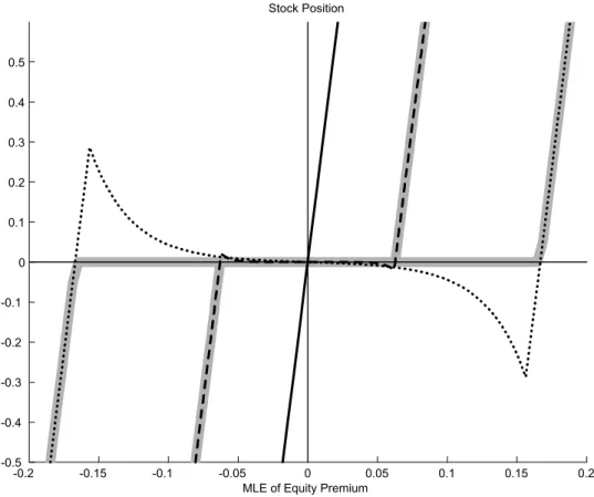
Optimal portfolios
Learning under ambiguity affects portfolio choice in two ways. The first is a direct effect of beliefs and confidence on the optimal weight which is relevant at any investment horizon. In particular, the optimal stock weight of a myopic investor (T = 1/k) is, fork