Spectrum Access Systems
A thesis submitted in fulfilment of the requirements for the degree of
Doctor of Philosophy
Hamid Eltom
B.Sc (Honours) Electrical and Electronics
University of Khartoum
School of Engineering
College of Science, Engineering and Health
RMIT University
I declare that this thesis does not incorporate without acknowledgement any material previously submitted for a degree or diploma in any university, and that to the best of my knowledge it does not contain any materials previously published or written by another person except where due reference is made in the text.
I acknowledge the support I have received for my research through the provision of an Australian Government Research Training Program Scholarship.
This research was supported under Australian Research Council’s Discovery Projects funding scheme (Cognitive Radars for Auto-mobiles, DP150104473).
Hamid Eltom February 2018
For: Najat Hamid
To: Najat Hamid
I would first like to thank my thesis advisor A/Professor Kandeepan Sithampara-nathan. The door to Prof. Sithamparanathan office was always open whenever I ran into a trouble spot or had a question about my research or writing. He/She consistently allowed this paper to be my own work, but steered me in the right the direction whenever he thought I needed it. I would like to thank my fellow doctoral students for their feedback, cooperation and of course friendship.
I would like to thank my friends for accepting nothing less than excellence from me. Last but not the least, I would like to thank my family (My wife Amira, my sister Salma, and my father) for supporting me spiritually throughout writing this thesis and my life in general.
This research was supported under Australian Research Council’s Discovery Projects funding scheme (Cognitive Radars for Auto-mobiles, DP150104473)
List of tables vi
List of figures vii
Abstract 1
1 Introduction 3
1.1 Background . . . 3
1.2 Motivation . . . 5
1.3 Spectrum Occupancy Prediction Overview . . . 5
1.3.1 Spectrum Occupancy Classification . . . 6
1.3.2 Statistical Prediction . . . 8
1.3.3 Bayesian Based Spectrum Prediction . . . 8
1.3.4 Cooperative spectral prediction . . . 9
1.4 Mathematical Preliminaries for Spectrum Occupancy Prediction . . . . 9
1.4.1 Some Theoretical Preliminaries . . . 10
1.4.2 Spectrum Sensing in Dynamic Spectrum Access . . . 12
1.4.3 Hidden Markov Model . . . 14
1.4.4 Mean Prediction Error . . . 17
1.5 Research Questions and Contribution . . . 19
1.5.1 Contribution Summary . . . 21
1.5.2 Publications . . . 23
1.6 Thesis Structure . . . 23
2 Prediction Model Classification 25 2.1 Background . . . 26
2.2 Statistical Prediction . . . 28
2.2.2 Deterministic Settings . . . 29
2.2.3 Loss Function and Regret . . . 29
2.2.4 Bayesian Methods for Source Assignment . . . 30
2.3 Empirical Spectrum Occupancy Prediction . . . 32
2.3.1 Spectrum Measurement campaigns . . . 33
2.3.2 Statistical occupancy modelling . . . 34
2.4 Memoryless Stochastic Source Models . . . 41
2.5 Finite order Markov Models . . . 42
2.6 Finite Order Linear Regression Models . . . 45
2.7 Machine Learning based Techniques . . . 46
2.8 Extending Occupancy Prediction Formulation . . . 47
2.9 Spectrum Occupancy Prediction Challenges . . . 47
2.9.1 Validity and Complexity . . . 48
2.9.2 Cooperation and Contention . . . 49
2.10 Summary . . . 49
3 Local Spectrum Occupancy Prediction 50 3.1 Background and Related Work . . . 51
3.1.1 HMM for spectrum occupancy modelling . . . 51
3.1.2 HMM posterior probability estimation . . . 52
3.2 Local SOP Model Formulation . . . 53
3.2.1 Primary User Activity Model . . . 53
3.2.2 Channel Propagation Model . . . 54
3.2.3 Occupancy Detection Model . . . 55
3.2.4 Local Spectrum Prediction Model . . . 56
3.3 Theoretical Analysis . . . 58
3.3.1 Ideal Sensing (Markov chain) . . . 59
3.3.2 Non-ideal Sensing (HMM) . . . 61
3.3.3 Generalized Beta-Bernoulli approximation of local prediction error 62 3.4 Case Study Analysis . . . 64
3.5 Summary . . . 70
4 Cooperative Spectrum Prediction based on Hard Fusion 71 4.1 Background and Related Work . . . 72
4.2 Cooperative Prediction Model Formulation . . . 73
4.3.1 Cooperative Prediction Error . . . 75
4.3.2 Binomial approximation for cooperative SOP Error . . . 76
4.3.3 Generalized Beta-Binomial approximation of cooperative Pre-diction Error . . . 77
4.4 Case study analysis . . . 80
4.5 Summary . . . 86
5 Cooperative Soft Fusion for HMM based Spectrum Occupancy Pre-diction 87 5.1 Introduction . . . 88
5.2 System Model . . . 89
5.2.1 Primary user activity model . . . 89
5.2.2 Occupancy Observation Model with Spectrum Sensing . . . 90
5.2.3 Local spectrum prediction model . . . 91
5.3 Soft cooperative Prediction Techniques for Spectrum Occupancy . . . . 92
5.3.1 Maximal-Ratio Based Soft Fusion . . . 92
5.3.2 Equal-Gain Based Soft Fusion . . . 94
5.3.3 Selection Combining Based Soft Fusion . . . 94
5.4 Performance analysis . . . 94
5.5 Summary . . . 99
6 Conclusion and Future Work 100
1 Notations and Symbols . . . x
2.1 Summary of spectrum prediction technique . . . 39
2.2 Comparison of Spectrum prediction categories . . . 40
3.1 Local Prediction simulation parameters . . . 64
5.1 Simulation Parameters . . . 95
1.1 An example of spectrum sensing and access in a typical DSA
time-slotted system. . . 4
1.2 Spectrum prediction in dynamic spectrum access framework . . . 7
1.3 Spectrum occupancy prediction flowchart . . . 10
1.4 HMM Prediction Flow chart . . . 17
2.1 Spectrum occupancy prediction flowchart (this figure is repeated for the convenience of the reader) . . . 33
2.2 Power measurement campaign sample for Melbourne LTE system mea-surements [1] . . . 34
2.3 Sequential prediction classification of spectrum prediction techniques . 36 2.4 Statistical prediction using Markov based models . . . 45
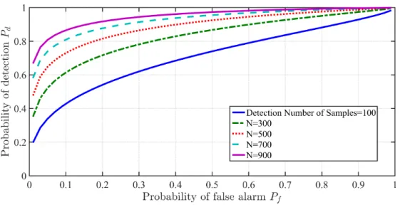
3.1 Energy Detector ROC Curve for different values of ρr (N = 1000) . . . 55
3.2 Energy Detector ROC Curve for different values ofN ( SNR ρr dB = -10) . . . 56
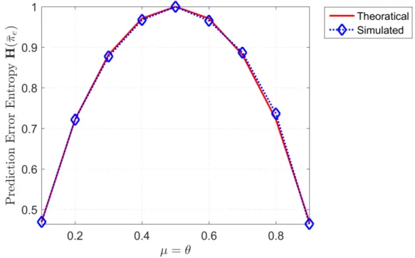
3.3 Prediction Error Entropy . . . 60
3.4 Beta Bernoulli Approximation of HMM prediction error . . . 63
3.5 Prediction Error as a function of observation sequence length . . . 66
3.6 Single User prediction Error Vs. Channel occupancy probability. . . 66
3.7 Prediction Error Vs probability to remain in specific state, Equal Sta-tionary Distribution case . . . 67
3.8 Single User prediction Error Vs. Channel Errors . . . 68
3.9 Prediction Detection ¯πd vs Channel Errors (Pm for different Pf values) 68 3.10 Prediction False alarm ¯πf vs Channel Errors (Pm for different Pf values) 69 3.11 Prediction Error for second Slot (Given error in the first prediction) VS miss-detection probability . . . 69
3.12 Prediction Error for second Slot (Given error in the first prediction) VS
probability to remain in busy state . . . 70
4.1 Cooperative Hard Fusion Spectrum Occupancy Prediction . . . 74
4.2 GBB Hyper-parameters . . . 78
4.3 GBB approximation of hard fusion mean prediction error . . . 79
4.4 Mean prediction error Vs number of users (15 Users) . . . 80
4.5 Mean Prediction Error forµ=θ (15 users) . . . 80
4.6 Cooperative Prediction Error for Hard Combining, for 3/5/15 Users, for Majority Rule . . . 81
4.7 Cooperative Prediction Error, Hard Combining for 3/5/15 Users for OR/AND Rules . . . 82
4.8 Cooperative prediction miss-detection Error, Hard Combining for 3/5/15 Users for Majority Rule . . . 83
4.9 Cooperative prediction false alarm Error, Hard Combining for 3/5/15 Users for Majority Rule . . . 83
4.10 Prediction false alarm Error, Hard Combining for 15 Users for Pm =Pf 84 4.11 Prediction miss detection Error, Hard Combining for 15 Users forPm =Pf 84 4.12 Prediction miss detection Error, Hard Combining for 15 Users . . . 85
4.13 Prediction false alarm Error, Hard Combining for 15 Users . . . 85
5.1 Local and Cooperative Spectrum Prediction Model . . . 90
5.2 Comparing the soft fusion mean prediction error for 15 SUs . . . 96
5.3 Comparing the soft fusion mean prediction error for different number of SUs . . . 97
5.4 Soft fusion mean prediction error under different shadowing levels . . . 97
5.5 soft fusion mean prediction error for different probability of false alarm values . . . 98
CR Congitive radio
CFAR Constant false alarm DSA dynamic spectrum access ED Energy detector
EG equal gain HF hard fusion
HMM hidden markov mode IoT intrent of things
MRC maximum ratio combining PU primary user
SOP spectrum occupancy prediction SC selection combining
SU secondary user SF soft fusion
WRAN Wireless Regional Access Networks SNR signal to noise ratio
Table 1 Notations and Symbols
X Vector or matrix
E[·] Expectation operator
V[·] Variance operator
det(·) Determinant of a matrix
I Identity matrix
1 Column vector of ones
[·]T Transpose operator
Despite the remarkable foreseen advancements in maximizing network capacities, the in-expansible nature of radio spectrum exposed outdated spectrum management tech-niques as a core limitation. Fixed spectrum allocation inefficiency has generated a proliferation of dynamic spectrum access solutions to accommodate the growing de-mand for wireless, and mobile applications.
This research primarily focuses on spectrum occupancy prediction which equip dy-namic users with the cognitive ability to identify and exploit instantaneous availabil-ity of spectrum opportunities. The first part of this research is devoted to identifying candidate occupancy prediction techniques suitable for SOP scenarios are extensively analysed, and a theoretical based model selection framework is consolidated. The performance of single user Bayesian/Markov based techniques both analytically and numerically. Understanding performance bounds of Bayesian/Markov prediction al-lows the development of efficient occupancy prediction models. The third and fourth parts of this research investigates cooperative decision and data-based occupancy pre-diction. The expected cooperative prediction accuracy gain is addressed based on the single user prediction model. Specifically, the third contributions provide analyt-ical approximations of single user, as well as cooperative hard fusion based spectrum prediction. Finally, the forth contribution shows soft fusion is superior and more ro-bust compared to hard fusion cooperative prediction in terms of prediction accuracy. Throughout this research, case study analysis is provided to evaluate the performance of the proposed approaches. Analytical approaches and Monte-Carlo simulation are compared for the performance metric of interest. Remarkably, the case study analysis confirmed that the statistical approximation can predict the performance of local and hard fusion cooperative prediction accurately, capturing all the essential aspects of signal detection performance, temporal dependency of spectrum occupancy as well as the finite nature of the network.
• H. Eltom, S. Kandeepan, B. Moran, and R. J. Evans, “Spectrum occupancy
prediction using a hidden Markov model” 2015 9th International Conference on Signal Processing and Communication Systems (ICSPCS), Dec 2015 [2].
• H. Eltom, S. Kandeepan, Y. C. Liang, B. Moran, and R. J. Evans, “HMM
based cooperative spectrum occupancy prediction using hard fusion,” 2016 IEEE International Conference on Communications Workshops (ICC), May 2016 [3]. • H. Eltom, S. Kandeepan, R. J. Evans, Y. C. Liang, and B. Ristic,"Statistical
Spectrum Occupancy Prediction for Dynamic Spectrum Access: A Classification ", EURASIP Journal on Wireless Communications and Networking, February 2018 [4].
• Hamid Eltom, Sithamparanathan Kandeepan, Y.C. Liang, and Robin J.
Evans,"Cooperative Soft Fusion for HMM based Spectrum Occupancy Predic-tion", Submitted to IEEE Communications letters.
• Hamid Eltom, Sithamparanathan Kandeepan, Y.C. Liang, and Robin J.
Evans,"An approximation of stationary posterior distribution of HMM based Spectrum Occupancy Prediction", Submitted to IEEE Communications letters. • Hourani, A., Evans, R., Sithamparanathan, K., Moran, W., Eltom, H. "
Stochastic Geometry Methods for Modelling Automotive Radar Interference In: IEEE Transactions on Intelligent Transportation Systems, 2017 [5] .
Introduction
1.1
Background
The ubiquity of mobile phones and Wi-Fi access points overemphasises the impending age of Internet of things (IoT), which intuitively projects an exponential increase in demand for wireless data traffic. The seemingly augmenting mobile services sub-scription rate as well as the proliferation of mobile media consumption overshadows the efforts by the wireless communication industry to fulfil the requirements for next generation communication systems. The anticipated (1000x) demand factor in data traffic, which was set as a target requirement for (5G) networks, manifests the axiom of exponential increase in wireless data traffic. Advanced receiver design, multi-antenna techniques accompanied by cooperative and heterogeneous networks deployments, actualized the current innovative state of wireless communication development to address the increasing demand. However, despite the remarkable foreseen advancements in maximizing network capacities, the in-expansible nature of radio spectrum exposed outdated spectrum management techniques as a core limitation. Spectrum scarcity is the paradigm that describes the artificial problem in spectrum sharing regulation policies created by inefficient allocation of frequency bands [1,6, 7].
Fixed spectrum allocation inefficiency has generated a proliferation of dynamic spectrum access solutions to accommodate the growing demand for wireless, and mo-bile applications. Software-defined radios (or cognitive radio) networks which offer a dynamic spectrum access management policy of fixed allocated licensed bands, could potentially solve the artificial spectrum scarcity problem. Dynamic Spectrum Access
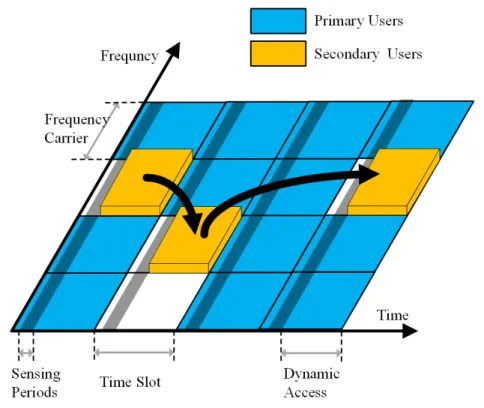
Fig. 1.1 An example of spectrum sensing and access in a typical DSA time-slotted system.
(DSA) systems typically consist of licensedPrimary users (PU’s), and opportunistic
Secondary users (SU’s). Primary users are the incumbent owners of the spectrum,
while the secondary users opportunistically access the spectrum, and are required to inflict limited interference on the primary users (Fig.1.1). To fulfil such requirements, secondary users must be equipped with a cognitive ability, and reconfigurability, to identify and exploit instantaneous availability of spectrum opportunities (holes) [6,8]. Spectrum management framework classifies such cognitive ability into few generic func-tions, referred to as cognitive radio cycle functions. These functions are represented by the secondary user’s ability to preform spectrum Sensing, Decision, Sharing, and Mobility [8,9]. Spectrum occupancy prediction (SOP) models were proposed in DSA
literature to optimize cognitive cycle functional processing time [10]. SOP models add agility, and adaptability to cognitive radio functions to optimize processes such as periodic spectrum sensing scheduling, and channel selection in spectrum decision [8]. Similarly, SOP models allow the implementation of a proactive spectrum mobility strategy based on predicted occupancy patterns which avoids collisions with incumbent primary users [10, 11]. The resource efficiency that spectrum prediction potentially
adds to dynamic spectrum access, emphasizes the importance of this cognitive radio enabling process.
1.2
Motivation
Despite the crucial role of spectrum prediction in enabling cognitive radio to efficiently utilize spectrum opportunities, spectrum prediction literature is scarce. Current literature on spectrum prediction in DSA systems lacks a consolidated framework for model selection, as well as prediction performance analysis. Additionally, candidate prediction techniques suitable for SOP scenarios are not extensively classified nor immediately identified. Current framework of prediction model selection is application dependent where SOP proposals restrict the model validity to a specific technology scenario. While several proposals simulated Bayesian/Markov based prediction models for different wireless technologies, the abstract ability of these models to provide accurate occupancy modelling and prediction is still not intuitively clear [10]. In other words, the functional relationship between prediction performance measures and model parameters are not explicitly studied, formulated nor approximated.
In this thesis, performance analysis of spectrum prediction is the primary focus. In particular, this research is devoted to explore the performance of Bayesian/Markov based techniques (namely, Hidden Markov Model HMM) both analytically and
nu-merically. Understanding performance bounds of HMM based prediction allows the development of efficient SOP models. An extensive review of sequential prediction in cognitive radio is pursued to identify the statistical framework of prediction model se-lection. Then, numerical recursive techniques and statistical approximations of single, and multi-user spectrum prediction performance analysis are proposed. Section-1.3
provides an overview of spectrum occupancy, while Subsection-1.4 provides an intro-duction into the proposed HMM model.
1.3
Spectrum Occupancy Prediction Overview
The motivation for SOP models is to minimize the accumulatedtime delaydue to cog-nitive cycle serial functional processing. By predicting the channel status in advance, more processing time becomes available for spectrum sensing, decisions, and mobility (Fig.1.2) [10]. Performance gains of SOP can is manifested in the context of:
• Wireless Regional Access Networks WRAN (802.22); TV UHF/VHF bands
attracted attention as an ideal candidate to provide high speed data com-munication, due to its appealing radio characteristics (low noise, reasonable antenna size and line of sight). As analogue TV bands are being unused with the dominance of digital TV; these UHF/VHF bands represent an opportunity to provide valuable growth capital for service providers [12]. 802.22 WRAN
provides two methods of obtaining spectrum occupancy, 1) through geo-location and database, and 2) through spectrum sensing. Spectrum occupancy predic-tion is a potentially valuable asset in optimizing 802.22 sensing and dynamic spectrum access abilities. Through additional layer of machine learning, cognitive radio networks are able to opportunistically utilize the spatial/ tem-poral spectrum opportunities to provide data access in WRAN white TV spaces. • Consumer Cognitive Radar (DSA cognitive radar) [7, 13–15]: Cognitive radar is a concept developed by S. Haykin as the future of fully adaptive and efficient radar that adjusts its parameters for faster and more accurate surveillance [14]. Though dynamic spectrum access was not initially proposed since the intended application was predominantly military focused; consumer radar adopting both DSA and cognitive radar concepts is a new realization of the cognitive radar[15]. Consumer radar with DSA capabilities can be realized in vehicular and/or aerial scenarios. Such radar would make an efficient use of limited shared spectrum bands, while providing intelligent collision avoidance and environment awareness. One feasible scenario involves collision avoidance for vehicle highway scenario [1]. The motivation in this thesis to address this particular application stems from the ARC project for automotive radar interference mitigation/avoidance [5] (76-77 GHZ band set by the Australian Communication Authority for automotive radars [16]).
1.3.1
Spectrum Occupancy Classification
Unless specified otherwise , in the cognitive DSA system design such as 802.22 [12], spectrum occupancy state is the result of the stochastic sampling process of radio environment. However, typical stochastic sampling intuitively carries stochastic randomness gained from combination of sampling process accuracy and/or underly-ing stochastic activity patterns [17]. Spectrum occupancy prediction models target
Fig. 1.2 Spectrum prediction in dynamic spectrum access framework
the usage of spectrum bands utilized by both incumbent users, and opportunistic users. SOP models broadly target parameters such as channel availability i.e. pre-diction of channel status as idle or busy, as well as duty cycle i.e. prediction of the average fraction of time the primary user is occupying the channel [1, 18]. In the DSA literature, spectrum occupancy prediction techniques address prediction ei-ther explicitly [19–21], or implicitly. Implicit approaches present SOP models as pri-mary/secondary user’s occupancy/activity models. Statistical SOP models proposed for spectrum occupancy analysis include Poisson processes [22, 23], Bayesian predic-tion [24, 25], and linear regression [26, 27]. Machine learning based techniques have also been proposed for modellearning including neural networks, time regression, and space vector machines [10, 28, 29]. The framework of current research into spectrum occupancy can be divided into the following generic categories:
• Measurement campaign modelling: An empirical research conducted in specific scenarios (indoor, outdoor) to collect real life data using an antenna that covers specific frequency band. Statistical analysis, averaging and maximization are conducted to generate an approximate statically density functions and/ or simple statistical description of power, channel occupancy, etc. Though such modelling
is able to capture the real life data, it is however, riddled with inaccuracy, spatial and temporal dependency[18].
• Statistical primary user modelling and prediction: Statistical modelling aims to find the best suitable stochastic procedure that describes a specific primary user(s) mode of operation and its channel utilization. Given such statistical esti-mation, prediction of possible presence of absence in future instances is possible [10,11].
Chapter-2 elaborates on spectrum prediction classification and presents our pub-lished framework and review on spectrum prediction in dynamic spectrum access sys-tems. The basis of the proposed framework is the sequential statistical prediction introduced in next the section as well as Chapter-2.
1.3.2
Statistical Prediction
Statistical prediction in it’s simplest form is: "Given an observation sequencex1:t−1 up
to time instant t−1, and before the symbol at timetis revealed the predictor guesses
the next value xt based on the previous t−1 observations ". The observations are
assumed to follow a stationary stochastic process, and thus statistical properties can be derived from the past observations and an effective rule can be postulated from these statistics. The predictor measures the loss function between the actual value and the predicted value. The loss function measures the quality of the prediction and provides the input to compare prediction rules [17,30]. Based on the main components of the statistical prediction problem presented in Chapter-2, HMM (in the next subsection) is introduced in Section-1.4, and more details are presented in Chapter-3.
1.3.3
Bayesian Based Spectrum Prediction
Bayesian-based prediction techniques provide powerful, and flexible tools to learn and adapt to the radio environment. Secondary users within the cognitive radio network, collect sensing information, and utilize statistical correlation, to infer possible future states of the primary user usage patterns. Bayesian Mixture models scenario are extensively studied in information and coding theory [31–33]. Bayesian algorithms are minimax optimal, and are universal under self information loss functions [34–
36]. The algorithms perform well under both probabilistic and deterministic non-stochastic settings [31, 34, 35, 37, 38]. Additionally, Markov-based construction is
attractive due to the desirable convergence properties of Markov chain based models [39–42]. Markov chain, andpartially observable Markov models are commonly used for spectrum occupancy modelling. Chapter-3 considers single user prediction scenarios are based on HMM system model.
1.3.4
Cooperative spectral prediction
Spectrum prediction in single secondary user environment is commonly known as local spectrum prediction. Consequently, cooperative spectrum prediction in multi-user environment was proposed to improve the collective accuracy of spectrum occupancy prediction [43, 44]. Cooperative fusion of secondary user’s decisions has been studied extensively in DSA based solutions to address diverse optimization problems. A multitude of decision fusion techniques were used such as hard and soft for temporal and, spatial fusion for local node decisions [45]. Combined decision fusion and Bayesian estimation has been also suggested for decentralized tracking [46]. In spectrum occupancy prediction literature, cooperative spectrum prediction fu-sion was only studied in handful of papers such as [20] where a coalition based game theory approach was implanted for a multi-primary/secondary users environment. The study showed general improvements when using cooperative prediction, but the results lacked fine details of improvement in terms of dependency on traffic load, and/or de-tection accuracy. Chapter-4and Chapter-5 focus on hard and soft fusion of spectrum prediction decisions, respectively.
1.4
Mathematical Preliminaries for Spectrum
Oc-cupancy Prediction
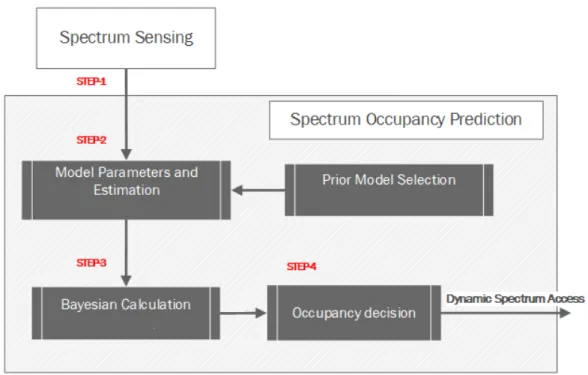
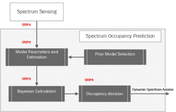
The flow chart in Fig-1.3 highlights the sequence of spectrum occupancy prediction process. Spectrum sensing provides occupancy observations for local spectrum pre-diction. Given the selected prediction model (Chapter-2), the model parameters are estimated based on a training sequence. Then, Bayesian methods are used to esti-mate the probability that the next spectrum opportunity is available. Finally, using a predefined threshold the prediction decision is made and passed to spectrum de-cision function. This section provides background information on spectrum sensing, hidden Markov models, and maximum likelihood estimation Baum Welch algorithm
[47]. Background and related contents contained in this section are used for system models in Chapter-2, and statistical analysis of spectrum prediction in Chapter-3and Chapter-5.
Fig. 1.3 Spectrum occupancy prediction flowchart
1.4.1
Some Theoretical Preliminaries
The theories and mathematical background in this subsection are the basis of statis-tical analysis for SOP models in Chapter-3 and Chapter-5, as well as Section-1.4.3.
To estimate the probability of error in estimation of a random variable, Fano inequality serves as bound for error probability, and definitions of Markov chain sta-tionary distribution, Cesáro mean, and Entropy rate are needed to derive such ap-proximation.
Theorem 1.4.1 (Cesáro Mean). Cesaro mean for convergent sequences states
regarding the arithmetic mean states [48]: let an → A, let bn = n1 n P i=1 ai, then lim n→∞bn =A.
Theorem 1.4.2 (Entropy Rate). Entropy rate of a stochastic processXn is defined
by H(X) = lim
n→∞
1
nH(X
the other notion of entropy rate defined as H′(X) = lim
n→∞H(Xn|X
n−1).
Theorem 1.4.3 (Fano Inequality). letXbe a random variable with finite outcomes in X, let Xˆ =g(Y) be an estimated value of X for some deterministic function of g that takes values in X, then the loose probability of error bound is stated as [38]
pe △ =pe(Xˆ ̸=X)≥ H(X|Y)−1 log|X | or more strongly as H(Ber(pe)) +pelog(|X −1|)≥H(X|Y)
Where H(X|Y) =Ep(x,y)log2 1
p(x|y), and Ber(pe) is error Bernoulli random variable.
Distance measure Following [31], instantaneous Distance, and total distance be-tween probability distributions P, Qw are defined as:
dt(xt|x0:t−1) := X xt−1 P(xt|x0:t−1) ln P(xt|x0:t−1) Qw(xt|x0:t−1) , Dn:= n X t=1 E[dt].
Where dt is the instantaneous KL divergence. While Dn is the total distance
counterpart. Dn is chosen as the distance measure in Section-1.4.
Beta-Bernoulli Distribution Bernoulli random variable X takes only the values
0 or 1 representing failure and success, respectively. The probability mass function parametrised by ρ the probability of success is:
ρ =p(X = 1)
f(k;ρ) =ρk(1−ρ)(1−k), k∈ {0,1}
Ifρ is assumed to be drawn from a random distribution, then the conjugate prior
distribution is then a Beta distribution given by:
p(ρ|α, β)∼Beta(α, β) α, β >0 p(ρ|α, β, a, b) = (ρ) α−1(1ρ)β−1 B(α, β) B(α, β) = Z 1 0 tα−1(1−t)β−1dt
whereB(α, β) is the standard beta function. The posterior predictive distribution
is the compound distribution given by :
f(k|α, β) = B(k+α,1−k+β)
B(α, β)
The Beta-Bernoulli distribution is a special case of the Beta-Binomial distribution [49,50] for the number of successes k inn trials :
f(k|n, α, β) = Γ(n+ 1)
Γ(k+ 1)Γ(n−k−1)
B(k+α, n−k+β) B(α, β)
Beta-Bernouli and Beta-binomial are used in Chapter-3/Chapter-4 for the pro-posed approximation of local, and cooperative prediction error distribution, respec-tively.
1.4.2
Spectrum Sensing in Dynamic Spectrum Access
Spectrum sensing provides a method of using the spectrum more efficiently. Spectrum sensing enables cognitive radio devices to access, and monitor free sections of radio spectrum. Cognitive radio must relay on spectrum sensing to keep monitoring the spectrum to avoid undue interference. Sensing functions must then be able to detect other transmissions, and identify the sources.
Cognitive Radio Spectrum Sensing Basics
Spectrum sensing provides the instantaneous occupancy status of every spectrum opportunity. Consequently, spectrum sensing algorithms must accommodate several considerations to effectively coexist in a multi-user environment. Sensing must be continuous to avoid causing interference to primary users, but also to identify alter-native spectrum availabilities. Sensing cognitive ability to recognize the transmission source and type in order to identify spurious interference sources is crucial element of the functionality.
Spectrum sensing can be also performed in a cooperative manner where several radio units to improve sensing robustness to hidden sources. However, parameters such as sensing bandwidth and transmission type identification are the some of the key challenges to sensing algorithm design. Additionally, accuracy and window timing
control the efficiency of spectrum sensing utilization of available spectrum opportuni-ties. Signal detection techniques used in spectrum sensing includes energy detectors, cyclostationary, matched filter and Bayesian detectors. Basic energy detector is de-scribed in subsection-1.4.2 along with correct/incorrect detection probabilities. Each secondary user prediction performance relies on spectrum sensing accuracy. The re-sults in Chapter-3and Chapter-5are presented against sensing detection probabilities, as well as HMM model parameters (subsection-1.4.3) [45].
Spectrum Detection Accuracy
The received signal zr,t is detected by a complex baseband equivalent of an energy
detector. The two hypothesis of present, and absent signals for an observation period of T or the equivalent ofN samples for each time slot t. Test statistics Φz,r,t for time
slot tfor a large number of samplesN is assumed to be Gaussian distributed (Central
limit Theorem) [51]. The test statistic of the analogue energy detector can be given as: Φz,r,t ∼ N( N X i=1 E[|zir,t|2], N X i=1 V[|zr,ti |2]) (1.1) E[|zir,t|2] =σ2 wr +θ|s i t| 2 V[|zr,ti |2]) = (σ2 wr) 2+θσ2 w|s i t|2 (1.2)
wherest is the transmitted signal, channel noise is assumed as a zero mean
Gaus-sian noise wr with variance σ2wr, and θ = [0,1] the null and alternative hypothesis, respectively. ρr = 1 N PN i=1|sit|2 σ2 wr (1.3) Hypothesis testing on the detection statistics yields the the series yr,t i.e., the
oc-cupancy perceived by each SU. The uncertainty around spectrum sensing performance is quantified by the probability of correct detection Pd(r), and the probability of false
alarm, and Pf(r) can be defined using central limit theorem approximation for large
Pf(r)≈Q( λ−N σ2 w √ N σ2 w ) (1.4) Pd(r)≈Q( λ−√N σ2 w(1 +ρr) √ N σ2 w(1 +ρr) )
The probability of detectionPd= 1−Pmis the probability of successfully observing
the channel correctly as busy where Pm is the miss-detection probability, and the
probability of false alarm Pf is the probability of observing occupied channel while
the primary user is idle. For constant false alarm based approaches (CFAR), the
threshold λin is calculated, for a large number of samplesN using inverse Q-function
1.4.3
Hidden Markov Model
This section describes the estimation and training of hidden models analysed in Chapter-3. HMM is the proposed system model for single/multi user spectrum predic-tion occupancy as seen by the secondary user, which is used in in Chapter-3, Chapter-4, and Chapter-5. Markov-based construction is attractive due to the desirable conver-gence properties of Markov chain based models [39–42]. Markov property describes the case when the probability of current event xt only depends on the probability of
previous event xt−1 i.e., p(xt|xt−1) = p(xt|xt−1) [48]. The Discrete-Time HMM can be
fully defined as follows:
λ = (△ P,E,v) (1.5) v =△ p(x0 =i), :i∈ {1, ..K}. P=△ p(xt=j|xt−1 =i) :j ∈ {1, ..K}. Er △ =p(yr,t =k|xt=j) :k ∈ {1, ..L}.
Where Pis the hidden state transition matrix, Lis the total number of hidden states, Er is the observation emission matrix, K is the total number of possible observation
states, and v is the initial state vector.
Event Space and transition matrix
The two state of a primary user activity in a frequency channel are Idle and Busy. Define {xt : t ≥ 1}, x ∈ {0,1} as the channel state at time slot t as irreducible
stationary Markov chain. The transition probability matrix between states i, j ∈[0,1] i.e. p(xt=j|x0, .., xt−1 =i) =p(xt|xt−1 =iis given by [48]: P= [pij] = p1,1 p1,2 p2,1 p2,2 (1.6)
Where P is a transition probability matrix for all time instants 1..t. Observation Space, and the emission matrix
In a two state hidden Markov model, observations are independent and identically distributed random variables. The two hypothesis of a secondary user’s perceived occupancy are present, and absent. The relation between the observation sequence
y1:t, and the hidden event space is the emission matrix that represents the probability
of an observation is an outcome of a specific hidden state. The emission matrix is designed as follows : E = [eij] = e1,1 e1,2 e2,1 e2,2 (1.7)
Secondary user’s model is a hidden Markov model characterized by the transition
P, and emission Er matrices, as well as the initial state distribution p(x0). The
observation sequenceyr,t is characterised by the emission matrixEr of each SU which
maps Markov chain based PU channel activity x1:t to the perceived SU spectrum
occupancy y1:t: Er = 1−Pf(r) Pf(r) 1−Pd(r) Pd(r) r∈ {1,2, .., R} (1.8)
HMM Estimation and Forward-Backward algorithm
For a finite state space HMM, local prediction utilizes forward backward algorithm to estimate the joint posterior probability of primary user activity and secondary user’s observation sequences p(ˆx0:t, y1:t−1) [52]. Define ˆxt, x ∈ [0,1] as the predicted state
value by SU: p(ˆx0:t, y1:t−1) = p(x0) " t Y n=1 p(xn|xn−1) #t−1 Y n=1 p(yn|xn) (1.9)
as the probability of the next state given a vector of past observations. Using the Bayesian definition of joint posterior probability relation:
p(ˆxt|y1:t−1) =
X
ˆ
xt=i
p(xt|xt−1)p(xt|y1:t−1) : i∈ {1,2}. (1.10)
The last term in the equation above, represents the predictive posterior probability at time instant t given the observation sequence. This posterior probability can be calculated using the Forward-Backward algorithm. The forward probability αt(i) = p(y1:t−1, xt=i) is calculated recursively for a observation vector y1:t:
αt−1(i) =p(y1:t−1, xt−1 =i), 1≤t≤T −1 (1.11) α1(i) =p(x0 =i)p(yt|xt=i) :i, j ∈ {1,2} αt(j) =p(yt|xt=j) " 2 X i=1 αt−1(i)p(xt=j|xt−1 =i) # (1.12) p(y1:t) = 2 X i=1 αT(i) (1.13)
While the backward probabilityβt(i) =p(yt+1:t, xt=i) the probability of observing
all future events from this state. Since the initial state is assumed as given (i.e. the prior probability of this state = 1). The backward probability is calculated recursively for a observation vector yt+1:1:
βt(i) =p(yr,t+1:T, xt=i), t=T −1, T −2, ...,1 (1.14) βT(i) = 1 βt(j) = 2 X i=1 βt+1(j)p(xt=j|xt−1 =i)p(yt+1|xt=j) (1.15)
The Forward-Backward algorithm computes the expectation of how often each transition/emission is used, and repeats until convergence.
Staring with initial estimates of the transition and emission matrices, Baum-Welch training iteratively recalculates each matrix probabilities from the training sequence using (Equations-1.14and Equation-1.11), then uses the outcome to estimate the state transition matrices. Baum-Welch algorithm is special case of the Expectation Maximization (EM) algorithm. HMM posterior probability is non-stationary random
variable, and is a function of the observation series. Thus, analytical expression of the stationary conditional predictive posteriori (and hence error probability in
Subsection-1.4.4) is counter-intuitive, and hard to obtain in a closed form for arbitrary HMM
models [35, 53]. In Summary, HMM prediction follows the general steps (Fig.1.4): • HMM Training: the observation sequence is used to train the HMM, and
re-estimate the model parameters. The transition, and the emission probabilities are calculated using Baum-Welch algorithm.
• HMM decoding: to estimate the hidden state corresponding to the observed sequence. Forward algorithm is used to calculate the corresponding posterior probability of the hidden state given the observed sequence.
• HMM prediction decision is hypothesis testing of the SU predicted value ˆxt
• Instantaneous error function calculation of the SU predicted occupancy value ˆxt
against the actual system state xt (Subsection-1.4.4).
Channel Occupancy Sequence HMM Training λ Posterior Probability Estimation Next State
Probability Binary Hypothesis
Testing Access decision
Next Slot Prediction
Fig. 1.4 HMM Prediction Flow chart
1.4.4
Mean Prediction Error
Under the two state ON/OFF model, prediction error is a Bernoulli random variable (Et, where Et= ˆxt⊕xt, Et ∈ {0,1}). πt the error in prediction at time instant t, and
πt = P(Et= 1) ¯ πe = lim t→∞E(πt) = limn→∞ 1 n n X i=1 (πi) (1.16)
The existence and equality in (1.16) requires the convergence of the quantity
p(ˆxt|y1:t−1) according to Cesáro Mean (Theorem-1.4.1). Additionally, define the local
(prediction) miss-detection ¯πd, and false alarm probability ¯πf as:
¯
πf = ¯πep(xt= 0)
¯
πd= (1−π¯e)p(xt= 1)
to indicate mean prediction error for busy and idle channels, respectively. Ad-ditionally, the conditional entropy rate of prediction probability (Theorem-1.4.2) is given by: H(ˆxt|y1:t−1) = limt→∞Ep(ˆxt,y1:t−1)log2 1 p(ˆxt|y1:t−1) (1.17) H(ˆxt|y1:t−1) = limt→∞H(ˆxt|y1:t−1) (1.18)
UsingFano Inequality(Theorem-1.4.3), the mean prediction error ¯piecan be loosely
bounded [38]:
¯
πe ≥
H(ˆxt|y1:t−1)−1
log(|R|) (1.19)
Where p(ˆxt|y1:t−1), or using the tighter Fano bound (Theorem-1.4.3):
H(¯πe)≥ H(ˆxt|y1:t−1)
The entropy rate for finite Markov processes is studied by Blackwell in [40] using a probability distribution on a Borel set of measures expressed using a integral that is hard to evaluate. A closed form expression for (1.16) requires the calculation of the limiting distribution of p(ˆxt|y1:t−1). Such expression requires the calculation of
convergence of non-stationary Markov chain. Thus, mean prediction error required the complete characterisation of the predictive posterior probability (p(ˆxt|y1:t−1)).
1.5
Research Questions and Contribution
Based on the literature review conducted in this work as presented in Chapter-2, three research questions were formulated. In general the literature review presented can be summarized into the following:
• Existing methods for statistical prediction. • Existing work on spectral occupancy modelling.
• Existing limited work on spectrum occupancy prediction.
Based on the literature review the gaps in the research conduced so far and the scope for improving the techniques were identify, which are formulated as research questions as given below:
Research Question 1: How accurate is Bayesian spectrum
pre-diction with information uncertainty and error? What are the
mean prediction error characteristics?
Under this research question, spectrum prediction under the family of Bayesian models is investigated. The performance of a secondary user prediction is studied against the error introduced by wireless channel, and sensing/sampling process. These errors can be quantified as detection error, and false alarm probability. The relation is studied for different scenarios of primary user activity patterns as well as channel conditions. Monte-Carlo simulations are utilized to investigate mean prediction error for HMM based spectrum prediction models. Then, a practical approximation of mean prediction error is constructed as a function of HMM model parameters. The expected deliverables outcome of this research question will include:
• A practical and tractable model selection framework based on sequential predic-tion theory.
• Numerical performance analysis of single user HMM based spectrum prediction. • Numerical approximation of HMM prediction error as a function of model
Research Question 2: How can multi-user cooperation improve
the spectral prediction performance? How well Hard fusion
based prediction fares compared to local spectrum prediction?
Under this research question, spectrum prediction with cooperative hard decision fu-sion rules is investigated. The impact of multi-user cooperation is studied against the error introduced by wireless channel. The relation is studied for different scenarios of primary user activity patterns as well as channel conditions. Monte-Carlo simulations are utilized to investigate mean prediction error for hard fusion based spectrum pre-diction models. Then, construct a practical approximation of mean prepre-diction error is constructed as a function of HMM model parameters. The expected deliverables will out of this research question will include:
• Numerical performance analysis of cooperative Hard fusion based spectrum pre-diction.
• Numerical approximation of cooperative hard fusion based prediction as a func-tion of model parameters.
Research Question 3: How can multi-user soft combining
im-prove the spectral prediction performance? How well soft
fu-sion based prediction fares compared to local spectrum
pre-diction?
Under this research question, spectrum prediction for cooperative soft fusion of spec-trum decisions is investigated. The relation is studied for different scenarios of primary user activity patterns as well as channel conditions. Monte-Carlo simulations are uti-lized to investigate mean prediction error for soft fusion based spectrum prediction models. Then, alternative fusion rules based on HMM model parameters are pro-posed. The expected deliverables will out of this research question will include:
• Numerical performance analysis of cooperative Hard fusion based spectrum pre-diction.
• Propose alternative soft fusion based techniques based on HMM model param-eters.
1.5.1
Contribution Summary
In this thesis, case study analysis is provided to evaluate the performance of the proposed approaches in different applications in wireless communication and cognitive radio. All the work in this research has been peer-reviewed and published, or submitted for publication. In summary, the findings of this thesis focuses on two major streams; firstly, single user (local) occupancy prediction model selection and performance is addressed. Secondly, cooperative spectrum prediction where the performance of decision (hard) based as well as data (soft) fusion is addressed. The main contributions of our work are presented in Chapter-2- Chapter-5. Remarkably, the case study analysis confirmed that the statistical approximation is able to predict the performance of local and hard fusion cooperative prediction accurately, capturing all the essential aspects of signal detection performance, temporal dependency of primary user activity as well as the finite nature of the network.
In the first contribution, a consolidated framework based on sequential prediction theory, as well as a survey on current SOP models proposed in literature is presented. Based on an in-depth review of sequential prediction as well as spectrum occupancy, it is identified that prediction model selection is not instantly clear in SOP literature. The review places techniques adopted in literature into categories based on their the-oretical predictor classes. This classification approach highlights candidate prediction techniques suitable for SOP scenarios not extensively covered in current literature. Firstly, the fundamentals of statistical prediction are reviewed. Then, based on the stochastic mixture model framework, parametric and non-parametric approaches for underlying stochastic source assignment are reviewed. Secondly, spectrum occupancy prediction is described in terms of the stochastic class assignment. Mixture model formulation is extended to cooperative spectrum occupancy prediction using deci-sion (Hard), and data (Soft) fudeci-sion techniques. Finally, theoretical and practical challenges of sequential spectrum occupancy prediction implementation are presented. In the second contribution, performance analysis of HMM based occupancy pre-diction is addressed using Monte-Carlo simulation techniques. Firstly, the prepre-diction error of one step-ahead (single time slot) prediction against the channel detection errors, as well as primary user’s state transition probability is addressed to assess the model accuracy. Prediction error is also investigated against the observation sequence length to examine the correlation between prediction accuracy, and the number of
samples required to calculate the next state probability. The prediction formulation is further examined for two step-ahead prediction assuming an incorrect one step-ahead prediction was made. Consequently, a new recursive equation to estimate HMM prediction performance as a function of channel detection errors is proposed based on HMM posterior probability. Finally, a new generalized Beta-Bernoulli approximation of the predictive posterior probability for local HMM based SOP is presented which provides a tractable expression of HMM based prediction performance.
The third contribution of our work put forth performance analysis of cooperative hard fusion based spectrum prediction. Specifically, hard fusion techniques are anal-ysed for cooperative prediction based on channel detection errors to assess prediction gains of hard fusion. The performance analysis of local spectrum prediction using Monte-Carlo simulation techniques is further extended to hard fusion cooperative prediction. In particular, an analysis of secondary user’s mean prediction error is presented in terms of primary user’s activity pattern, and spectrum sensing errors. We utilize Bayesian filtering, and known information theory inequalities, to express cooperative prediction error bounds. Finally, a new generalized Beta-Binomial ap-proximation of the predictive posterior probability for cooperative hard fusion based SOP is presented which provides a tractable expression of prediction performance.
The fourth contribution address soft decision based fusion for cooperative SOP. Monte-Carlo simulation performance analysis of local SOP is extended to soft fusion cooperative prediction . Soft fusion techniques are compared to local spectrum pre-diction, as well as benchmarked against hard fusion techniques. In particular, soft fusion superiority in terms of robustness as well as prediction accuracy is identified. Accordingly, alternative soft fusion techniques are proposed based on local prediction model parameters. The alternative techniques conceptually attempt to avoid common control channel requirements, while providing identical performance to known soft fu-sion techniques.
Throughout this research, a case study analysis is presented to evaluate the perfor-mance of the proposed approaches. In particular, analytical approaches and Monte-Carlo simulation results of the performance metric of interest are compared. Remark-ably, the case study analysis confirmed that the statistical approximation is able to predict the performance of local and hard fusion cooperative prediction accurately, capturing all the essential aspects of signal detection performance, temporal
depen-dency of spectrum occupancy as well as the finite nature of the network.
1.5.2
Publications
• H. Eltom, S. Kandeepan, B. Moran, and R. J. Evans, “Spectrum occupancy
prediction using a hidden Markov model” 2015 9th International Conference on Signal Processing and Communication Systems (ICSPCS), Dec 2015 [2].
• H. Eltom, S. Kandeepan, Y. C. Liang, B. Moran, and R. J. Evans, “HMM
based cooperative spectrum occupancy prediction using hard fusion,” 2016 IEEE International Conference on Communications Workshops (ICC), May 2016 [3]. • H. Eltom, S. Kandeepan, R. J. Evans, Y. C. Liang, and B. Ristic,"Statistical
Spectrum Occupancy Prediction for Dynamic Spectrum Access: A Classification ", EURASIP Journal on Wireless Communications and Networking, February 2018 [4].
• Hamid Eltom, Sithamparanathan Kandeepan, Y.C. Liang, and Robin J.
Evans,"Cooperative Soft Fusion for HMM based Spectrum Occupancy Predic-tion", Submitted to IEEE Communications letters.
• Hamid Eltom, Sithamparanathan Kandeepan, Y.C. Liang, and Robin J.
Evans,"An approximation of stationary posterior distribution of HMM based Spectrum Occupancy Prediction", Submitted to IEEE Communications letters. • Hourani, A., Evans, R., Sithamparanathan, K., Moran, W., Eltom, H. "
Stochastic Geometry Methods for Modelling Automotive Radar Interference In: IEEE Transactions on Intelligent Transportation Systems, 2017 [5].
1.6
Thesis Structure
In Chapter-2background information on cognitive radio, statistical prediction theory, and Bayesian mixture models are provided. Firstly, the fundamentals of statistical prediction are reviewed. Then, based on stochastic mixture models, parametric and non-parametric stochastic approaches for underlying stochastic source modelling are reviewed. Secondly, spectrum occupancy prediction is described in terms of these techniques. Cooperative spectrum occupancy prediction is studied for both decision (Hard), and data (Soft) fusion. Finally, theoretical and practical challenges
of sequential spectrum occupancy prediction implementation are presented. This chapter introduces the first contribution in the form a survey on statistical prediction in cognitive radio literature [4].
In Chapter-3, local prediction performance for an HMM based predictors is presented. The prediction error performance dependency on HMM parameters is presented [2]. The analytical formulation of prediction error is formulated in a recursive equation [3] in conjunction with research question 2. The chapter also propose a new generalized Beta-Bernoulli approximation of the predictive posterior probability for local HMM based SOP models.
In Chapter-4, we present a contribution related to research question 2. In this chapter, we further extend the numerical performance analysis of local spectrum prediction, and address possible gains from cooperative spectrum prediction. In particular, an analysis of secondary user’s mean prediction error is presented in terms of primary user’s activity pattern, and spectrum sensing errors. We utilise Bayesian filtering, and known information theory inequalities, to express mean prediction error for single secondary user [3]. Then, the analysis of Hard Fusion based cooperative spectrum prediction is presented to highlight possible improvements of cooperative spectrum prediction.
In Chapter-5, we present a contribution related to research question 3. Soft decision based fusion for cooperative SOP is presented based on the local prediction model. The soft fusion based techniques are benchmarked based on hard fusion performance presented in Chapter-4. Alternative soft fusion techniques are proposed based on local prediction model parameters in Chapter-3. The chapter discusses prediction error analytical approximations for local prediction in Chapter-3, and cooperative prediction in Chapter-4. Finally, contribution summary and conclusion are presented in Chapter-6 along with future work.
Prediction Model Classification
Our contribution in this chapter is a consolidated top-down classification of spectrum occupancy prediction. SOP taxonomy is presented in a sequential prediction based framework. This allows the authors to dissociate the spectrum prediction model from the application assumptions. In other words, this review paper addresses spectrum prediction model selection based on the theoretical sequential prediction stochastic class. The review places techniques adopted in literature into categories based on their theoretical predictor classes. This classification approach highlights candidate predic-tion techniques suitable for SOP scenarios not extensively covered in current literature. Firstly, the fundamentals of statistical prediction are reviewed. Then, based on the stochastic mixture model framework, parametric and non-parametric approaches for underlying stochastic source assignment are reviewed. Secondly, spectrum occupancy prediction in terms of the stochastic class assignment. Mixture model formulation is extended to cooperative spectrum occupancy prediction using is formulated for decision (Hard), and data (Soft) fusion techniques. Finally, theoretical and practical challenges of sequential spectrum occupancy prediction implementation are presented. In this chapter, Section-2.1- and Section-2.2 provide the background and problem components for sequential prediction problem. A brief review of empirical and statis-tical based approaches for SOP models is presented in Section-2.3. Then, a review of current spectrum occupancy techniques is presented in Section-2.4, Section-2.5. Lastly, the challenges in spectrum occupancy prediction are listed in Section-2.9. This chapter introduces the first contribution in the form a survey on statistical prediction in cog-nitive radio literature. The contribution of this chapter is published in the European Association for Signal ProcessingEURASIPjournal on wireless communications and
networking [4].
2.1
Background
Prediction theory asks the question: Is it possible to forecast the short term evolution of an event? And if possible, how can we quantify the performance of this forecast?, and quantify the prediction accuracy [35, 54]. Sequential prediction is deeply embed-ded in statistics [17], information theory [36, 55], machine learning [36, 48, 55, 56], source coding theory [56], and gambling [57] among many other disciplines. The term prediction in literature, generally refers tosequential predictionwith an implicit notion of time dependency. However unlike the estimation problem, the sequential predic-tion does not seek an interpretapredic-tion of informapredic-tion, but rather an exploitapredic-tion of the information to forecast future events [36]. A well known definition of the sequential prediction problem is [34–36, 54]:
Let a predictor receive a series of sequential observations xt−1 =
{x1, x2..., xt−1} drawn from a sample space X. At time instant t, the
pre-dictor performs an action at based on the previous observationsxt−1 before
the observation xt is available. Once xt is available, the predictor then
updates the loss function l(at, xt).
The loss function l(at, xt) is a distance measure e.g., a squared error l(at, xt) = (xt − at)2. The action at is generally assigned at = ˆxt (where xˆt is
the predictor’s guess of xt) for "next event prediction ". Alternatively, at can
represent the confidence in next event prediction i.e. the conditional probability
at = pt(xt|x0:t−1) of one-step ahead prediction, given a series of observations up to t−1. General loss function assignments transform sequential prediction problem into
a decision problem [34, 35].
There are two main formulations of the sequential prediction problem. The first is classical prediction where the underlying source is assumed known, and the observa-tions are assumed identically distributed (not necessarily independent). The second formulation isuniversal prediction, where no specific assumptions are made about how the observed series is generated 1. Conceptually, universal prediction compares the
1Probabilistic assumptions are made about the
Msources prior, and under probabilistic actionat assumptions see [54, 58, 59].
designed predictor to an indexed setMof stochastic sources (e.g. distributions, codes, or polynomials). The true observation generating mechanism is generally assumed to be a member of thepredictor stochastic source setM[31,35]. The universal prediction algorithm is expected to perform at least as well as thebest member of setMin terms of prediction loss [54, 58, 59]. The universal predictor is not necessarily a member of M [59], but can be created as a mixture of predictor setM [33]. Universal prediction formulation can be summarised as:
Let M be an indexed set of arbitrary predictors. There exist prediction strategies for each sequence x0:t−1 that can possibly be realised, which can
predict essentially as well as the predictor in M that turns out to be best for that sequence "with hindsight" [54,59].
In classic statistics [60,61], the underlying stochastic process is assumed to be known. However, more recent approaches recognise unknown or non-existent underlying stochastic process [35]. Merhav et. al targeted a universal definition of prediction with emphasis on the universality of the predictor, while addressing the triviality of some predictor classes. Predictor choice is a trade-off between an optimal predictor that fits a specific set of observations, versus a universal predictor that accounts for all possible sets of observations. Prediction problem can formulated by two defining characteristics. The first is the underlying (Known, Unknown, or non-existent) stochastic process [54]. The second characteristic is the loss function that measure the accuracy of the prediction [38].
For example, a universal predictor may be compared to (or constructed from) a parametrised stochastic set {Pθ, θ ∈M}such as a set of memoryless Poisson sources, a finite set of kth-order Markov models, or a set of auto-regressive models of order p
[35, 36, 54, 58]. However, the sequential predictor performance generally depends on the predictor setMclass "complexity" or richness, which quantifies the class type, size, and statistical regression between observations [35, 36, 54, 58]. Thus, a set of finite kth-order Markov models is more practical for the predictor design than the set of all arbitrary order Markov models due to the set size (see [35] for universality guarantee and indexed class size). If the predictor utilises Bayesian methods, a well known Bayesian mixture model is constructed as a weighted linear sum of the parametrised sources. Bayesian mixture models are the most common algorithms for predictor design (see Bayesian mixture models, and redundancy-capacity theorem for optimality
analysis [31,33,35,36]). However, they are by no means the only available methods, nor perform well for all arbitrary loss functions [54,58, 59].2
2.2
Statistical Prediction
In broad terms, a sequential predictor is either fitted to the observation series i.e. curve fitting or the observation generating stochastic distribution i.e., density fitting to estimate future observations. Thus, statistical prediction is categorised based on the assumptions about the existence or non-existence of an underlying stochastic source [35, 36, 54, 58]. Statistical prediction is commonly presented under either probabilis-tic or determinisprobabilis-tic settings. Prediction loss function, regret, and redundancy are discussed in Subsection-2.2.3, while Subsection-2.2.4 provides an overview of Bayesian based techniques.
2.2.1
Probabilistic Settings
The classical definition of the sequential prediction problem assumes an arbitrary known stochastic process {Pθ, θ ∈ M} is responsible for generating the observations
x0:t [17,60, 61]. Accordingly, optimal prediction is formulated as the minimisation of
the expected value of the predictor loss function [31, 32, 34–36]. For example, if {Xt}
is an arbitrary parametrised random source, the action at = ˆxt is set as one
step-ahead prediction, and the loss function is the squared distance l(at, xt) = (at−xt)2
then the optimal predictor will always choose the conditional mean as it’s predicted value. One of the most well known techniques that utilises this approach is the Kalman filter [48, 63, 64] (see Section-2.5). Practically, the underlying stochastic process are unknown, so a replacement stochastic assignment Q is created based on the predictor set M of stochastic predictors. The performance of the designed sequential predictor Q is compared to the best predictor P in the class M. The designed predictor Q has asymptotically small prediction regret compared to P [58,59].
2The major cases are: 0/1 loss function for probabilistic action a
t, and 0/1 loss for ON/OFF non-stochastic observations, see [54, 58, 59] for analysis, and [58, 59, 62] for Starkov codes, Hedge algorithm, and game theory approaches for sequential prediction.
2.2.2
Deterministic Settings
There are two sequential prediction approaches when the underlying source is assumed deterministic. The first iscurve fitting, where a deterministic functionf(x) is assumed
responsible for generating the observations. Curve fitting generally exploits statisti-cal regression in the observation series. Moving Average, and Auto-regressive linear models (see Section-2.6) are commonly used for deterministic settings prediction. The second approach seeks a universal deterministic predictor. The predictor class set M is a set of polynomials or code sequences. This construction avoids probabilistic as-sumptions about the observation source. However, when the designed predictor Q is constructed from the predictor set class M, a prior probability distribution is often assumed. Finally under most loss function assumptions, predictor design techniques for deterministic and probabilistic settings are dual, but may diverge for different loss functions (e.g. 0/1 loss function) [54, 59].
2.2.3
Loss Function and Regret
One step-ahead prediction commonly seeks the estimated state value at the next prediction slot at = ˆx. Alternatively, the action is set at = pt(xt|xt−1) as a
con-ditional probability assignment to measure the confidence in next step prediction. Probabilistic prediction assignment provides more information about the state of the system compared to next event prediction. The loss in prediction is measured between the designed predictor’s guess, and the true value of xt. Absolute, squared
distance measures are common choices for for next event prediction loss function, while log distance is commonly used for probabilistic settings prediction. However, 0/1 loss function poses a challenge to several universal prediction algorithms including
Bayesian mixture models [58, 59].
The predictor regret expresses the instantaneous loss due to choice of probability assignmentQ rather than the true sourceP. Subsequently, Redundancy loss refers to the statistical expectation of regret for an observation sequence of length n [34, 35].
For example, if a source Q is used in place of P, and a self information loss function is assumed at = pt(xt|xt−1), l(at, xt) = −log(pt(xt|xt−1)) then the redundancy loss
limit to be achieved by an optimal predictor is the entropy rate of the source H(P)
[34, 35]. In other words, no additional loss due to the use of Q instead of P [58, 59]. KL-divergence is commonly used to measure performance distance, and can be defined
by the cross entropy betweenP and Q as: dt(xt−1) := log P( xt|xt−1) Q(xt|xt−1) Dn := n X t=1 Ep(xt|xt−1){dt}
E{..}=Pxt∈XtP(xt)[..],dt is the instantaneous Kullback-Leibler (KL) divergence, and Dn is the total distance counterpart [35, 38]. Other possible choices for distance
between P and Q are absolute, squared, Hellinger, and absolute divergence distances [31].
2.2.4
Bayesian Methods for Source Assignment
BayesianMixturemodels with self-information (entropy) loss are extensively studied in information and coding theory [31–33]. Bayesian algorithms are minimax optimal, and are universal under self information loss functions [34–36]. These methods perform well under both probabilistic and deterministic non-stochastic settings [31, 34, 35, 37, 38]. Probability source assignment for Q is either Parametric or Non-parametric. The former assumes a single parametrised source {Q =Pθˆ} in the predictor set M, while
the later assumes Qw as a mixture of sources with prior {w(θ), θ ∈M} [34]. Mixture
source assignment utilises a weighted linear sum of distributions {Pθ, θ ∈ M} with
a p


![Fig. 2.2 Power measurement campaign sample for Melbourne LTE system measure- measure-ments [1]](https://thumb-us.123doks.com/thumbv2/123dok_us/342371.2537587/46.892.148.776.381.703/power-measurement-campaign-sample-melbourne-system-measure-measure.webp)