International Evidence on Food Consumption Patterns: An Update Using 2005 International Comparison Program Data

United States

Department of

Agriculture

Economic

Research

Service

Technical

Bulletin

Number 1929

March 2011

Andrew Muhammad, James L. Seale, Jr., Birgit Meade,

and Anita Regmi

International Evidence

on Food Consumption

Patterns

An Update Using 2005 International

Comparison Program Data

The U.S. Department of Agriculture (USDA) prohibits discrimination in all its programs and activities on the basis of race, color, national origin, age, disability, and, where applicable, sex, marital status, familial status, parental status, religion, sexual orientation, genetic information, political beliefs, reprisal, or because all or a part of an individual's income is derived from any public assistance program. (Not all prohibited bases apply to all programs.) Persons with disabilities who require alternative means for communication of program information (Braille, large print, audiotape, etc.) should contact USDA's TARGET Center at (202) 720-2600 (voice and TDD).

To file a complaint of discrimination write to USDA, Director, Office of Civil Rights, 1400 Independence Avenue, S.W., Washington, D.C. 20250-9410 or call (800) 795-3272 (voice) or (202) 720-6382 (TDD). USDA is an equal opportunity provider and employer.

w

w

w

w

w

.

ww

e

r

s

r

.usd

a

.

g

o

o

o

v

Visit Our Website To Learn More!

www.ers.usda.gov/

Recommended citation format for this publication:

Muhammad, Andrew, James L. Seale, Jr., Birgit Meade,and

Anita Regmi. International Evidence on Food Consumption Patterns:

An Update Using 2005 International Comparison Program Data.

i

United States

Department

of Agriculture

www.ers.usda.gov

A Report from the Economic Research Service

Technical Bulletin Number 1929 March 2011

International Evidence on Food

Consumption Patterns

An Update Using 2005 International

Comparison Program Data

Abstract

In a 2003 report, International Evidence on Food Consumption Patterns, ERS

econo-mists estimated income and price elasticities of demand for broad consumption

catego-ries and food categocatego-ries across 114 countcatego-ries using 1996 International Comparison

Program (ICP) data. This report updates that analysis with an estimated two-stage

demand system across 144 countries using 2005 ICP data. Advances in ICP data

collec-tion since 1996 led to better results and more accurate income and price elasticity

esti-mates. Low-income countries spend a greater portion of their budget on necessities, such

as food, while richer countries spend a greater proportion of their income on luxuries,

such as recreation. Low-value staples, such as cereals, account for a larger share of the

food budget in poorer countries, while high-value food items are a larger share of the

food budget in richer countries. Overall, low-income countries are more responsive to

changes in income and food prices and, therefore, make larger adjustments to their food

consumption pattern when incomes and prices change. However, adjustments to price

and income changes are not uniform across all food categories. Staple food consumption

changes the least, while consumption of higher-value food items changes the most.

Andrew Muhammad,

[email protected]

James L. Seale, Jr.

Birgit Meade,

[email protected]

Contents

Summary . . . iii

Introduction . . . 1

International Comparison Program Data . . . 2

Two-Stage Cross-Country Demand Model . . . 6

Estimation Procedure and Results . . . 11

Conclusion . . . 19

iii

Summary

In a 2003 report, International Evidence on Food Consumption Patterns,

ERS and collaborating economists estimated income and price elasticities of

demand for broad consumption categories—such as food, clothing,

educa-tion, and other goods—and for food categories such as cereals, meats, and

dairy across 114 countries using 1996 International Comparison Program

(ICP) data. These elasticities measure the degree to which consumption

changes when prices or incomes change. The estimates have been widely

used in economic models such as the USDA’s Baseline model, the Global

Trade Analysis Project (GTAP) model, and the International Food Policy

Research Institute’s IMPACT model. This report updates that analysis with a

similar two-stage demand system using 2005 ICP data.

What Is the Issue?

An understanding of food demand and food trends across countries, and

the ability to predict potential shifts in demand for different food products,

are invaluable tools. The most prominent measures of food consumption

behavior are income and price elasticities. A number of studies have

esti-mated income and price elasticities using 1996 ICP data and data from years

prior. However, advances in ICP data collection since 1996 should lead

to better results and more accurate income and price elasticity estimates.

Furthermore, the most recent ICP data round (2005) includes a greater

number of countries, like developing countries in Sub-Saharan Africa, as

well as China and India.

What Did the Study Find?

• Low-income countries allocate a greater portion of additional income

to food. As countries become more affluent, more is allocated to luxury

categories like recreation. For instance, a dollar increase in income would

cause food expenditures in the Democratic Republic of Congo to increase

by 63 cents, but only by 6 cents in the United States. In contrast, recreation

expenditures in the Democratic Republic of Congo would not increase at

all, while in the United States recreation expenditures would increase by

13 cents.

• The share of total budget allocated to housing is lowest in low-income

countries and fairly similar in middle- and high-income countries, while

the budget share on house furnishings is fairly similar across all income

groups. Spending on health clearly rises with income, from 4.5 percent of

the average household budget in low-income countries to 8.9 percent in

high-income countries.

• The income elasticity of demand for food varies greatly among countries

and is highest among low-income countries, where it varies from 0.85 for

the Democratic Republic of Congo to 0.71 for Tunisia. It ranges between

0.71 and 0.57 for middle-income countries, and from 0.56 to 0.35 for

high-income countries. The average high-income elasticity for low-high-income countries

is 0.78, over 1.5 times the average for high-income countries.

• With affluence, the portion of additional food expenditures allocated to

cereals and other staples decreases. For instance, a dollar increase in food

expenditures results in cereal expenditures in the Democratic Republic

of Congo increasing by 31 cents. By contrast, cereal expenditures in the

United States would actually decrease by 2 cents, indicating the lower

status afforded this food category by most consumers in rich countries.

• The own-price elasticities (holding marginal utility of income constant) for

the food subcategories vary by affluence according to economic theory;

low-income countries are more responsive to price changes compared

with higher-income countries. For instance, the own-price elasticity value

for breads and cereals ranges from -0.50 for the Democratic Republic of

Congo to near zero for the United States.

• Overall, low-income countries are more responsive to changes in income

and food prices and, therefore, make larger adjustments to their food

consumption pattern when incomes and prices change.

• Unlike previous ICP data, restaurant and catering expenditures are

included among food in the 2005 data. Consequently, our estimates of the

income elasticity of demand for food in high-income countries are larger

than the estimates in Seale et al. (2003, derived using 1996 ICP data). We

find that the average income elasticity for high-income countries is 0.50,

while Seale et al. found it to be 0.34.

How Was the Study Conducted?

We estimate a two-stage demand system using 2005 ICP data. We analyze

demand across 144 countries. The first stage involves estimating an

aggre-gate demand system using the Florida-Preference Independence model

across nine broad consumption categories: food—which includes food

prepared and consumed at home, food away from home, and beverages and

tobacco—clothing and footwear, education, housing, house furnishings and

operations, medical care, transportation and communications, recreation,

and other expenditures. The second stage of the analysis involves a second

demand system using the Florida-Slutsky model to estimate demand across

eight food subcategories: bread and cereals, meat, fish, dairy products, fruits

and vegetables, oils and fats, beverages and tobacco, and other food

prod-ucts. Estimates are used to derive income and price elasticities of demand for

broad consumption categories and food categories by country.

1

Introduction

An understanding of food demand and food trends across countries and the

ability to predict potential shifts in demand for different food products is an

invaluable tool for all individuals involved in the agricultural sector. In an

earlier ERS report, International Evidence on Food Consumption Patterns,

Seale, Regmi, and Bernstein (2003) fit a two-stage demand system to 1996

International Comparison Program (ICP) data across 114 countries. In that

report, Seale and his colleagues estimated income and own-price elasticities

of demand for broad consumption categories—such as food, clothing,

educa-tion, and other goods—and for food categories such as cereals, meats, dairy,

and other food groups.

This report updates that analysis with a similar two-stage demand system

using 2005 ICP data. In this study, we analyze demand across 144 countries

and present income and price elasticities that can be used as inputs in future

work to forecast food demand, as well as the need for housing, clothing,

transportation, medical care, and other broad consumption categories.

Consumers make food purchase decisions based on a budget that must also

cover expenses for other goods and services. The budget available for food is

dependent on the amount of income spent on these other goods and services.

Therefore, an indepth study of food demand requires an understanding of the

complete demand patterns of consumers. In this study, we present such a

complete demand analysis where household decisionmaking is examined in

two stages. In the first stage, a consumer is assumed to make budgetary

deci-sions across broad consumption categories (food, housing, clothing,

educa-tion, and other goods). In the second stage, the total food budget is further

allocated to different food items. In conducting such a complete analysis,

we provide demand estimates and income and own-price elasticities for nine

broad consumption categories and eight food subcategories. These estimates

are provided for countries ranging from low-income and developing, such

as Zimbabwe, to high-income developed countries like Canada and the

United States.

Advances in ICP data collection since the 1996 round should lead to better

results and more accurate income and price elasticity estimates. The Inter-

national Comparison Project started as a joint venture between the United

Nations and the University of Pennsylvania, with the overall purpose of

providing comparable Gross Domestic Product (GDP) data for a large

number of consumption items across countries (World Bank, 2008; Kravis

et al., 1975). The latest ICP round (2005) covers 146 countries; corrects

for the scaling problem common to past ICP data as reported by Seale et

al. (2003); and employs a new methodology to ensure data accuracy and

consistency across the selected countries (Diewert, 2010). The elasticity

esti-mates derived by Seale, Regmi, and Bernstein (2003) using 1996 ICP data

have been widely used as input in economic models such as the USDA’s

Baseline model, the Global Trade Analysis Project (GTAP) model (Reimer

and Hertel (2003, 2004), the International Food Policy Research Institute’s

IMPACT model, and others (see, for example, studies by Winters (2005),

von Braun (2007), Hertel and Winters (2006), and Valenzuela et al. (2007)).

Additionally, Cox and Alm (2007) used the parameter estimates from Seale

et al. (2003) to derive elasticities based on 2006 expenditure data. The

updated results in this report should prove equally valuable.

International Comparison Program Data

Expenditure and price data for the two-stage cross-country demand model

were again obtained from the International Comparison Project, initiated in

1975 by researchers at the University of Pennsylvania (Kravis et al., 1978)

and maintained by the ICP Development Data Group of the World Bank.

Over the years, data collected by the ICP have increased from 10 countries in

Phase I (1970) to 146 countries in 2005 (table 1). The elasticities presented

in this report are based on modeling work that began with Theil, Chung, and

Seale (1989) using the data from the first four phases, covering a total of 60

countries. Seale, Regmi, and Bernstein (2003) provided updates for existing

countries and additional coverage based on 1996 data that included 65

more countries. However, 10 countries included in the earlier 3 phases were

excluded in the 1996 data, resulting in a total of 115 countries, 114 of which

were covered by Seale et al. (2003).

The current analysis is based on the latest ICP data (2005), which cover

146 countries. These 146 economies account for more than 95 percent of

the world’s population and 98 percent of the world’s nominal GDP (World

Bank, 2008). Figure 1 shows a world map highlighting the countries that

were covered in the 2005 ICP, and a list of all countries is provided in

table 1. Most of the countries included for the first time in this round are

low-income countries in Africa. The number of African countries included

more than doubled from 22 in 1996 to 48 in 2005. Several new Asian

coun-*ICP countries from 1996 missing in 2005 are: Greece, Turkmenistan, Uzbekistan, and 12 countries from the Carribean.

1980-2005 (40) 1996-2005 (59) 2005 (46)

Not current members* Figure 1

3

Table 1

Countries in the 2005 ICP Round

Latin America Asia Africa West Asia CIS Europe/OECD

Argentina** Bangladesh* Angola Bahrain* Armenia* Belgium**

Bolivia** Bhutan Burundi Iraq Azerbaijan* Denmark**

Brazil** Brunei Darussalam Benin* Jordan* Belarus* Germany*

Chile** Cambodia Burkina Faso Kuwait Georgia* Spain**

Colombia China Botswana** Lebanon* Kazakhstan* France**

Ecuador** Fiji* Central African Rep. Oman* Kyrgyz Rep.* Ireland**

Peru** Hong Kong** Côte d'Ivoire* Qatar* Moldova* Italy**

Paraguay** India Cameroon* Saudi Arabia Tajikistan* Luxembourg**

Uruguay* Indonesia** Congo, Rep.* Syria* Ukraine* Netherlands**

Venezuela** Iran* Comoros Yemen* Russia* Austria**

Lao PDR Cape Verde Portugal**

Macao Djibouti Finland**

Malaysia Egypt* Sweden*

Maldives Ethiopia United Kingdom**

Mongolia* Gabon* Cyprus

Nepal* Ghana Czech Republic*

Pakistan** Gambia, The Estonia*

Philippines** Guinea-Bissau Hungary**

Singapore* Equatorial Guinea Latvia*

Sri Lanka** Guinea* Lithuania*

Taiwan Kenya* Malta

Thailand* Liberia Poland**

Vietnam* Lesotho Slovakia*

Morocco** Slovenia* Madagascar** Bulgaria* Mali* Romania* Mozambique Turkey* Mauritania Iceland* Mauritius* Norway** Malawi* Switzerland* Namibia Croatia Niger Macedonia* Nigeria** Albania*

Rwanda Bosnia & _Herzegovina

Sudan Montenegro

Senegal** Serbia

Sierra Leone* Australia*

São Tomé and Principe New Zealand*

Swaziland* Japan**

Chad Korea**

Togo Canada*

Tunisia** Mexico*

Tanzania** United States**

Uganda Israel**

South Africa Congo, Dem. Rep. Zambia**

Zimbabwe*

* Denotes countries (59) present in the 1996 International Comparison Program (ICP) and not in the 1980 ICP. ** Denotes countries (40) present both in the 1996 and the 1980 ICP.

Countries from 1996 missing in 2005 are Greece, Turkmenistan, Uzbekistan, and 12 countries from the Carribean. Greece is not available at the basic heading but is included at the aggregate level by the World Bank.

OECD = Organisation for Economic Co-operation and Development. Yellow: included for the first time in the 2005 ICP.

tries have been included, most notably China and India. In Latin America,

Colombia has been added, while 12 Caribbean countries were excluded.

The Commonwealth of Independent States no longer covers Turkmenistan

and Uzbekistan. In West Asia, Iraq and Kuwait were added, while the

countries added to the Eurostat/Organisation for Economic Co-operation

and Development (OECD) group include Cyprus and Malta in addition to

Croatia, Bosnia and Herzegovina, Montenegro, and Serbia.

1

Problems in comparing expenditures across countries occur due to

differ-ences in currency. Using exchange rates to convert expenditures to a single

currency may not always be desirable since exchange rates fail to account

for the fact that services are cheaper in developing countries. The 2005 ICP

uses a new methodology to compare relative price levels and GDP levels

across the 146 countries included in this round.

2

_{This time, the world was}

divided into 6 regions: 5 geographic regions—Africa (48 countries included),

Asia Pacific (23 countries), West Asia (11 countries), South America (10

countries), and the Commonwealth of Independent States (CIS) (10

coun-tries)—and the OECD and other European countries, plus Israel and Russia

(46 countries). In earlier rounds, one product list was used for all countries

covered, and prices for these products needed to be collected. However,

consumption varies sufficiently across regions, making such a common

product list impractical. For the 2005 round, each of the regions was able

to develop its own product lists and determine its purchasing power parity

(PPP) and volume shares independently. Later, the regional results were

linked into a global world comparison model, which left the regional relative

parities intact. The linking was accomplished by a methodology using 19 ring

countries, thus providing representatives from each region.

3

To facilitate the analysis, the 144 countries covered by the 2005 ICP are

divided into low-, middle-, and high-income countries, based on their income

relative to that of the United States.

4

_{Low-income countries represent those}

with real per capita income less than 15 percent of the U.S. level,

middle-income countries are those with middle-income between 15 and 45 percent of the

U.S. level, and high-income countries have per capita income equal to or

greater than 45 percent of the U.S. level. This criterion for grouping indicates

that the majority of Sub-Saharan African countries, poor transition

econo-mies such as Mongolia and Turkmenistan, and low-income Middle Eastern

and Asian countries such as Yemen and Nepal fall within the first group.

High-income countries include most Western European countries, Australia,

New Zealand, Canada, and the United States; while the middle-income

countries include better-off transition economies such as Estonia, Hungary,

Slovenia, North African countries, and many Latin American countries.

Budget Shares and Volume of Consumption

5

The average budget shares for the aggregate consumption categories and

each of the three country groups are presented in table 2. In the past, the

food grouping included food prepared and consumed at home, plus

bever-ages and tobacco. In the 2005 ICP round, food for the first time includes food

consumed away from home, captured under the “other food” category. As

expected, the budget shares for food tend to decrease as incomes rise, ranging

from over 73 percent of the total budget in Tanzania to about 14 percent in

the United States. These shares are very close to those of the 1996 round, an

1_{India and Colombia were in ICP} Phases I, II, III, and IV. They were not included in the 1996 ICP data.

2_{Regional total sums to 148 countries,} but Egypt appears in both the African and West Asia regions and Russia appears in both the OECD and CIS regions. This discussion draws heav-ily on Diewert (2010), who provides detailed methodological information on the 2005 ICP.

3_{Ring countries serve as a small sample} of countries stratified by regions that are both representative of their region and have available a wide range of goods and services found in countries outside of their region.

4_{This classification facilitates analysis} in this publication and is not based on any generally accepted criteria for classification. Since the classification is based on the ICP data used in this analysis, some countries may be in a group with which they normally would not be associated. Although the 2005 ICP covers 146 countries, Greece is not available at the basic heading level and Comoros was excluded from the analysis.

5_{For detailed data on volume of} con-sumption, nominal expenditures, and budget shares for each country, see World Bank (2008).

5

indication that income levels and corresponding budget shares do not tend

to change dramatically over relatively short periods of time. Although the

range of budget shares for clothing and footwear is not as large as for food,

the average budget shares are also higher for low-income countries compared

with the other two groups. Interestingly, even the budget share for

educa-tion is slightly lower for high-income countries than for middle-income and

low-income countries, a result that differs from the 1996 ICP data. However,

comparisons between the two rounds have to be treated with caution given

the differences in how the data were collected. The proportion of the total

budget spent on housing is lowest in low-income countries and fairly similar

in middle- and high-income countries, while the budget share on house

furnishings is fairly similar across all income groups. Health spending budget

shares clearly rise with income (from 4.5 percent in low-income countries

to 8.9 percent in high-income countries). This is also true for spending on

recreation, a luxury good for which budget shares vary between 3.1 and 9.5

percent. Transportation and communications budget shares are highest in

middle-income countries at 15.5 percent, followed by high-income countries

at 14.9 percent.

The conditional budget shares for the eight food subcategories are also

presented in table 2. Cereals, fats and oils, and fruits and vegetables account

for almost three times as much of the total food budget in low-income

countries as in high-income countries.

6

_{The fruits and vegetable category}

includes roots and tubers, a cheap source of calories in many poor countries.

Therefore, a large portion of the food budget in Sub-Saharan countries—for

example, 50 percent in Rwanda and 46 percent in Côte d’Ivoire, where more

than one-third of daily per capita calorie consumption is derived from roots

and tubers—is spent on fruits and vegetables. On the other hand, the budget

shares for meat and dairy are highest in middle-income countries, and the

budget share for beverages/tobacco is highest in high-income countries.

Similarly , the budget share for the other food category—which includes

away-from-home food purchases—is highest in high-income countries (37

percent), over 2.5 times the budget share in low-income countries.

6 _{Including roots and tubers in the} veg-etable category is somewhat misleading as roots and tubers constitute the major staple crop in some low-income African countries, similar to basic grains in other countries. In most other countries, the fruits and vegetables group consists of higher-value food products.

Table 2

Budget shares for broad aggregates and conditional budget shares for food categories

Food, beverages, & tobacco Clothing & footwear Housing House furnishings Medical & health Transport &

communications Recreation Education Other Low-income 0.485 0.061 0.135 0.052 0.045 0.102 0.031 0.034 0.054 Middle-income 0.311 0.055 0.183 0.056 0.059 0.155 0.061 0.033 0.087 High-income 0.204 0.051 0.187 0.060 0.089 0.149 0.095 0.031 0.134

Cereals Meats Fish Dairy Oils & fats vegetablesFruits & Food other Beverages & tobacco Low-income 0.233 0.134 0.063 0.078 0.049 0.181 0.146 0.116 Middle-income 0.124 0.172 0.035 0.099 0.030 0.145 0.208 0.187 High-income 0.086 0.118 0.041 0.066 0.014 0.098 0.369 0.208

Two-Stage Cross-Country Demand Model

Our analysis of international food consumption patterns is conducted in two

steps. The first step involves estimating an aggregate demand system using

the Florida-Preference Independence (PI) model across nine broad

consump-tion categories: food—which includes food prepared and consumed at home,

food away from home, and beverages and tobacco—clothing and footwear,

education, housing, house furnishings and operations, medical care, transport

and communications, recreation, and other expenditures. The second step

of the analysis involves a second demand system using the Florida-Slutsky

model across eight food subcategories: bread and cereals, meat, fish, dairy

products, fruits and vegetables, oils and fats, beverages and tobacco, and

other food products. Both the Florida-PI model and the Florida-Slutsky

model are discussed in more detail later in this section.

Stepwise demand analysis, which assumes that consumers spend their

income in stages, requires assumptions about the separability of consumer

preferences. Consumer preferences are independent or strongly separable

if the preference ordering among goods is not dependent on the quantities

consumed of any other goods. This concept can be applied to broad product

groups or categories and is referred to as block independence. Block

inde-pendence or strong group separability implies that the preference ordering

among items within one broad consumption group is not dependent on the

quantities of items consumed in other groups. This assumption enables

stepwise demand analysis, where in the first stage consumers allocate their

incomes across broad categories of goods, like food, shelter, and

entertain-ment. In the second stage, consumers spend the amount budgeted to a

partic-ular product group on goods within the group.

While it is reasonable to assume that expenditures among broad consumption

categories in the first stage of the budgeting process might be independent,

demand for goods within the food product group may not be independent.

For example, many food products are substitutes or complements and have

cross-price effects. Therefore, when estimating the second stage of the

model, preference independence is generally replaced by weak separability,

which suggests that food categories are groupwise-dependent. In our analysis

of the food categories, the Florida-Slutsky model assuming weak separability

is used instead of the Florida-PI model.

Florida-Preference Independence (PI) Model

The Florida-PI model—also known as the Working-Preference Independence

model—is an extension of the model developed by Working (1943). In its

general form, Working’s model expresses budget shares as a linear function

of real aggregate expenditures and is specified as follows:

.

(1)

i i

E

w=_E

_{is the budget share for good i, E}

i

represents the expenditure on good

i

, and

n₁ i i

E=

∑

₌E

is real aggregate expenditures.

ε

_i

is a residual term and

α

i

and

β

i

are parameters to be estimated. Since the budget shares across

log

i i

E

i i i

w

E

E

α

β

ε

=

= +

+

7

all consumption categories sum to 1,

α

and

β

are subject to the following

adding-up conditions:

.

(2)

From equation 1 we can derive the marginal share (

θ

i

), which is a measure of

how an additional unit of expenditure is allocated to the ith good:

.

(3)

Note that the marginal share is not constant but varies with affluence, and it

exceeds the budget share (w

_i

) by

β

i

. Accordingly, when income changes, w

i

changes as does the marginal share.

Using the differential approach to consumer demand, Theil, Chung, and

Seale (1989) incorporated prices into Working’s model to derive the

Florida-PI model. The resulting specification can be divided into linear,

quadratic, and cubic components, as indicated below:

w

_ic

= LINEAR + QUADRATIC + CUBIC +

e

ic

.

(4a)

LINEAR = Real-income term

.

(4b)

QUADRATIC = Pure-price term

=

.

(4c)

CUBIC = Substitution term

=

.

(4d)

The c subscript denotes the country. q

_c

is the natural logarithm of Q

_c

,

which is a measure of real per capita income, and q

_c

* = (1+q

_c

).

1

1

log

p

i

=

_N

∑

N_c=

log

p

ic

, which is the geometric mean of the price of i (p

i

)

over all countries, and

φ

is the income flexibility coefficient—the inverse of

the income elasticity of the marginal utility of income—which is assumed

constant in the model.

The linear term in the model represents the effect of a change in real

income—that is, the volume of total expenditures—on the budget share.

Since the quadratic and cubic terms vanish at geometric mean prices, the

linear term is also the budget share at geometric mean prices. The quadratic

term—quadratic because it contains products of

α

and

β

—is the pure-price

term, showing how an increase in price results in a higher budget share on

good i, even if the volume of expenditures goes down or stays the same. The

cubic term—cubic because it involves

φ

—is a substitution term reflecting

how higher prices cause a lower budget share for good i due to the

substitu-tion of good i for other goods.

1

1;

1

0

n n i i i=

α

=

i=

β

=

∑

∑

(1 log )

i i

dE

_dE

i i

E

w

i i

θ

=

= +

α

β

+

= +

β

i i c

q

α

β

= +

(

)

₍

₎

1

log

log

n jc ic i i c j j c i j j

p

p

q

q

p

p

α

β

α

β

=









+

−

+







∑



(

*

)

(

*

)

1

log

ic n

log

jc i i c j j c i j j

p

p

q

q

p

p

φ α

β

α

β

=









+

−

+







∑



The expenditure elasticity for the Florida-PI model is calculated by the ratio

of the marginal share to the budget share as follows (see Theil et al., 1989,

pp. 110-111 for derivation):

,

(5)

where, in this case,

w

_ic

represents the budget share of good i at geometric

mean prices, c represents the country,

θ

ic

is the marginal share of good i in

country c, and

β

i

is the estimated coefficient on q

c

in the ith good equation.

7

Three types of own-price elasticities of demand can be calculated from the

parameter estimates in the Florida-PI model. The first of these, the

Frisch-deflated own-price elasticity of good i, is the own-price elasticity when price

changes and income is compensated to keep the marginal utility of income

constant. It is given by:

.

(6)

The Slutsky (compensated) own-price elasticity measures the change in

demand for good i when the price of i changes, while real income remains

unchanged. It is calculated as follows:

.

(7)

The Cournot (uncompensated) own-price elasticity refers to the situation

when own-price changes while nominal income remains constant but real

income changes, and is given by:

.

(8)

How each elasticity measure is applied depends on the needs of the

researcher. For instance, the Slutsky elasticity is more suitable if the concern

is the substitution effect of a change in price, while the Cournot elasticity

encompasses both the substitution and real income effect. Consequently,

the Slutsky elasticity will be smaller than the Cournot elasticity (in absolute

value) for a normal good because the real income effect reinforces the

substi-tution effect. However, the difference between these two measures declines

with affluence since the real income effect decreases with rising income. The

(absolute) value of the Frisch elasticity is between the Slutsky and Cournot

elasticity. The three elasticities can be significantly different for low-income

countries, but are relatively close for high-income countries.

log

₁

log

ic ic i ic c ic ic

d

E

d

E

w

w

θ

β

η =

=

= +

7_{Because expenditures in this instance} are spending on all product categories, equation (5) is also referred to as the income elasticity. ic i ic

w

F

w

β

φ

+

=

(

)(

1

)

₍

₎

1

ic i ic i ic i ic

w

w

S

F

w

w

β

β

φ

+

−

−

β

=

=

−

−

(

ic i

)(

1

ic i

)

₍

₎

₍

₎

ic i ic i ic

w

w

C

w

S

w

w

β

β

φ

+

−

−

β

β

=

−

+

= −

+

9

Florida-Slutsky Model

The Florida-Slutsky model is used to estimate the second stage of the model,

the food subcategories. Like the Florida-PI model, the Florida-Slutsky model

has three components: a linear real-income term, a quadratic pure-price term,

and a linear substitution term replacing the cubic term in the former model,

that is:

(9)

.

The

π

ij

’s represent the Slutsky price coefficients, a matrix of compensated

price responses. The compensated (Slutsky) price elasticities may be

esti-mated by the ratio

π

_ij

w

_ic

, while the uncompensated (Cournot) own-price

elasticity is given by the difference between the compensated elasticity and

the income effect, that is

π

_ij

w

_ic

−

(

w

_ic

+

β

_i

)

. Similar to the Florida-PI

model, the expenditure elasticity for the Florida-Slutsky model can be

calcu-lated at geometric mean prices using the formula given by equation 5.

Conditional Florida-Slutsky Model

The Florida Slutsky model can be written in terms of a conditional demand

system—that is, the demand for good i contained in group S

_g

conditional on

group expenditures. The conditional Florida-Slutsky model is:

(10)

,

where

w

_ic*

=

w W

_ic

/

_gc

, the conditional budget share of good

i S∈ _g

, w

ic

is the

unconditional budget share of good

i S∈ g

, W

gc

is the budget share of group

S

_g

in country c,

p

_i

is the geometric mean price of good

i S∈ _g

, q

gc

is the

log of real expenditures on group S

_g

, and

α β

*_i

,

_i*

and

π

_ij*

are conditional

parameters to be estimated where

*

ij

π

is the conditional Slutsky

(compen-sated) price parameter.

Expenditure and price elasticities estimated from the conditional

Florida-Slutsky model are conditional on total food expenditures. The unconditional

demand elasticities can be obtained using the parameters estimated in the first

step of the analysis. For example, the unconditional expenditure elasticity

(

U

ic

η

) is simply the conditional expenditure elasticity

₍ * ₁ * *₎ ic i wic

η = +β

multi-plied by the income elasticity of demand for food as a group (

η

Fc

) obtained

from the Florida-PI model (equation 5):

8

.

(11)

(

)

ic i i c

w

=

α

+

β

q

(

)

(

)

1

log

ic n

log

jc i i c j j c i j j

p

p

q

q

p

p

α

β

α

β

=









+

+

−

+







∑



1

log

n jc ij j j

p

p

π

=









+





∑

* * * ic i i gc

w

=

α

+

β

q

, * * * *

(

) log

g

(

)log

g g i S c jc i i gc _{j S} j j gc i S j

p

p

q

q

p

p

α

β

∈ _∈

α

β

∈









+

+

−

+







∑

*

_log

g jc ij j S j

p

p

π

∈

+

∑

* U ic Fc ic

i S

g

η

=

η η

∀ ∈

8 _{The subscript Fc is used instead of} ic since we are referring to the food group.

The unconditional Frisch own-price elasticity is given by:

(12)

where

_Θ

_gc

is the marginal share for group S

_g

in country c,

*

_/

ic ic gc

θ

=

θ

Θ

is the conditional marginal share of good

i S∈ _g

,

θ

ic

is the unconditional

marginal share of good i, and

_φ

is the income flexibility parameter estimated

in stage one using the Florida-PI model.

9

The unconditional Slutsky price elasticity is given by:

,

(13)

where

ε

_ijc*

=

π

*_ij

/

w

_ic*

is the conditional Slutsky price elasticity for good i in

country c with respect to changes in the price of good j.

Φ = Θ

_gc

φ

_gc

/

W

gc

;

*

ic

η

and

η

*_jc

are the conditional expenditure elasticities for i and j,

respec-tively, in country c; and

η

gc

is the unconditional expenditure elasticity for

the group (food, in our case) in country c.

The unconditional Cournot price elasticity can be estimated using the

uncon-ditional Slutsky elasticity, as given by equation 13:

.

(14)

* * * gc u ic i gc ic gc ic

F

W w

φ

θ

φη η

Θ

=

=

9 _{The unconditional and conditional} Frisch own-price elasticities of good

g i S∈ are equal.

(

)

* * * *

₁

gc ijc ijc gc ic jc ic

w

W

gc

ε

=

ε

+Φ

η η

−

η

* * ijc ijc ic jc gc gc

C

=

ε

−

η

w

η

W

11

Estimation Procedure and Results

The parameters in the Florida-PI and the Florida-Slutsky model were

esti-mated by maximum likelihood (ML) using the scoring method (Harvey,

1990, pp. 133-135) and the GAUSS software. Similar to Seale et al. (2003),

groups of countries had variances of differing magnitudes resulting in

hetero-skedasticity that was country/group-specific. Consequently, the ML

esti-mator used in this analysis explicitly takes heteroskedasticity into account.

According to Theil et al. (1989), the covariance matrix for the group of

countries in the original ICP data rounds differs from that of the newly added

countries in latter data phases. Following Seale et al. (2003, p. 23), three

country groups are considered: group 1 is all countries included in the first

three phases of ICP data collection, group 2 includes the countries added in

phase 4, and group 3 includes all newly added countries since the 1996 data

round. For more details on the ML procedure when the covariance matrix is

heteroskedastic by country groups, see Seale et al. (2003, pp. 20-23).

Seale and Regmi (2006) note that poor quality data for some countries,

particularly low-income countries and newly added countries, are a

continuing problem with ICP data. While the possibility of data outliers

could be ignored, this could lead to model estimates being unreliable.

To identify the outliers, we follow Theil et al. (1989) and calculate the

infor-mation inaccuracy measure from statistical inforinfor-mation theory. The model

estimates reported here account for the identified outlier countries. The

details of this procedure are in Seale et al. (2003, pp. 50-51).

Aggregate Model Estimates

Table 3 presents the estimated parameters for the first stage (aggregate

categories) from equations 4a-4d. The ML estimation procedure resulted in

two measures of heteroskedasticity (K2 and K3). Since the heteroskedasticity

measure for country group 1 is normalized to equal one, K2 and K3 measure

the heteroskedasticity of groups 2 and 3 relative to group 1. The estimates

for the K’s both exceed 1, confirming the presence of heteroskedasticity. The

negative beta (

β

) estimates for food, beverages, and tobacco; clothing and

footwear; and education indicate that these consumption categories are

neces-sities. All other consumption categories are luxuries. The following

catego-ries have near-zero

β

estimates: clothing and footwear; housing and utilities;

furnishing, household equipment, and maintenance; and education. Thus,

the income elasticity for these categories is close to unity. The

β

estimate for

food, beverages, and tobacco is by far the largest in absolute value at -0.108.

Our estimate is smaller than that obtained by Theil et al. (-0.134) (1989, table

5-4, p. 105), and by Seale et al. ( 0.135) (2003, table 5, p. 24). Both studies

used ICP data from previous years. The smaller value in this analysis could

be due to an increase in global affluence, resulting in a smaller share of

additional income being allocated to food, or due to the relative affluence of

newly added countries—such as China, India, and Taiwan—to the 2005 ICP

data series. As with previous estimates, our estimate retains the property of

the strong version of Engel’s law: when income doubles, the budget share of

food declines by approximately 10 percent (Theil et al., 1989, p. 44).

Marginal Shares for Consumption Aggregates

Marginal shares measure how an additional dollar of income in a particular

country is allocated across the nine broad consumption categories. The

marginal share estimates for the 144 countries are plotted in figure 2, which

illustrates how the marginal share for a consumption category varies by

country based on the level of affluence. These estimates are derived using

equation 3 and the beta estimate from equations 4a-4d, and reported for each

country in appendix table 7. Low-income countries allocate a greater portion

of an additional unit of income to food. As countries become more affluent,

the portion of additional income allocated to food decreases and a greater

portion is allocated to other expenditures such as recreation and health. For

instance, a dollar increase in income would cause food expenditures in the

Democratic Republic of Congo to increase by 63 cents, but only by 6 cents in

the United States. In contrast, expenditures on health would increase by less

than 1 cent in the Democratic Republic of Congo, while recreation

expen-ditures would not increase at all. In the United States, health expenexpen-ditures

would increase by 12 cents and recreation expenditures by 13 cents with an

additional dollar of income.

Table 3

Maximum likelihood estimates of the aggregate model, 144 countries, 2005

1

Parameter Standard error

Income flexibility φ -0.732 0.034*

Beta β

Food, beverage, and tobacco -0.108 0.005*

Clothing and footwear -0.002 0.002*

Housing and utilities 0.011 0.004*

Furnishing, household equipment, and maintenance 0.003 0.001*

Medical and health 0.020 0.002*

Transportation and communication 0.022 0.003*

Recreation and culture 0.026 0.002*

Education -0.002 0.002*

Other 0.030 0.002*

Alpha α

Food, beverage, and tobacco 0.165 0.010*

Clothing and footwear 0.052 0.004*

Housing and utilities 0.183 0.007*

Furnishing, household equipment, and maintenance 0.060 0.003*

Medical and health 0.096 0.005*

Transportation and communication 0.173 0.006*

Recreation and culture 0.103 0.003*

Education 0.027 0.004*

Other 0.141 0.005*

Heteroskedasticity measures

K2 0.989 0.111*

K3 1.474 0.081*

1_{Comoros is excluded from the analysis. Egypt and Russia were reported twice and were}

averaged for estimation. Three country groups are considered for heteroskedasticity. * denotes that the estimate is significant at the 0.01 level. Alpha and beta estimates are based on equations 4a-4d.

13

Income and Price Elasticities

The most prominent measures of income and price sensitivity for a good

are income and own-price elasticities. These measures are not constant but

should vary with different levels of affluence. For example, the income

elasticity of demand for a necessity such as food should be larger for a

low-income country than for a high-low-income country. Own-price elasticities of

demand should also be larger in absolute value for low-income countries

than for high-income countries (Timmer, 1981). The expenditure and

own-price elasticities derived from the aggregate Florida-PI model are reported in

appendix tables 1-4 and have the desired properties.

Appendix table 1 presents the income elasticities (equation 5) calculated

at geometric mean prices for the 144 countries. The income elasticity

value measures the estimated percentage change in demand for a particular

consumption category if total expenditures on all categories increase by

1 percent. From equation 5, we note that a luxury good (income elasticity

greater than 1) is associated with positive values of

_β

_i

, while a necessity

(income elasticity less than 1 but greater than 0) is associated with

nega-tive values of

_β

_i

. If

_β

_i

equals zero, the good is unitary elastic. The estimated

budget shares for medical/health in the Democratic Republic of Congo,

and recreation in the Democratic Republic of Congo, Burundi, Liberia,

Zimbabwe, Ethiopia, Guinea-Bissau, Niger, Mozambique, Malawi and

Rwanda were negative. The income elasticities for these countries and

consumption categories are estimated using actual budget shares.

The income elasticity of demand for food, beverages, and tobacco varies

greatly among countries and is highest among low-income countries, where

United States Per capita income

Congo, Democratic Republic Other Education Recreation Transportation & communication Health Furnishings Housing Clothing Food 1.00

Marginal share value .90 .80 .70 .60 .50 .40 .30 .20 .10 0 Figure 2

Distribution of an additional $1 of income across 144 countries, broad categories

1

1_{Countries are arranged in ascending order of affluence.}

it varies from 0.85 for the Democratic Republic of Congo to 0.71 for Tunisia.

It ranges between 0.71 and 0.57 for middle-income countries, and from 0.56

to 0.35 for high-income countries. The average income elasticity for

low-income countries is 0.78, over 1.5 times the average for high-low-income

coun-tries (0.50). The average food-income elasticity for high-income councoun-tries

derived using 1996 ICP data (Seale et al., 2003, table 7, pp. 26-28) is smaller

(0.34) than our estimate. Unlike the prior analysis, restaurant and catering

expenditures are included among food in the 2005 ICP data, raising the

income elasticity for food in high-income countries.

The income elasticity for clothing and footwear, another necessity, also

decreases in value with income. However, given that the estimated value of

β

i

is close to zero, the income elasticity values are close to unity for all

coun-tries. Like clothing and footwear, education is also a necessity, and given the

small value of

β

i

, the income elasticity for education is also close to unity for

all countries. The average value ranges from 0.93 for low-income countries

to 0.91 for high-income countries. Using 1996 ICP data, Seale, Regmi and

Bernstein (2003, table 7, pp. 26-28) found that education was a luxury

cate-gory with an income elasticity ranging from 1.08 for low-income countries

to 1.07 for high-income countries. Although the two estimates are close and

are likely not statistically different, the fact that the more current estimate is

smaller may indicate growing global affluence.

All other consumption categories are luxuries, with income elasticities

greater than 1. The elasticity values are higher for less affluent countries

and span a wide range. Recreation is by far the most luxurious good, with

an income elasticity of demand ranging from 13.1 for Chad to 1.25 for the

United States. The categories medical/health and “other” are the next most

luxurious goods, followed by transportation/communication, housing, and

house furnishings. The income elasticity for medical and health also spans a

wide range, from 8.6 for Liberia to 1.21 for the United States.

Using equations 6-8, three types of own-price elasticities of demand for a

good can be calculated from the parameter estimates of the Florida-PI model.

Appendix tables 2-4 present the estimated Frisch, Slutsky, and Cournot

own-price elasticities for the 9 aggregate commodity groups, across 144

coun-tries. In the tables, the countries are listed in ascending order of affluence.

The elasticity measures perform in accordance with Timmer’s proposition:

own-price elasticities of demand are larger in absolute value for low-income

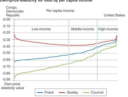
countries than for high-income countries. The Cournot and Frisch own-price

elasticities decline monotonically in absolute value from poor to rich

coun-tries. The Cournot and Frisch own-price elasticities for food are all larger

than the corresponding Slutsky elasticity. However, with rising affluence the

real income effect of a food-price change becomes increasingly smaller and

the three elasticities converge (fig. 3). The discussion that follows is limited

to the Slutsky own-price elasticity for food since it is the only measure that

did not fully perform in accordance with Timmer’s proposition.

In appendix table 3, the Slutsky own-price elasticity (equation 7) of demand

for food, beverages, and tobacco begins at -0.23 for the Congo, increases (in

absolute value) to -0.384 (Malaysia to Argentina), and declines thereafter

(absolutely) to -0.24 for the United States. To clarify the reason for this, take

15

the logarithmic derivative of equation 7, using equation 1 and suppressing

the error term:

.

(15)

If good i is a luxury,

β

i

> 0, and the derivative is negative, as real per capita

income increases, the Slutsky own-price elasticity of the good decreases.

If good i is a necessity,

β

i

< 0 so that –

β

i

> 0. If the term in brackets on the

right side of equation 15 is positive, then both the numerator and the

deriva-tive are posideriva-tive. This is the case for food, beverages, and tobacco. When

w

_ic

is sufficiently large—that is, when Q

_c

is sufficiently small—the derivative

for this good is positive for the poorest countries. Eventually, however,

w

_ic

becomes sufficiently small so that the derivative becomes negative. In this

case, the Slutsky own-price elasticity becomes smaller in absolute value. The

turning point, when the Slutsky own-price elasticity starts declining with

increasing per capita income, is at the per capita income level of Argentina—

or at 22 percent of the per capita income level of the United States.

Food Subgroups—Estimates and Elasticities

Table 4 presents the estimated parameters for the second-stage model

(equa-tion 10), the food subgroups. The estimate for K3 exceeds 1, confirming the

presence of heteroskedasticity in country group 3. The beta (

β

) estimates

for cereals, meat, fish, oils and fat, and fruits and vegetables are negative,

indicating that these food-product categories are (conditionally)

inelastic, while the remaining categories are conditionally

expenditure-elastic.

10

_{The negative beta estimates for cereals and fruits/vegetables are larger}

(in absolute value) than for the other food categories. These categories include

expenditures on grains, roots, and tubers, and both categories are particularly

sensitive to the level of affluence. Table 4 also includes the diagonal elements

(

)

(

)

(

)(

)

2

₁

log

1

i ic i i c ic ic i ic i

w

d

S

Q

w w

w

β

β

β

φ

β

β





−



+

−



=

+

−

−

10 _{The parameter estimates in table} 8 are conditional on total per capita food expenditures, not total per capita expenditures.

Figure 3

Own-price elasticity for food by per capita income

1

United States Per capita income

Low-income Middle-income High-income Congo,

Democratic Republic

1_{Countries are arranged in ascending order of affluence.}

Source: Author’s calculations using the 2005 International Comparison Program (ICP) data.

-0.90 -0.80 -0.70 -0.60 -0.50 -0.40 -0.30 -0.20 -0.10 -0.00 Own-price elasticity value

of the Slutsky matrix, which are the compensated own-price effects for each

food subgroup. These effects are all negative, satisfying the law of demand.

Marginal share estimates for each food subgroup, conditional on total food

expenditures, are plotted in figure 4 and reported in appendix table 8 by

country. These estimates measure how an additional unit of food

expendi-tures is allocated across the eight food subgroups. Figure 4 illustrates how

the marginal share for a food category varies by country based on the level

of affluence. With low-income countries, a greater portion of an additional

unit of food expenditures is allocated to cereals and fruits/vegetables, which

include staples such as corn meal and rice. As countries become more

affluent, the portion of additional food expenditures allocated to cereals

and fruits/vegetables decreases, and a greater portion is allocated to “other”

food expenditures, which includes restaurant expenditures and high-end

purchases, and beverages/tobacco. For instance, a dollar increase in food

Table 4

Maximum-likelihood estimates of the food subgroups model,

144 countries, 2005

a

Parameter Standard error Beta β*

Cereals -0.077 0.008*

Meat -0.001 0.007

Fish -0.009 0.004**

Dairy and eggs 0.002 0.004

Oils and fat -0.014 0.003*

Fruit and vegetables -0.039 0.007*

Food other 0.088 0.010*

Beverages and tobacco 0.051 0.008*

Alpha α*

Cereals 0.062 0.011*

Meat 0.143 0.010*

Fish 0.037 0.006*

Dairy and eggs 0.084 0.007*

Oils and fat 0.014 0.004*

Fruit and vegetables 0.100 0.010*

Food other 0.333 0.014*

Beverages and tobacco 0.228 0.011*

Slutsky own-price effects

π

*_ii

Cereals -0.205 0.033*

Meat -0.136 0.023*

Fish -0.102 0.012*

Dairy and eggs -0.100 0.015*

Oils and fat -0.036 0.006*

Fruit and vegetables -0.210 0.022*

Food other -0.231 0.051*

Beverages and tobacco -0.127 0.027

Heteroskedasticity measures

K2 0.851 0.019*

K3 1.090 0.013*

a_{Comoros is excluded from the analysis. Egypt and Russia were reported twice and were}

averaged for estimation. Three country groups are considered for heteroskedasticity. * and ** denote significance at the 0.01 and 0.05 level, respectively. Alpha, beta, and pi estimates are based on equations 10a−10c.

17

Figure 4

Distribution of an additional $1 of income across 144 countries, food subcategories

1

United States Per capita income

Congo, Democratic Republic 1.00

Marginal share value

.90 .80 .70 .60 .50 .40 .30 .20 .10 0

Beverages and tobacco Food other

Fruits and vegetables Oils and fats

Dairy Fish Meats Cereals

1_{Countries are arranged in ascending order of affluence.}

Source: Author’s calculations using the 2005 International Comparison Program (ICP) data.

expenditures results in cereal expenditures in the Democratic Republic of

Congo increasing by 31 cents (appendix table 8). However, cereal

expendi-tures in the United States decrease by 1.5 cents, indicating the lower status

afforded this category by most consumers in rich countries. In contrast,

expenditures on “other” food increase by only 5 cents in the Democratic

Republic of Congo, but by 42 cents in the United States.

The expenditure and price elasticities calculated using the Florida-Slutsky

model are conditional on a given food budget. In other words, the

expendi-ture elasticity measures the percentage change in demand given a percentage

change in total food expenditures, while the price elasticity measures the

percentage response given a percentage change in price assuming a given

food budget. However, the conditional elasticities can be converted to

uncon-ditional elasticities using the parameters estimated from the Florida-PI model

in the first stage, as specified by equations 11-14.

The unconditional expenditure elasticity (equation 11) measures the

percentage change in demand from a percentage change in overall income

(or total spending). The unconditional income elasticities are all less than

1, except for “other” food and beverages/tobacco in low-income countries

(appendix table 5). This is consistent with conventional theory that food is a

necessity and not a luxury item in household expenditures. Given the

rela-tively low food budget share of beverages/tobacco in many low-income

coun-tries, this category can be considered a luxury item among consumers in some

poorer countries.

Similar to the estimated income elasticity for aggregate consumption

catego-ries, the income elasticity for the food subcategories is largest in the poorer

countries and declines in magnitude with affluence. Across each country,

staple food items (with negative

*

i

β

) have smaller elasticities than the more

conditionally elastic food items such as beverages/tobacco, meat, and dairy.

For example, the income elasticity for cereals ranges from 0.69 in the

Democratic Republic of Congo to -0.09 in the United States. In contrast, the

elasticity for beverages and tobacco is higher across all countries, ranging

from 7.1 in Liberia to 0.42 in the United States.

The conditional Slutsky elasticity is given by

ε

_ijc*

=

π

_ij*

/

w

_ic*

, where

_π

*_ij

is

the conditional Slutsky price parameter in country c for good i with respect

to good j, and

_w

_ic*

is the conditional fitted budget share (at geometric

mean prices) of food group

i S

∈

_g

in country c. Since for a given food

subgroup i,

_π

*_ij

is invariant across countries, the conditional Slutsky

elas-ticity for food subgroup i will be greater for smaller budget shares. Poorer

countries typically have larger budget shares for staple items such as breads

and cereals, which form a smaller share of food budget among wealthier

countries. Therefore, contrary to theory, the estimated conditional Slutsky

own-price elasticities for cereals may be larger for wealthier countries. This

problem of a constant

_π

*_ij

continues if one calculates unconditional Slutsky

price elasticities from the conditional one using equation 13.

The unconditional Frisch own-price elasticities are not a function of

_π

_ij*

and do not suffer the problem encountered in calculating the unconditional

Slutsky elasticities. Using the estimated parameters from stage one and two

and using equation 12, Frisch own-price elasticities are calculated. These

unconditional own-price elasticities (appendix table 6) represent elasticities

estimated at a point when the marginal utility of income is held constant.

The values of the Frisch own-price elasticities lie between the values of the

Slutsky own-price elasticities—when real income is held constant—and the

Cournot own-price elasticities—when nominal income is held constant—and

can be considered a reasonable estimate of the average own-price

elastici-ties for the food subcategories. The Slutsky and Cournot elasticielastici-ties are not

estimated for these products, as their calculation using equations 13 and 14

requires the assumption of preference independence.

The Frisch own-price elasticities for the food subcategories vary by affluence

according to economic theory; consumers in low-income countries are more

responsive to price changes than are those in higher-income countries. For

instance, the value for breads and cereals ranges from 0.50 in the Democratic

Republic of Congo to 0.06 in the United States. The absolute values of the

own-price elasticities are smaller for food groups such as breads/cereals,

oils/fats, and fruits/vegetables, and particularly large for “other” foods and

beverages/tobacco. Also, low-income countries are particularly sensitive

to changes in the price of “other” food and beverages/tobacco, relative to

middle- and high-income countries. Given a 1-percent increase in the price

of “other” food, consumption in this category declines on average by more

than 1 percent in low-income countries but by less than 0.5 percent in

high-income countries.