San Jose State University
SJSU ScholarWorks
Master's Projects Master's Theses and Graduate Research
Spring 6-8-2016
Vigene
̀
re Score for Malware Detection
Suchita Deshmukh
San Jose State University
Follow this and additional works at:https://scholarworks.sjsu.edu/etd_projects Part of theInformation Security Commons
This Master's Project is brought to you for free and open access by the Master's Theses and Graduate Research at SJSU ScholarWorks. It has been accepted for inclusion in Master's Projects by an authorized administrator of SJSU ScholarWorks. For more information, please contact
Recommended Citation
Deshmukh, Suchita, "Vigenère Score for Malware Detection" (2016).Master's Projects. 487. DOI: https://doi.org/10.31979/etd.35dg-fyke
Vigenère Score for Malware Detection
A Project Presented to
The Faculty of the Department of Computer Science San Jose State University
In Partial Fulfillment
of the Requirements for the Degree Master of Science
by
Suchita Deshmukh May 2016
c
○2016
Suchita Deshmukh ALL RIGHTS RESERVED
The Designated Project Committee Approves the Project Titled
Vigenère Score for Malware Detection
by
Suchita Deshmukh
APPROVED FOR THE DEPARTMENTS OF COMPUTER SCIENCE
SAN JOSE STATE UNIVERSITY
May 2016
Dr. Mark Stamp Department of Computer Science Dr. Christopher Pollett Department of Computer Science Fabio Di Troia Department of Mathematics
ABSTRACT
Vigenère Score for Malware Detection by Suchita Deshmukh
Previous research has applied classic cryptanalytic techniques to the malware detection problem. Specifically, scores based on simple substitution cipher cryptanal-ysis and various generalizations have been considered. In this research, we analyze two new malware scoring techniques based on classic cryptanalysis. Our first ap-proach relies on the Index of Coincidence, which is used, for example, to determine the length of the keyword in a Vigenère ciphertext. We also consider a score based on a more complete cryptanalysis of a Vigenère cipher. We find that the Vigenère score is competitive with previous statistical-based malware scores.
ACKNOWLEDGMENTS
I would like to express my deep gratitude to Dr. Stamp for his valuable guidance and supervision throughout the project work. I am also grateful to my committee members for reviewing my work and providing constructive feedback. Finally, I wish to thank my husband for his support and encouragement throughout my Master’s program.
TABLE OF CONTENTS
CHAPTER
1 Introduction . . . 1
2 Previous Research . . . 4
2.1 Simple Substitution Distance Tecnique . . . 4
2.2 Simple Substitution and Column Transposition Scoring Technique 7 3 Vigenère Cipher . . . 11
3.1 Vigenère Encryption . . . 11
3.2 Vigenère Decryption . . . 13
3.3 Breaking Vigenère Cipher . . . 13
3.3.1 Kasisky Test . . . 14
3.3.2 Friedman Test . . . 15
3.4 Vigenère Cipher Score for Malware Detection . . . 17
3.4.1 Score using Index of Coincidence . . . 18
3.4.2 Score using Vigenère Cryptanalysis . . . 19
4 Experiments and Results . . . 24
4.1 Parameters . . . 24
4.2 Dataset . . . 25
4.3 Results . . . 27
4.4 Results for Varying Key Lengths . . . 30
4.5 SVM Results . . . 31
APPENDIX
A Scatter Plots and ROC curves on the basis of Index of Coinci-dence . . . 37
B Scatter Plots and ROC curves on the basis of Vigenère Cypt-analysis . . . 45
LIST OF TABLES
1 Simple Substitution Key with shift = 3 . . . 4
2 Simple Substitution Encryption . . . 5
3 Expected Digraph Distribution Matrix E . . . 6
4 Initial key . . . 6
5 Digraph Distribution Matrix D . . . 7
6 Digraph Distribution Matrix D . . . 7
7 Substitution Key . . . 8
8 Transposition Key . . . 8
9 Intermediate Ciphertext Matrix . . . 8
10 Final Ciphertext Matrix . . . 8
11 Initial ciphertext matrix . . . 9
12 Vigenère Encryption . . . 12
13 Vigenère Decryption . . . 13
14 Kasisky Algorithm . . . 15
15 Score using Index of Coincidence . . . 19
16 Cryptanalysis Subroutine . . . 20
17 findKey Function . . . 21
18 Compute 𝐸 Matrix . . . 22
19 Score using Vigenère Cryptanalysis . . . 23
20 Dataset . . . 27
LIST OF FIGURES
1 Vigenère Square. . . 12
2 Flow Diagram of the Proposed Technique. . . 18
3 No. of Opcodes vs AUC . . . 25
4 AUC Comparison . . . 28
5 NGVCK Scatter Plot . . . 29
6 NGVCK ROC . . . 29
7 Harebot ROC for lesser key length . . . 30
8 Harebot ROC for greater key length . . . 31
A.9 Cridex Scatter Plot . . . 37
A.10 Harebot Scatter Plot . . . 38
A.11 Security Shield Scatter Plot . . . 38
A.12 Smart HDD Scatter Plot . . . 39
A.13 Winwebsec Scatter Plot . . . 39
A.14 Zbot Scatter Plot . . . 40
A.15 Zeroaccess Scatter Plot . . . 40
A.16 Cridex ROC . . . 41
A.17 Harebot ROC . . . 41
A.18 Security Shield ROC . . . 42
A.19 Smart HDD ROC . . . 42
A.20 Winwebsec ROC . . . 43
A.22 Zeroaccess ROC . . . 44
B.23 NGVCK Scatter Plot . . . 45
B.24 Cridex Scatter Plot . . . 46
B.25 Harebot Scatter Plot . . . 46
B.26 Security Shield Scatter Plot . . . 47
B.27 Smart HDD Scatter Plot . . . 47
B.28 Winwebsec Scatter Plot . . . 48
B.29 Zbot Scatter Plot . . . 48
B.30 Zeroaccess Scatter Plot . . . 49
B.31 NGVCK ROC . . . 49
B.32 Cridex ROC . . . 50
B.33 Harebot ROC . . . 50
B.34 Security Shield ROC . . . 51
B.35 Smart HDD ROC . . . 51
B.36 Winwebsec ROC . . . 52
B.37 Zbot ROC . . . 52
CHAPTER 1 Introduction
Like the poor in the famous Biblical verse, malware will always be with us. Only six years after the launch of the first personal computer in 1975, the world was presented with its first computer virus. Ever since, malware has seemed unstop-pable. According to a 2014 report from Symantec, “[T]he release rate of malicious code and other unwanted programs may be exceeding that of legitimate software ap-plications [23].” According to F-Secure, “As much malware [was] produced in 2012 as in the previous 20 years altogether [5].” Malware [2] is an umbrella term for all malicious software programs. Such programs are designed to harm computer users in many ways, including stealing personal information, installing illegitimate software on their systems, reformatting hard drives and deleting files, and so on. In this paper, we use the terms viruses and malware interchangeably.
For many years, there has been an arms race between malware writers and anti-virus software. The most common and widely used anti-virus detection technique is signa-ture detection [2]. In this technique, pattern matching is used to scan for particular byte patterns that are found in viruses. If a matching pattern is found, the file is cat-egorized as malware. This is a very simple and often effective technique, but malware writers have developed various techniques aimed at defeating signature detection.
As the name suggests, the body of an encrypted virus is encrypted, which ef-fectively defeats signature detection [26]. However, the decryption routine is not encrypted, and this can be susceptible to signature scanning. As the next step in this evolution, malware authors created polymorphic [26] and metamorphic virus [9].
Like an encrypted virus, polymorphic virus also includes an encrypted body and de-cryptor code. But in addition, polymorphic malware changes the decryption routine with each new infection, making straightforward signature detection infeasible. How-ever, anti-virus can use emulation to detect polymorphic malware—at some point the malware will decrypt itself, at which point it will be vulnerable to signature detection. Metamorphic virus are sometimes said to be “body polymorphic”, since they morph the entire body of the malware with each new infection. This changes the internal structure and, if sufficiently thorough, it will defeat signature scanning. En-cryption is not necessary—and hence is not used—in metamorphic malware. Meta-morphic code can employ a wide variety of code morphing strategies [21].
Proposed malware detection mechanisms can rely on static analysis or dynamic analysis, or some combination thereof [1, 16, 19, 28]. In static analysis the necessary features are extracted without executing the code. Examples of such features include opcode sequences, entropy, and so on. As opposed to static analysis, dynamic analysis extracts features by executing (or emulating) code. Dynamic features can be used to determine aspects of the actual behavior of the code.
This research is based on static analysis of opcode sequences. We develop and analyze software similarity measures that are designed to distinguish malware code from benign code. Specifically, we focus on software similarity measures based on cryptanalysis of the Vigenère cipher. This work was inspired by similar malware research based on scores derived from simple substitution cryptanalysis [16] and a generalization [19].
This report is organized as follows. In Chapter 2, we briefly discuss previous malware detection research that is based on classic cryptanalytic techniques.
Chap-ter 3 gives a succinct overview of the Vigenère cipher and cryptanalytic techniques that are used to break the cipher. This chapter also discusses our scoring techniques that are based on the cryptanalysis of this cipher. In Chapter 4, we present our ex-periments and results. Chapter 5 concludes this report and we suggest some related future work.
CHAPTER 2 Previous Research
This chapter presents previous research [16, 19] that forms a basis for our imple-mentation of Vigenère score for malware detection. Even though the cryptanalytic techniques used in the present research and previous research are different, they are conceptually based on an idea of performing some cryptanalytic attack on cipher techniques. Hence, it is necessary to understand the previous research techniques before discussing the present research technique.
2.1 Simple Substitution Distance Tecnique
This first research technique [16] relies on a cryptanalysis of a simple substi-tution cipher to classify a malware file from a benign file. The simple substisubsti-tution cipher [20] is one of the oldest classical cipher techniques, where each plaintext symbol is encrypted with a ciphertext symbol, which is some displacement in the alphabet. It is also known as a Caesar cipher, when a plaintext symbol is encrypted using ciphertext symbol with a shift of 3. Consider an example given in Table 2 below to understand the encryption of a message using a simple substitution key given in Table 1.
Table 1: Simple Substitution Key with shift = 3
A B C D E F G H I J K L . . . S T U V W X Y Z D E F G H I J K L M N U . . . V W X Y Z A B C
The naive approach in order to cryptanalyze the simple substitution ciphertext can be an exhaustive search where an attacker has to try 287(26!/2) keys on an
Table 2: Simple Substitution Encryption
Plaintext C R Y P T O G R A P H Y Ciphertext F U B S W R J U D S K B
average to break a cipher, or a frequency analysis of ciphertext. In simple substitution distance (SSD) paper [16], a Jackobsen’s algorithm [10], which is a faster algorithm for the cryptanalysis of English ciphertext is analyzed and an analogous algorithm is implemented for malware detection problem given in [16].
In Jackobsen’s algorithm [10], initially a digraph distribution matrix 𝐸 is calcu-lated for a plaintext and a digraph distribution matrix𝐷is calculated for a ciphertext. For this initial𝐷 matrix, a score is calculated using the formula given below:
Score =∑︁|𝑒𝑖𝑗 −𝑑𝑖𝑗| (1)
Also, an initial key 𝐾 is guessed based on a frequency analysis of the ciphertext and a putaive plaintext is obtained by deciphering the ciphertext using this initial key
𝐾. Again, a matrix 𝐷 is calculated for this putaitive plaintext and a new score is computed using the formula(1). If the new score is better than the old one, the key
𝐾 is retained, else the key 𝐾 is modified by swapping its adjacent elements. With this modified key𝐾, again the ciphertext is decrypted and a matrix𝐷is recomputed and a new score is obtained. This process continues till we obtain the best score for which the best key 𝐾 is retained.
Consider an example explaining this process in detail. Suppose our alphabet set consists of only five characters such as J, G ,S V, and P. Here, J is the most frequently occurring character where as P is the least occurring character. The expected digraph distribution matrix𝐸 for the plaintext is given in Table 3. Suppose our ciphertext is “GPSSPVJPSPSVJGSPJVJGSVSPVS” and our initial key𝐾 is as shown in Table 4.
Using this initial key 𝐾, we decipher a ciphertext to obtain a putative plaintext “PGJJGSVGJGJSVPJGVSVPJSJGSJ” and calculate the digraph distribution matrix
𝐷 for this putative plaintext as shown in Table 5. We compute a score using these two matrices 𝐸 and 𝐷. According to Jackobsen’s algorithm, the key 𝐾 is modified in the next step and the score is recomputed. The key 𝐾 can be modified in the several ways. The simplest method is to swap the first two elements of the key. With this new putaitive key 𝐾, the putative plaintext obtained after decryption is “PJGGJSVJGJGSVPGJVSVPGSGJSG” and its corresponding𝐷matrix is shown in Table 6. On comparing Table 5 with Table 6, it is observed that for each modification in the key, only the rows and columns of matrix𝐷are getting swapped. Thus, instead of decrypting the ciphetext each time for a modified key, we can build matrix 𝐷once and only swap its rows and columns corresponding to the swap of the key elements. Hence, it helps in reducing the complexity of the algorithm.
Table 3: Expected Digraph Distribution Matrix E J G S V P J 2 3 0 4 1 G 1 0 2 1 2 S 1 2 1 0 0 V 1 0 0 1 1 P 1 2 0 1 0
Table 4: Initial key S P V J G J G S V P
An analogous process for computing an opcode-based similarity measure for mal-ware detection is implemented in SSD technique. In this technique, alphabet corre-sponds to opcodes that are extracted from the malware files. A model is built for a particular malware family and it is tested against an unknown file. The model is
Table 5: Digraph Distribution Matrix D J G S V P J 1 4 2 0 0 G 3 0 2 1 0 S 2 0 0 3 0 V 0 1 1 0 2 P 2 1 0 0 0
Table 6: Digraph Distribution Matrix D J G S V P J 0 3 2 1 0 G 4 1 2 0 0 S 0 2 0 3 0 V 1 0 1 0 2 P 1 2 0 0 0
treated as a original plaintext and an unknown file is treated as a ciphertext. For the complete implementation details and the results of this technique refer [16]
2.2 Simple Substitution and Column Transposition Scoring Technique
In this second research [19], a scoring algorithm is implemented based on the cryptanalysis of simple substitution and column transposition (SSCT) cipher. This is a more generalized statistical analysis technique in comparison to SSD technique [16]. The cryptanalysis algorithm for scoring relies on a more sophisticated Jackobsen’s algorithm mentioned in [29].We will first discuss the encryption process of SSCT cipher and then consider the cryptanalysis of the encrypted text to obtain the original message.
Suppose the plaintext we want to encrypt is “ATTACKATDAWN” and the sub-stitution key and the transposition key are shown in Table 7 and Table 8 respec-tively. After applying the substitution key in Table 7, the intermediate ciphertext is
“DWWDFNDWGDZQ”. This intermediate ciphertext is arranged in the matrix shown in Table 9. Using a transposition key, the final ciphertext “WDWFDNWDGZDQ” is obtained from the intermediate ciphertext. The final ciphertext is then constructed by reading the characters row-wise from the matrix given in Table 10.
Table 7: Substitution Key
A B C D E F G H I J K L . . . S T U V W X Y Z D E F G H I J K L M N U . . . V W X Y Z A B C
Table 8: Transposition Key 2 1 3
Table 9: Intermediate Ciphertext Matrix D W W
D F N D W G D Z Q
Table 10: Final Ciphertext Matrix W D W
F D N W D G Z D Q
Now to obtain the original message from the SSCT ciphertext, an efficient crypt-analysis algorithm outlined in [29] is used. The fundamental difference between SSD and SSCT is that, in SSD the plaintext and the ciphertext are continuous stream of characters while in SSCT the plaintext and the ciphertext are stored in the matrix form. Suppose initial ciphertext matrix is as shown in Table 11. Then, we need to compute digraph frequencies for every column based on the transposition key. Also,
when this initial matrix is unwounded, the last element of row𝑖 becomes adjacent to the first element of row 𝑖+ 1. Hence, for a given transposition key,
𝐾 = (𝑘1, 𝑘2, 𝑘3, ...𝑘𝑛)
the digraph distribution matrix D is given by
𝐷=𝐷𝑘1,𝑘2+𝐷𝑘2,𝑘3+· · ·+𝐷𝑘𝑛−1,𝑘𝑛+𝐷𝑘𝑛,𝑘1′
Here 𝐷𝑖,𝑗 is the digraph frequencies matrix when column 𝑗 is next to column 𝑖 and
𝐷𝑖,𝑗′ accounts for the digraph frequencies for the wrap around case. The required data
structure to store all these individual matrices is mentioned in [29]. If a Jakobsen’s algorithm mentioned in [10] is applied directly in this scenario, then for each loop, rows and columns of each individual 𝐷𝑖,𝑗 matrix needs to be swapped. This leads to
an increased time and space complexity. To avoid this, a smart approach is discovered in [29], where instead of swapping rows and columns of an individual𝐷𝑖,𝑗 matrix, rows
and columns of 𝐸𝑖,𝑗 matrix are swapped that yields the same score computed using
formula(1). Thus, the score is obtained by swapping rows and columns of𝐸𝑖,𝑗 matrix
increasing an efficieny of an algorithm.
Table 11: Initial ciphertext matrix
⎡ ⎢ ⎢ ⎢ ⎣ 𝑐11 𝑐12 𝑐13 . . . 𝑐1𝑛 𝑐21 𝑐22 𝑐23 . . . 𝑐2𝑛 .. . ... ... . . . ... 𝑐𝑚1 𝑐𝑚2 𝑐𝑚3 . . . 𝑐𝑚𝑛 ⎤ ⎥ ⎥ ⎥ ⎦
In SSCT [19] scoring technique, the above mentioned process is applied to calcu-late a score that classifies a malware file form a benign file. Like SSD [16] technique,
in this method also opcodes are mapped to English alphabets and an analogous algo-rithm mentioned in [29] is implemented. The complete account of this method with the results is outlined in [19].
CHAPTER 3 Vigenère Cipher
Monoalphabetic substitution ciphers such as simple substitution cipher are easily vulnerable to a frequency analysis attack [20]. This weakness of monoalphabetic sub-stitution ciphers leads to the idea for designing a polyalphabetic cipher by Alberti [17]. He suggested that in order to make ciphertext more secure against potential cryptan-alytic attacks, use two or more cipher alphabet and also switch between them during encipherment. Alberti’s idea was converted into a more practical cipher by a French diplomat, Vigenère and hence the name “Vigenère Cipher.” Vigenère cipher [17] is a form of polyalphabetic substitution ciphers. Since Vigenère cipher overcome the weakness in simple substitution cipher, it is considered to be stronger than Simple Substitution cipher. It generates an encrypted text as an interwoven series of many simple substitution ciphertexts thus disguising frequency statistics. And hence, this has remained unbreakable for over three centuries, therefore it is also known as le chiffre indéchiffrable (indecipherable). In Vigenère cipher, every letter in an alpha-betic plaintext (message) is encrypted using a different shift that corresponds to a corresponding letter in the keyword. This approach ensures one extra level of secu-rity as compared to Simple Substitution where every letter in a message is encrypted using the same shift.
3.1 Vigenère Encryption
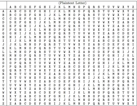
To encrypt a plaintext message, a Vigenère square that is a 26×26 matrix is used. The Vigenère square is shown in Figure 1. Each column index represents a plaintext letter and each row index corresponds to a keyword letter.
Figure 1: Vigenère Square.
The encryption process is described using an example given in Table 12. In this example, the keyword used for encryption is “LEMON.” This keyword is repeated the length of the plaintext. A ciphertext letter L is obtained as an intersection of row index that corresponds to keyword letter L and column index that corresponds to plaintext letter A. In a similar fashion, all other letters of the plaintext are encrypted. This example shows that every plaintext letter is encrypted using a different shift. Since Vigenère cipher can easily disguise the frequency of appearance of letters, it is more secure than Simple Substitution cipher.
Table 12: Vigenère Encryption
Plaintext A T T A C K A T D A W N Key L E M O N L E M O N L E Ciphertext L X F O P V E F R N H R
3.2 Vigenère Decryption
The decryption process is exactly opposite to the encryption process. In this process using a Vigenère square shown in Figure 1, a plaintext letter is retrieved by fetching a row having a keyword letter as row index and a ciphertext letter in it. Thus, the column index corresponding to the position of a cipher text letter in this row provides a plaintext letter. See the example given in Table 13. Thus, to obtain
Table 13: Vigenère Decryption
Ciphertext L X F O P V E F R N H R Key L E M O N L E M O N L E Plaintext A T T A C K A T D A W N
a plaintext letter A first search for a row with row index L and within that row for letter L, then find the corresponding column index. This column index represents plaintext letter A. Similarly, the rest of the plaintext letters are obtained.
3.3 Breaking Vigenère Cipher
Although Vigenère cipher resisted any attack for almost three centuries, it was broken because of the repetitive nature of its key used during encipherment. Like any other polyalphabetic cipher, Vigenère cipher can hide natural letter frequencies for plaintext letters. Hence, it is not very obvious to directly use frequency analysis for cryptanalysis like simple substitution ciphers. It is difficult to draw any conclusions about possible occurrence of plaintext letters. This is because, unlike simple substi-tution cipher, the same plaintext letter gets enciphered as different ciphertext letter at various points in the original message . For example if P is the most frequently occurring letter in the ciphertext, then it will not represent E in the plaintext in case of Vigenère cipher. This is because E can be encrypted as different cipher letters each
time.
In order to break Vigenère cipher, first find the key length, then divide the ciphertext into those many number of columns and finally use frequency analysis to solve an individual column, that is a simple shift cipher. With this process one can recover an original key that can be used to decipher the ciphertext. There are two methods to determine the length of the key: Kasisky test and Friedman test.
3.3.1 Kasisky Test
This method [17, 4] takes benefit of the fact that the repeated plaintext segments may be encrypted using the same keyword letters, if they occur at the distance 𝑑. Here 𝑑≡0( mod 𝑚), where 𝑚 is the length of key. The algorithm for this method is as follows:
1. In a given ciphertext, search for pairs of identical words with length at least three.
2. Calculate the distance between the two identical words as 𝑑1, 𝑑2,..., 𝑑𝑛.
3. Determine key length 𝑚 as 𝑚 divides gcd(𝑑1, 𝑑2, ..., 𝑑𝑛).
Consider the example in Table 14 to understand this method. Table 14 shows that the distance between the identical words in the ciphertext is 8. Thus, according to the algorithm, the most likely key length is 4. This method can produce more accurate key length if the ciphertext used is sufficiently large so that there are more occurrences of the identical words.
Table 14: Kasisky Algorithm
Key K I N G K I N G K I N G K I N G K I N G K I N G Plaintext T H E S U N A N D T H E M A N I N T H E M O O N Ciphertext D P R Y E V N T N B U K W I A O X B U K W W B T
3.3.2 Friedman Test
This method [7] is based on the index of coincidence. The index of coincidence determines the probability that the two randomly selected letters from the string x, having n letters are identical. This test makes use of unevenness of the letter frequencies in the cipher text to break the cipher. The index of coincidence (𝐼𝐶) is given by formula below:
𝐼𝐶 = 𝑐 ∑︁ 𝑖=1 𝑛𝑖(𝑛𝑖−1) 𝑁(𝑁 −1)/𝑐 (2)
Here, 𝑛𝑖 is the frequency of occurrence of a particular letter in the text
𝑁 is the length of the text
𝑐is the total number of alphabet. for example 𝑐= 26 for English
Further, the approximate key length is determined by a formula given as follows:
𝐾𝑝−𝐾𝑟
𝐾𝑜−𝐾𝑟
(3) Here, 𝐾𝑝 is the kappa plaintext. For English 𝐾𝑝 = 0.067, if the underlying plaintext
for the ciphertext is English
𝐾𝑟 is the kappa random. For English𝐾𝑟 = 0.0385, if the underlying plaintext for the
ciphertext is some random text
𝐾𝑜 is the 𝐼𝐶 calculated using Formula 2
In the context of the English language, if the 𝐼𝐶 of the ciphertext under con-sideration is close to 0.067 (𝐾𝑝 for English), then the underlying plaintext for this
to 0.0385 (𝐾𝑟 for English), then the underlying plaintext for this ciphertext is some
random text. Note that this method only gives approximate key length. To obtain more accurate key length ciphertext should be sufficiently large.
Once the key length is determined using either of the above methods, the actual key is recovered using frequency analysis and correlation [20]. The correlation 𝜒 is a given by the following formula:
𝜒=
𝑐 ∑︁
𝑖=1
𝑛𝑖𝑓𝑖 (4)
Here, 𝑛𝑖 is the letter frequencies for the observed column
𝑓𝑖 is the relative letter frequencies for English
𝑐is the total number of alphabet. for example 𝑐= 26 for English The algorithm to obtain key is as follows:
1. Divide the ciphertext into same number of columns as the key length.
2. For each individual column, try out Caesar cipher decryption for all 26 (A-Z) possible shifts.
3. Select a shift that produces highest correlation between letter frequencies for the decrypted column and the relative letter frequencies for the normal English text. This shift corresponds to a letter in a key.
4. Repeat step 2 and 3 for all remaining key letters.
5. Once the actual key is found, we can decrypt the ciphertext message using decryption method mentioned above.
The above algorithm was initially implemented for English ciphertext to test its efficacy. We have experimented with varying key lengths and varying sizes of
ciphetext. It is observed that in order to completely recover the plaintext from ci-phertext for a particular key length, each column of the cici-phertext matrix should at least contain 30 characters. For example, for a key “boxfish” of length 7, we obtained a correct plaintext for a ciphertext of size 230 characters.
3.4 Vigenère Cipher Score for Malware Detection
This section describes the complete implementation of the scoring technique used for the malware detection. The proposed techniques is shown in Figure 2. The implementation involves two steps. The first step is computing key length with the help of the index of coincidence technique [7]. This key length is used in the second step to recover the key and decrypt the ciphertext to give putative plaintext using this recovered key. The digraph distribution of this putative plaintext is used in the scoring part that tells whether a particular file is malware or not. Before discussing the above mentioned steps, it is necessary to talk about the process that involves generation of alphabetic ciphertext from opcode sequence of a malware or benign file.
We will consider the opcode sequence from the known virus files as plaintext and the opcode sequence from an unknown virus files as ciphertext. We will refer to all virus files of the same family as model and unknown files to score as sample. After extracting the opcodes from the virus files, these opcodes are mapped to the English alphabet depending on the computed monograph statistics of a particular malware family. Thus, the ciphertexts and plaintexts consist of the English alphabet. The details about opcode extraction process, choice of 26distinct opcodes and opcode to alphabet mapping can be found in Chapter 4 under Experiments and Results.
Figure 2: Flow Diagram of the Proposed Technique.
3.4.1 Score using Index of Coincidence
This is the first step that involves the computation of index of coincidence (𝐼𝐶) for a model and various test samples which is further given to scoring function. 𝐼𝐶
for a model is referred as familyIC whereas 𝐼𝐶 for a sample is referred as 𝐼𝐶. The formula for computing 𝐼𝐶 is given in (2). In order to compute familyIC, first a set of all opcodes for all virus files in that family is obtained. Thus, according to
𝐼𝐶 formula(2), 𝑛𝑖 is frequency of occurrence of a particular opcode in that set and
𝑁 is total number of opcodes in the set. In a similar way, for an unknown file,
𝐼𝐶 is calculated. In case of an unknown file, 𝑛𝑖 is frequency of occurrence of a
particular opcode in that file and 𝑁 is the length of that file. Then a score function is implemented as given in Table 15 that classifies a sample as malware or not. Also, the obtained score is used as a key length in step 2 that is explained in the next
section.
Table 15: Score using Index of Coincidence Algorithm Parameters:
familyIC- Expected IC for a particular malware family IC- Calculated IC for a test sample
score=|familyIC−IC|
if score ≤ threshold
unknown file is a virus of the same family else
unknown file is not a virus of the same family end if
3.4.2 Score using Vigenère Cryptanalysis
This is the second step that involves implementation of a scoring technique based on the cryptanalysis [4] of ciphertext of test samples. The ciphertext for test samples is assumed as some form of Vigenère encryption. This ciphertext is the opcode sequence in the form of the English alphabet. This ciphertext along with its key length that is obtained in section 3.4.1 is provided to a cryptanalysis subroutine given in Table 16. The complete process for scoring a test sample is given below.
1. Generate ciphertext for a test sample in the form of the English alphabet. 2. Input the generated ciphertext and key length obtained using index of
coin-cidence to a cryptanalysis subroutine given in Table 16 .This cryptanalysis subroutine has a findKey and decrypt functions that gives key and putative plaintext respectively. The findKey function is given in Table 17.
3. Compute normalized digraph distribution matrix E for original plaintext for a model. The method is explained in Table 18.
4. Compute normalized digraph distribution matrix D for putative plaintext. The process for computation of matrix D is same as matrix E. Both the matrices E and D are normalized to avoid sparse matrices.
5. Input E and D matrices to a scoring function explained in Table 19. 6. This score determines whether a test sample is malware or not.
Table 16: Cryptanalysis Subroutine Algorithm Parameters:
ciphertext, keyLength, putativePlaintext, key
if keyLength≤0
putativePlaintext=ciphertext else
key=findKey(ciphertext,keyLength)
Table 17: findKey Function Algorithm Parameters:
ciphertext, keyLength, putativePlaintext, key
FreqAlphaMapping - HashMap with alphabets as key and count of alphabets as value monostat - monograph statistics for a particular malware family
Initialize key to 0
Initialize monostat to opcode frequences Initialize row to 𝑙𝑒𝑛𝑔𝑡ℎ(ciphertext)/keyLength Initialize col to keyLength
CT=generateCipherMatrix(ciphertext,row,col)
for each column in CT
freqCount=freq(column) end for for 𝑖= 0 to 25 FreqAlphaMapping.put(65+𝑖, freqCount[𝑖]) end for sort(FreqAlphaMapping) Initialize maxCorr to 0 while loop<26 corr = 0.0 𝑐= 65 + loop for 𝑗 = 0 to 25
𝑑= (FreqAlphaMapping[𝑗].alpha−𝑐+ 26) mod 26
corr=FreqAlphaMapping[𝑗].count * monostat[𝑑]
end for if corr>maxCorr 𝑚= loop maxCorr=corr end if next loop end while key+ =m+ 65 end for
Table 18: Compute 𝐸 Matrix Algorithm Parameters:
Plaintext- Alphabetical plaintext generated for malware family
normFactor- One dimensional array holding total occurrences of opcodes per row
𝐸 Matrix- Normalized digraph distribution matrix for malware family
Initialize 𝐸 to 0
for 𝑖= 1 to Length of plainetxt
𝐸[Plaintext.𝑐ℎ𝑎𝑟𝐴𝑡(𝑘−1)−65][Plaintext.𝑐ℎ𝑎𝑟𝐴𝑡(𝑘)−65]+ = 1 end for for 𝑗 = 1 to 26 for 𝑘 = 1 to 26 normFactor[𝑗]+ =𝐸[𝑗][𝑘] end for end for for 𝑖= 1 to 26 for 𝑗 = 1 to 26 if normFactor[𝑖] ̸= 0 𝐸[𝑖][𝑗] =𝐸[𝑖][𝑗]/normFactor[𝑖] end if end for end for
Table 19: Score using Vigenère Cryptanalysis Algorithm Parameters:
𝐸 Matrix- Normalized digraph distribution matrix for malware family
𝐷 Matrix- Normalized digraph distribution matrix for test sample
for 𝑖= 1 to 𝑛 for 𝑗 = 1 to 𝑛 score[𝑖][𝑗] =|𝐸[𝑖][𝑗]−𝐷[𝑖][𝑗]| score+ =score[𝑖][𝑗] end for end for if score ≤ threshold
unknown file is a virus of the same family else
unknown file is not a virus of the same family end if
CHAPTER 4 Experiments and Results
This chapter illustrates the experiments and the results obtained via implementa-tion of the scoring algorithm in Java. Initially, the gathered executable files from both malware and benign dataset were disassembled using ollydbg [14]. Then the opcodes from these disassembled files were extracted using GivemeASM3.jar. The various malware families used for experimentation and the results of these experiments are explained in the subsequent sections.
4.1 Parameters
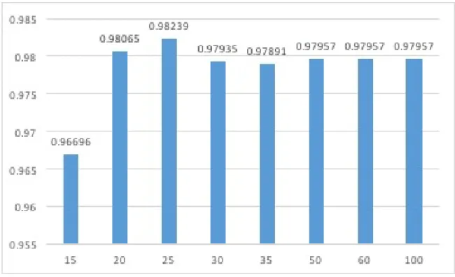
It is mentioned in [15] that there are more than 130 opcodes in any particular processor. Thus, if a matrix is constructed for scoring using such opcodes, it will be too large to compare. Moreover, only a subset of opcodes out of all such opcodes contributes to a particular behavior of a file, that is either malicious or benign. Hence, it is appropriate to choose only frequently occurring opcodes and put all non-frequent opcodes into “other” category to build 𝐸 and 𝐷 matrices for scoring. To come up with such topmost occurring opcodes, an experiment was conducted over 643 files from Zbot, Winwebsec and Cygwin datasets. The purpose of this experiment was to choose top𝐾 opcodes which contribute to most of the functionality. A graph given in Figure 3 is plotted between number of opcodes on X-axis and AUC values on Y-axis to find such𝐾 opcodes. It was seen from the Figure 3 that 𝐾 = 25 gives the highest AUC value. Thus, in both of the above mentioned approaches, total 26 opcodes were used to conduct experiments. These 26 opcodes consists of 25 frequently occurring opcodes and all non frequently occurring opcodes grouped into “other" category.
Figure 3: No. of Opcodes vs AUC
4.2 Dataset
The dataset used for this project consists of malware dataset and benign dataset. The malware dataset includes various malware families such as Next Generation Virus Generation Kit (NGVCK), Harebot, Zeroaccess, Zbot, Security Shield, Winwebsec, Smart HDD, Cridex. These families are described succinctly below:
∙ NGVCK [25] is a metamorphic virus that replicates itself using code morphing techniques such as subroutine reordering and dead code insertion.
∙ Harebot is a windows rootkit that opens up the user system to remote hackers allowing them to perform malicious activities.
∙ Zeroaccess is a trojan horse that mainly infects Microsoft Windows OS. It down-loads other malware on an infected computer system with the help of botnets
that are mainly used in bitcoin mining and click frauds.
∙ Zbot [24] is also known as Zeus, designed to carry out malicious and criminal tasks such as stealing banking information of users using techniques such as form grabbing and keystroke logging.
∙ Security Shield [11] is a variant of Win32/Winwebsec family that generates fake warnings about nonexistent threats and asks users to register to paid software to remove these threats.
∙ Winwebsec [12] is a type of malicious software that targets Windows users. It generates fake alerts and detections in order to convince users to purchase illegitimate software that impersonates legitimate anti-virus software.
∙ Smart HDD is a malicious program that represents itself as a hardware mon-itoring system and generates misleading warning for hard drive failures and memory errors.
∙ Cridex [13] is a trojan that adds the compromised system to the network of botnets and injects itself into victim’s web browser to collect confidential infor-mation such as banking credentials.
Since all the above mentioned malicious programs are mainly designed for win-dows platform, it is logical to use benign files belonging to the same environment for scoring. Thus the benign dataset used consists of Cygwin utility files. The Table 20 shows total number of files in the malware and benign dataset. Since there are fewer number of files in each dataset, we performed a five-fold cross validation to get most out of it. We divided each malware dataset into five sets; four out of five sets are used
for training and the remaining one set is used for testing. This process is repeated five times, each time selecting different sets for training and testing.
Table 20: Dataset NGVCK 200 Harebot 54 Zeroaccess 230 Zbot 242 Security Shield 59 Winwebsec 161 Smart HDD 69 Cridex 75 Cygwin 40 4.3 Results
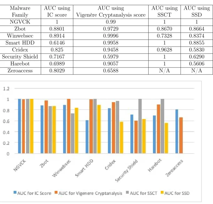
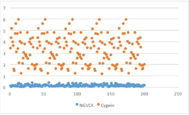
The similarity scores obtained using the scoring algorithms mentioned in Chap-ter 3 for the comparison of various malware families with virus files in the same family and the benign files are described in this section. The results are shown in terms of AUC values. The AUC values [3] are obtained by plotting Receiver Operating Curve (ROC). The ROC [6] is a plot between false positive rate on the X-axis and true positive rate on the Y-axis. The accuracy of our detection system is calculated using AUC that is an area under ROC curve. Table 21 shows comparison between our detection system and previous research. Graphically this comparison is shown in Graph 4. It can be seen from Graph 4 that our detection system performed better in case of malware families such as NGVCK, Zbot and Smart HDD. In case of an NGVCK malware family, Scatter plot in Figure 5 reveals a clear distinction between malware files and benign files. In Figure 5, the blue solid dots corresponds to malware files where as orange solid dots corresponds to benign files. Hence, we got an AUC of perfect one for NGVCK which is an ideal condition and is shown in ROC curve in
Table 21: Results
Malware AUC using AUC using AUC using AUC using Family IC score Vigenère Cryptanalysis score SSCT SSD
NGVCK 1 0.99 1 1 Zbot 0.8801 0.9729 0.8670 0.8664 Winwebsec 0.8914 0.9996 0.7328 0.8374 Smart HDD 0.6146 0.9958 1 0.8855 Cridex 0.825 0.9458 0.9628 0.5830 Security Shield 0.7167 0.5979 1 0.6290 Harebot 0.6989 0.9057 1 0.5606 Zeroaccess 0.8029 0.6588 N/A N/A
Figure 4: AUC Comparison
Figure 6. For Zbot, the AUC value is better than both previous research techniques. In case of Smart HDD, the AUC value is closer to AUC value of SSCT technique but better than AUC value of SSD technique. In almost all cases, our technique is performing better than the SSD technique and in some case it reaches closer to SSCT technique as mentioned above. We tested our detection system for one more family,
Figure 5: NGVCK Scatter Plot
Figure 6: NGVCK ROC
Zeroaccess, which is not considered in SSCT and SSD techniques. Even though the results obtained for this family are not very good, we have still included them in our result set for comparison in the future. For better visualization of the results, the scatter plots and ROC curves for the rest of the malware families for both scoring
algorithms are given in the Appendices A and B.
4.4 Results for Varying Key Lengths
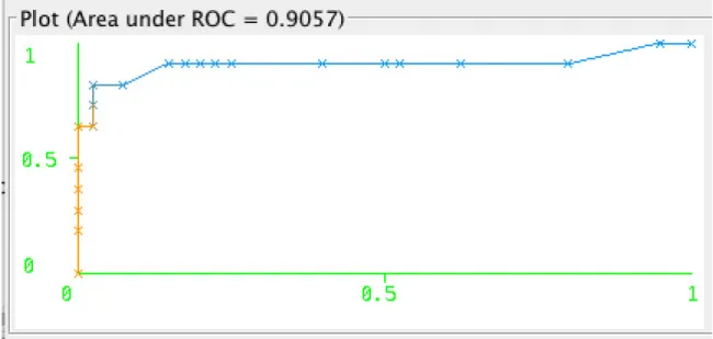
We know that our approach II scores are dependent on the key lengths obtained during approach I. These are approximate key lengths and thus we wanted to check if varying the key lengths can improve the approach II scores. We experimented on harebot malware family since it can be an interesting case to see if its auc value improves from 0.9057. We used the key length one lesser as well as one greater than the actual key length for all harebot test samples. The results of these experiments are shown in Figure 7 and Figure 8. It is observed that there is no change in the auc value when the key length is greater than the actual key length and it slightly improved when the key length is lesser that the actual key length. Moreover, the same experiments can be conducted for the remaining malware families under consideration in the future.
Figure 8: Harebot ROC for greater key length
4.5 SVM Results
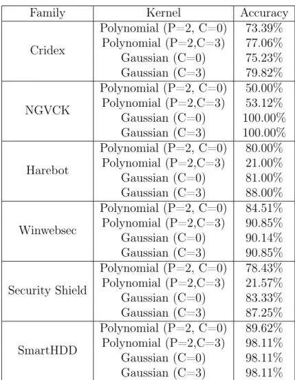
SVM [22] is an acronym for support vector machine, is used as a binary classifier. It is a supervised learning technique that means it needs labelled data. Due to the fact that SVM acts as a classification technique, it is very natural to apply the technique to a set of scores, as opposed to a raw data itself. Hence although, it is a challenging task to determine a good technique to combine scores to build a strong score, SVM is a reasonable technique to combine such scores rather than using an ad hoc score combination. Therefore, in our case we used SVM to combine our approach I and approach II scores. We tested two kernel functions such as polynomial and Gaussian with different parameters to determine the accuracy of our classification technique. The results for our experiments is shown in Table 22. In the Table 22, the parameters P and C are known as the degree of a polynomial learning function and the trade-off between a training error and a margin respectively. It is observed that a gaussian kernel function with parametr C=3 gives a better accuracy in all cases.
Table 22: SVM Results
Family Kernel Accuracy Cridex Polynomial (P=2, C=0) 73.39% Polynomial (P=2,C=3) 77.06% Gaussian (C=0) 75.23% Gaussian (C=3) 79.82% NGVCK Polynomial (P=2, C=0) 50.00% Polynomial (P=2,C=3) 53.12% Gaussian (C=0) 100.00% Gaussian (C=3) 100.00% Harebot Polynomial (P=2, C=0) 80.00% Polynomial (P=2,C=3) 21.00% Gaussian (C=0) 81.00% Gaussian (C=3) 88.00% Winwebsec Polynomial (P=2, C=0) 84.51% Polynomial (P=2,C=3) 90.85% Gaussian (C=0) 90.14% Gaussian (C=3) 90.85% Security Shield Polynomial (P=2, C=0) 78.43% Polynomial (P=2,C=3) 21.57% Gaussian (C=0) 83.33% Gaussian (C=3) 87.25% SmartHDD Polynomial (P=2, C=0) 89.62% Polynomial (P=2,C=3) 98.11% Gaussian (C=0) 98.11% Gaussian (C=3) 98.11%
CHAPTER 5
Conclusions and Future Work
We modeled and implemented an opcode-based static analysis technique for mal-ware detection. This technique uses a scoring algorithm based on cryptanalysis of Vigenère cipher [4]. We built a training model from a dataset of various malware families mentioned in Section 4.2 and tested this model against virus files from the same malware family as well as benign files. We tested our scoring algorithm on wide range of malware families in order to analyze their reaction for our scoring technique. This algorithm proves to be efficient in almost all cases of malware families as com-pared to SSD. In comparison to SSCT, our algorithm performed better in case of NGVCK, Zbot and Smart HDD. Thus, for a particular threshold value, our detection technique effectively classifies a malware file from a benign file.
Presently, our detection system is only able to distinguish a malware file from a benign file. In future, this detection technique can be modified to classify a test file to a particular malware family it belongs based on higher level calculations of index of coincidence values. Also, in this project morphed variants of the virus files are not analyzed. This could be a future scope, where one can build a morphing engine [18] to create a morphed variants of virus files using the dataset used in this project and analyze how our technique performs. Although, our second scoring technique based on complete Vigenère cryptanalysis is performing better than the SSD technique, it is not doing well compared to the SSCT technique in all the malware families. Hence, in future our approach II scores can be improved by implementing an automated approach which will consider varying key lengths, as opposed to only approximate key lengths, which are presently used.
LIST OF REFERENCES
[1] C. Annachatre, T. H. Austin, M. Stamp, Hidden Markov Models for Malware Classification, Journal of Computer Virology and Hacking Techniques, 11(2):59– 73, May 2015
[2] J. Aycock,Computer Viruses and Malware, Springer, 2006
[3] A. P. Bradley, The Use of the Area Under the ROC Curve in the Evolution of Machine Learning Algorithms, Pattern Recognition, 30:1145–1159, 1997
[4] Cryptanalysis of Vigenère Cipher and Substitution Cipherhttp://shodhganga. inflibnet.ac.in/bitstream/10603/26543/10/10_chapter5.pdf
[5] F-Secure Annual Security Report 2007, https://www.f-secure.com/ documents/10192/1118990/AnnualReport_2007_en.pdf/
[6] T. Fawcett, An Introduction to ROC Analysis, Pattern Recognition Letters, 27(8):861–874
[7] W. F. Friedman, The index of coincidence and its applications in cryptography, Aegean Park Press, 1987
[8] C. Hosmer, Polymorphic and Metamorphic Malware, https://www.blackhat. com/presentations/bh-usa-08/Hosmer/BH_US_08_Hosmer_Polymorphic_ Malware.pdf
[9] Hunting for Metamorphic https://www.symantec.com/avcenter/reference/ hunting.for.metamorphic.pdf
[10] T. Jakobsen, A fast method for the cryptanalysis of substitution ciphers, Cryp-tologia, 19:265–274, 1995
[11] Microsoft Malware Protection Center, SecurityShield, http://www. microsoft.com/security/portal/threat/encyclopedia/Entry.aspx? Name=SecurityShield
[12] Microsoft Malware Protection Center, Winwebsec, https://www.microsoft. com/security/portal/threat/encyclopedia/entry.aspx?Name=Win32% 2fWinwebsec
[13] Microsoft Malware Protection Center, Cridex, http://www.microsoft.com/ security/portal/threat/encyclopedia/entry.aspx?Name=Win32%2FCridex
[14] OllyDbg http://www.ollydbg.de/
[15] N. Runwal, R Low, and M. Stamp, Opcode graph similarity and metamorphic detection Journal of Computer Virology and Hacking Techniques, 8(2):37–52, 2012
[16] G. Shanmugam, R. M. Low, and M. Stamp, Simple substitution distance and metamorphic detection, Journal of Computer Virology and Hacking Techniques, 9(3):159–170, 2013
[17] S. Sing, The code book: the science of secrecy from ancient Egypt to quantum cryptography, Anchor, 2011
[18] S. M. Sridhara, Metamorphic worm that carries its own morphing en-gine, http://citeseerx.ist.psu.edu/viewdoc/download?doi=10.1.1.344. 549&rep=rep1&type=pdf, 2012
[19] S. Srinivasan, SSCT Score for Malware Detection, Master’s report, Department of Computer Science, San Jose State University, 2015,
http://scholarworks.sjsu.edu/etd_projects/444/
[20] M. Stamp and R. M. Low, Applied Cryptanalysis: Breaking Ciphers in the Real World, Wiley, 2006
[21] M. Stamp,Information Security: Principles and Practice, second edition, Wiley, 2011
[22] M. Stamp, Machine Learning with Applications in Information Security, first edition, unpublished manuscript, 2015
[23] Symantec Annual Security Report 2008,http://www.realwire.com/releases/ symantec-announces-messagelabs-intelligence-2008-annual-security-report
[24] Symantec Security Response, ZBOT, http://www.symantec.com/security_ response/writeup.jsp?docid=2010-011016-3514-99
[25] P. Szor, The Art of Computer Virus Research and Defense, Pearson Eduction, 2005
[26] Understanding and Managing Polymorphic viruses https://www.symantec. com/avcenter/reference/striker.pdf
[27] H. Van Tilborg, An introduction to cryptology, Springer Science and Business Media, Vol. 52, 2012
[28] S. Vemparala, Malware Detection Using Dynamic Analysis,Master’s report, De-partment of Computer Science, San Jose State University, 2015,
http://scholarworks.sjsu.edu/etd_projects/403/
[29] J. Yi, Cryptanalysis of Homophonic Substitution-Transposition Cipher, Depart-ment of Computer Science, San Jose State University, 2014,
APPENDIX A
Scatter Plots and ROC curves on the basis of Index of Coincidence
In this section, we present the scatter plots and ROC curves for the various malware families scored on the basis of Index of Coincidence. When performing the experiments on the malware families mentioned in Section 4.2, we stored the malware and benign scores in .txt files and used these score to plot scatter plots as shown in Figures A.9 − A.15. Using these score, we further calculated true positive and false negative rates to generate ROC curves given in Figures A.16 − A.22 to obtain AUC values.
Figure A.10: Harebot Scatter Plot
Figure A.12: Smart HDD Scatter Plot
Figure A.14: Zbot Scatter Plot
Figure A.16: Cridex ROC
Figure A.18: Security Shield ROC
Figure A.20: Winwebsec ROC
APPENDIX B
Scatter Plots and ROC curves on the basis of Vigenère Cyptanalysis
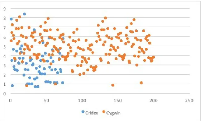
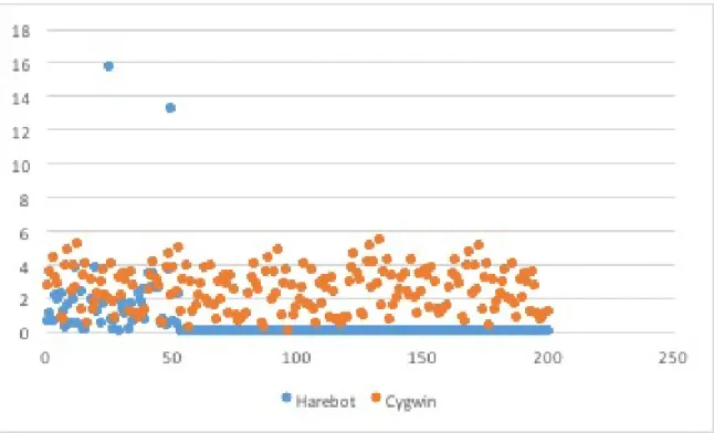
In this section, we present the scatter plots and ROC curves for the various malware families scored on the basis of Vigenère Cyptanalysis. The scatter plots are shown in Figures B.23 − B.30 and ROC curves are given in Figures B.31− B.38.
Figure B.24: Cridex Scatter Plot
Figure B.26: Security Shield Scatter Plot
Figure B.28: Winwebsec Scatter Plot
Figure B.30: Zeroaccess Scatter Plot
Figure B.32: Cridex ROC
Figure B.34: Security Shield ROC
Figure B.36: Winwebsec ROC