by
Jacob Bradley Kenyon
Thesis presented in partial fullment of the requirements for
the degree of Master of Commerce (Statistics) in the
Department of Statistics and Actuarial Science at
Stellenbosch University
Supervisor: Dr. David Hofmeyr
Declaration
By submitting this thesis electronically, I declare that the entirety of the work contained therein is my own, original work, that I am the sole author thereof (save to the extent explicitly otherwise stated), that reproduction and pub-lication thereof by Stellenbosch University will not infringe any third party rights and that I have not previously in its entirety or in part submitted it for obtaining any qualication.
April 2019
Date: . . . .
Copyright©2019 StellenboschUniversity Allrightsreserved
Abstract
Improving Hyperplane Based Density Clustering
Solutions With Applications in Image Processing
J. B. Kenyon
Department of Statistics and Actuarial Science, University of Stellenbosch,
Private Bag X1, Matieland 7602, South Africa.
Thesis: MCom (Statistics)
April 2019
Minimum Density Hyperplane (MDH) clustering is a recently proposed method that seeks the location of an optimal low-density separator by directly min-imising the integral of the empirical density function on the separating surface. This approach learns underlying clusters within the data in an ecient and scalable way using projection pursuit. The main limitation of MDH is that it denes clusters using a linear hyperplane. In recent research, MDH was applied to data which was non-linearly embedded in a high-dimensional feature space using Kernel Principal Component Analysis. While this method has shown to be an eective approach that extends the linear plane to a non-linear form, it does not scale well. A procedure is needed that can improve the hyperplane solution in an ecient way. We pose a novel approach to improve upon MDH by reassigning observations in a neighbourhood around a hyperplane solution using a gradient ascent procedure, Mean Shift. While Mean Shift is shown to provide promising results, the computation required to reassign objects becomes prohibitive as the size of the dataset increases. To reduce compu-tation, a single step gradient heuristic is proposed whereby observations are reassigned based on the initial gradient evaluated at each point in relation to the hyperplane. This study critically reviews the validity of these approaches through applications with simulated and real-world datasets, with a focus on applications in image segmentation. We show that these approaches have the potential to improve hyperplane solutions.
Opsomming
Verbetering na Minimum Digtheidsbasis-Klustering:
'n Toepassing in Beeldsegmentasie
J. B. Kenyon
Departement Statistiek en Aktuariële Wetenskap, Universiteit van Stellenbosch,
Privaatsak X1, Matieland 7602, Suid Afrika.
Tesis: MCom (Statistiek)
April 2019
Minimum Digtheid Hipervlak (MDH) tros-vorming is `n onlangs voorgestelde metode waartydens die optimale ligging van ?n lae digtheids-hipervlak gevind word deur die integraal van die empiriese dightheidsfunksie oor die hipervlak oppervlak te minimimeer. Hierdie benadering maak gebruik van projeksie-najaging om op `n doeltreende wyse onderliggende trosse te identiseer. Die primêre beperking van MDH is dat trosse deur ?n liniêre hipervlak geskei word. In onlangse navorsing is nie-liniêre of kernfunksie gebaseerde hoofkomponent-analise gebruik tydens die toepassing van MDH. Terwyl dit bevind is dat hier-die metode op doeltreende wyse hier-die liniêre hipervlak uitbrei na `n nie-liniêre funksie, kan dit nie eektief toegepas word op baie groot datastelle nie. Daar bestaan dus ruimte vir die ontwikkeling van ?n metode om die hipervlakoplos-sing op `n doeltreende wyse te verbeter. Ons stel derhalwe `n nuwe benadering voor wat die hertoewysing van datapunte rondom die hipervlak behels, en wat gebruik maak van die ?mean shift gradient ascent? prosedure. Terwyl ons aantoon dat die implementering van die ?mean shift? algoritme belowende resultate lewer, raak die hertoewysing van datapunte te berekenings-intensief namate die grootte van die datastel toeneem. Ten einde die nodige berekeninge te verminder, word ?n meer heuristiese metode voorgestel waarin slegs ?n en-kele stap benodig word. Hiervolgens word waarnemings hertoegewys op grond van die aanvanklike gradiënt van elke punt in verhouding met die hipervlak. In hierdie studie word die geldigheid van bogaande benaderings op datastelle in beeldsegmentering, en op gesimuleerde data, krities beoordeel. Ons toon aan dat die benaderings wel potensiaal het om hipervlak oplossing te verbeter.
Acknowledgements
I would like to express my sincere gratitude to the following people and organ-isations:
Hannes and Hannelie van Schalkwyk for their invaluable guidance and support.
Stellenbosch University for providing superior facilities and personnel. Dr. Hofmeyr for his guidance, insight and assistance on the topic of Minimum Density Hyperplanes.
Jürgen Möller for graciously translating the abstract of this thesis into Afrikaans.
University of California, Irvine and University of California, Berkeley for providing data repositories.
Dedications
This thesis is dedicated to a person of great kindness and devotion, a person who has provided endless support and without
whom none of this would have been possible. Thank you, Talette Kenyon.
Contents
Declaration i Abstract ii Opsomming iii Acknowledgements iv Dedications v Contents vi List of Figures ixList of Tables xiii
1 Clustering for Image Segmentation 1
1.1 Introduction . . . 1 1.2 Outline . . . 3 2 Cluster Analysis 4 2.1 Introduction . . . 4 2.2 Main Purposes . . . 7 2.2.1 Intermediate tool . . . 7 2.2.2 Stand-alone tool . . . 8 2.3 Clustering Methods . . . 9 2.3.1 Partitioning methods . . . 9 2.3.2 Hierarchical methods . . . 11 2.3.3 Model-based methods . . . 12 2.3.4 Density-based methods . . . 12 2.3.5 Grid-based methods . . . 15
2.4 Cluster Validation And Assessment . . . 16
2.4.1 Notation . . . 16
2.4.2 Cluster tendency and stability . . . 17
2.4.3 External measures . . . 17 vi
2.4.3.1 Success Ratio . . . 18
2.4.4 Internal measures . . . 19
2.4.4.1 Silhouette coecient . . . 19
2.4.5 Relative measures . . . 20
2.5 Broad Applications of Cluster Analysis . . . 21
2.5.1 Biology . . . 21 2.5.2 Medicine . . . 21 2.5.3 Psychiatry . . . 21 2.5.4 Economics . . . 22 2.5.5 Multimedia . . . 22 2.6 Summary . . . 22
3 Minimum Density Hyperplanes 24 3.1 Introduction . . . 24 3.2 Formulation . . . 26 3.3 Application in R . . . 29 3.3.1 Eect of bandwidth . . . 31 3.3.2 Constraints on hyperplane . . . 34 3.4 Summary . . . 36
4 Improving Hyperplane Solutions 37 4.1 Introduction . . . 37
4.2 Mean Shift Clustering . . . 39
4.3 Non-linear Extensions . . . 42
4.3.1 Mean Shift Reassignment . . . 42
4.3.2 Single Step Gradient Reassignment . . . 43
4.4 Benchmark Tests . . . 46
4.4.1 Standard MDH . . . 49
4.4.2 Restricted MDH . . . 50
4.4.3 Benchmark test summary . . . 51
4.5 Summary . . . 53
5 Application in Image Segmentation 54 5.1 Introduction . . . 54
5.2 Pre-processing Images . . . 56
5.3 Image Segmentation Using MDH . . . 57
5.3.1 Manual solution . . . 60
5.3.2 Decorrelation stretch and MDH . . . 61
5.3.3 Improving the linear hyperplane . . . 63
5.3.4 Combining MDH enhancements . . . 64
5.3.5 MDH image segmentation summary . . . 66
5.4 Comparison of Clustering Algorithms . . . 66
6 Conclusion 71 6.1 Summary . . . 71 6.2 Future Research . . . 72 6.3 Conclusion . . . 73 Appendices 74 A Cluster Analysis 75 A.1 Euclidean Distance Example . . . 75
B Enhancing the hyperplane solution 76 B.1 Mean Shift Assignment . . . 76
B.2 Gamma Region Aect . . . 77
B.2.1 Mean Shift reassignment . . . 78
B.2.2 Single step gradient Reassignment . . . 79
B.3 Benchmark Datasets Classes . . . 82
B.4 Experimental Bandwidth Estimation . . . 82
C Image Segmentation 83 C.1 Data Structure of Images . . . 83
C.2 Misclassied Portion of Dog Image . . . 84
C.3 Eect of Decorrelation Stretch . . . 84
C.4 Comparing Image Segmentation of Dog Image . . . 85
List of Figures
2.1 Simple example of persons' height and weight. . . 5 2.2 Linearly separable (a), non-linearly separable (b), dynamically
sep-arable (c) and overlapping group (d) dataset structures. . . 6 2.3 Mean Shift solution path from clustering the simple example of
per-sons' height and weight. Green points represent the gradient ascent path of each element towards its associated mode (blue asterisks). . 14 2.4 MDH solution of the simple example of persons' height and weight.
The area under the density is coloured to match each assigned clus-ter and the low-density separator is indicated as a green line. . . 15 3.1 Example when setting α = 2 and w = 2 with hyperplane solution
bw (a) and the setting where w= 3with hyperplane solution bw = bM DH (b). The blue lines represent the MDH maximum feasible region and the red shaded area represents theMw interval. . . 28
3.2 Minimum Density Hyperplane clustering of distinct (a-c) and over-lapping (d) group structures. . . 30 3.3 Univariate density estimates used for nal results from clustering
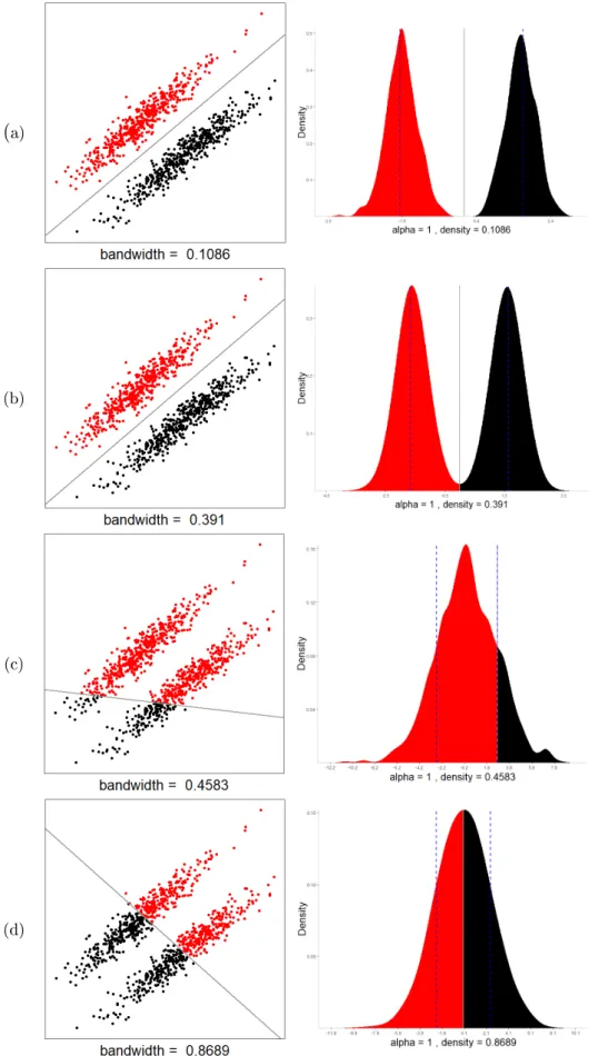
distinct (a-c) and overlapping (d) cluster structures. . . 30 3.4 Eect of kernel bandwidth on MDH solution for distinct cluster
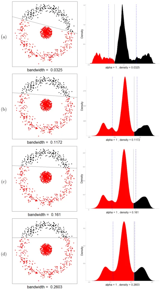
Type A, using: a relatively small bandwidth(a), heuristic band-width (b), full bandband-width (c) and large bandband-width (d). . . 32 3.5 Eect of kernel bandwidth on MDH solution for distinct cluster
Type B, using: a relatively small bandwidth(a), heuristic bandwidth (b), full bandwidth (c) and large bandwidth (d). . . 33 3.6 Illustration of Minimum Density Hyperplane estimation through
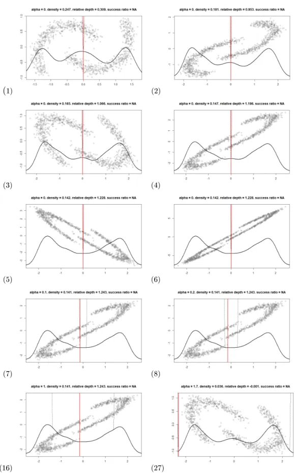
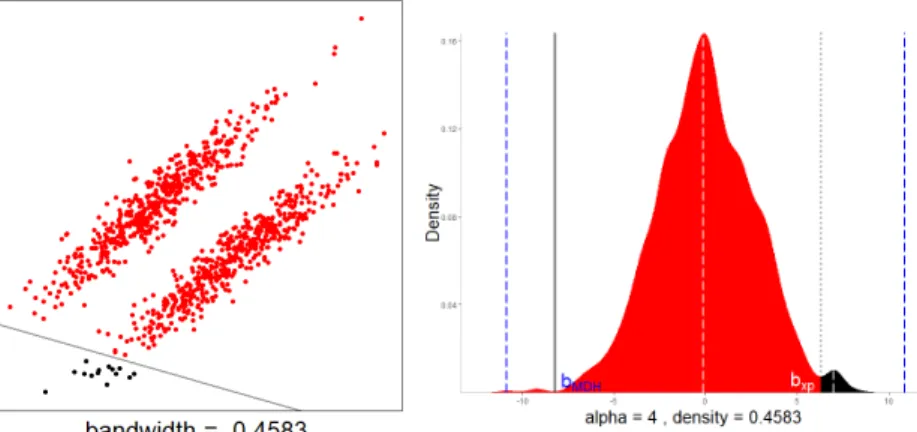
dierent iterations utilising incremental α values. Each gure is accompanied by a number representing the overall iteration within the MDH solution. . . 35 3.7 MDH solution of linearly separable data using a relatively large
bandwidth and setting w= 2. The blue dashed lines represent the
maximum feasible region, scaled be α and the white dashed lines represent the Mw=2 interval . . . 36
4.1 Mean Shift clustering of distinct (a-c) and non-distinct (d) group-ing. Minimum cluster size was set to 245 observations. . . 41 4.2 Mean Shift reassignment of distinct cluster Type B MDH solution
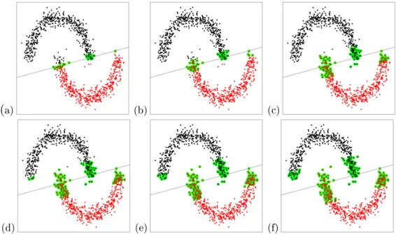
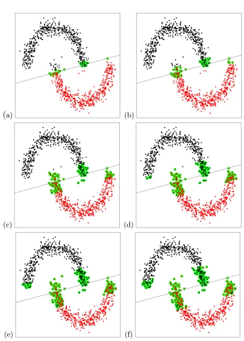
over: Γ0.05 region (a),Γ0.10 region (b),Γ0.20 region (c),Γ0.25 region (d), Γ0.30 region (e),Γ0.35 region (f). . . 42 4.3 Heuristic reassignment of distinct cluster Type B MDH solution
over: Γ0.05 region (a),Γ0.10 region (b),Γ0.20 region (c),Γ0.25 region (d), Γ0.30 region (e) and Γ0.35 region (f). . . 44 4.4 Gradient heuristic Type B solution using Γ0.35. Large blue points
represent the Mean Shift estimated modes, green lines indicate gra-dient ascent trajectories with yellow indicating those which initially move towards the hyperplane but do not converge beyond the hy-perplane. . . 45 4.5 The Banknote data's MDH solution density plots; using the
heuris-tic (a), full (b) and experimental (c) bandwidths. The red, green and black areas represent cluster 1, Gamma region and cluster 2 respectively. . . 49 4.6 The Banknote data's restricted MDH (w = 2) solution density
plots; using the heuristic (a), full (b) and experimental (c) band-widths. The red, green and black areas represent cluster 1, Gamma region and cluster 2 respectively. . . 50 4.7 Boxplots of Success Ratios for standard (w = 0) and restricted
(w= 2) MDH solutions overall (left) and per dataset (right). . . 51
4.8 The change in MDH Success Ratio's across various kernel band-widths per Mean Shift and the single step reassignment procedures. Zero indicates the SR of the original MDH solution. . . 52 4.9 The change in MDH Success Ratio's across various Gamma region
sizes per Mean Shift and the single step reassignment procedures. Zero indicates the SR of the original MDH solution. . . 52 5.1 Image of a red square atop green background (a) with associated
scatter plot of pixels in three dimensions (b) and density estimate ofvvv>X projection with decision boundary at zero indicated by the dashed line (c). . . 55 5.2 Image of the dog (a) with associated scatter plot of pixels in three
dimensions (b), colour matched for clarity. . . 58 5.3 Minimum Density Hyperplane solution (a) and associated scatter
plot of pixels (b), colours represent the average RGB channel in-tensities from clusters assigned by separating plane. . . 58 5.4 Density of the nal univariate projection of the MDH solution (a)
and density resulting from projecting onto the second principal component (b). The hyperplane is the red line and the maximum feasible region is indicated as dashed lines. . . 59
5.5 Solution (c) using density estimate of projection onto the second principal component axis (a) with the manually chosen plane in red and with clusters in RGB space(b). . . 60 5.6 Decorrelated and stretched dog image (a) with associated scatter
plot of pixels (b), colour matched for clarity. . . 61 5.7 Minimum Density Hyperplane solution from decorrelated and stretch
dog image (a) with its associated scatter plot of pixels (b). . . 62 5.8 Density of the nal univariate projection of the MDH solution (a)
and the second principal component projection density (b) from the decorrelated and stretched dog image. The hyperplane is indicated in red, with the feasible region contained within the dashed lines. . 62 5.9 Mean shift adjusted MDH dog image with associated scatter plot of
points around solution plane: Γ0.15 reassignment region indicated by blue coloured points (a), reassigned points indicated in red (b) and nal adjusted solution (c). . . 63 5.10 Heuristic adjusted MDH dog image with associated scatter plot of
points around solution plane: Γ0.15 reassignment region indicated by blue coloured points(a), reassigned points indicated in red(b) and nal adjusted solution(c). . . 64 5.11 Decorrelated and stretched MDH solution mapped to original image
colour space; Γ0.20 region indicated by blue coloured points (a), reassigned values in red (b) and nal solution (c) with associated scatter plots below each image . . . 65 5.12 Binary image segmentation results from 2-means, MMC, MDH,
MDHΓM S and MDHΓH procedures. . . 68
B.1 Mean Shift assignment for Type A and Type C data types with local modes indicated as blue dots. . . 76 B.2 Mean Shift cluster assignment for Type C and Type D datasets. . . 77 B.3 Mean Shift reassignment of distinct cluster Type A with: L= 0.05
(a),L= 0.10(b),L= 0.20(c),L= 0.25(d),L= 0.30(e),L= 0.35
(f). . . 78 B.4 Mean Shift reassignment of distinct cluster Type C with: L= 0.05
(a),L= 0.10(b),L= 0.20(c),L= 0.25(d),L= 0.30(e),L= 0.35
(f). . . 78 B.5 Mean Shift reassignment of distinct cluster Type D with: L= 0.05
(a),L= 0.10(b),L= 0.20(c),L= 0.25(d),L= 0.30(e),L= 0.35
(f). . . 79 B.6 Heuristic reassignment of distinct cluster Type A with: L = 0.05
(a),L= 0.10(b),L= 0.20(c),L= 0.25(d),L= 0.30(e),L= 0.35
(f). . . 79 B.7 Heuristic reassignment of distinct cluster Type C with: L = 0.05
(a),L= 0.10(b),L= 0.20(c),L= 0.25(d),L= 0.30(e),L= 0.35
B.8 Heuristic reassignment of distinct cluster Type D with: L = 0.05
(a),L= 0.10(b),L= 0.20(c),L= 0.25(d),L= 0.30(e),L= 0.35
(f).. . . 80 B.9 Heuristic assignment of distinct cluster Type D. Large blue points
represent the estimated modes from MS, green lines indicated gra-dient ascent trajectories with yellow indicating those paths which move towards but do not converge beyond the hyperplane. . . 81 C.1 Two identied pixels within the dog image with their associated x,
y and RGB values. . . 83 C.2 Subset of dog image highlighting brown tones within the image (a)
and the associated scatter plot of pixels (b). . . 84 C.3 Pixel intensities for non-transformed (a) and decorrelated stretched
(b) dog image. . . 84 C.4 Binary cluster results of Dog Image (a) using 2-means (b), Max
Margin Clustering (c), Minimum Density Hyperplane Clustering (d), MDH solution reassigned by Mean Shift (e) and the single step gradient procedure (f). . . 85
List of Tables
4.1 Comparison of MDH and MS solutions. . . 41
4.2 Details of benchmark datasets. . . 46
4.3 Benchmark datasets' Success Ratios using w= 0 and h. . . 47
4.4 Benchmark datasets' Success Ratios using w= 0 and h∗. . . 47
4.5 Benchmark datasets' Success Ratios using w= 0 and hxp. . . 47
4.6 Benchmark datasets' Success Ratios using w= 2 and h. . . 48
4.7 Benchmark datasets' Success Ratios using w= 2 and h∗. . . 48
4.8 Benchmark datasets' Success Ratios using w= 2 and hxp. . . 48
5.1 Subset of image segmentation results from comparative study . . . 69
A.1 Euclidean distance dissimilarity matrix. . . 75
B.1 Class details of benchmark datasets. . . 82
Chapter 1
Clustering for Image Segmentation
1.1 Introduction
Image segmentation is a eld within computer vision that attempts to auto-matically segment objects in a picture similar to how the human visual system does (Ballard and Brown, 1982). Image segmentation most often forms the initial step for object detection or pattern recognition. An image is represented as a collection of pixels, each containing a measurement of colour or light inten-sity. There are two common types of images, grayscale and colour. Frequently an image will exhibit a foreground which contains pixels that are more similar to one another than to those contained in the background. Grouping pixels which are similar, provides a logical approach to segmenting an image. Several cluster analysis techniques have been presented as possible solutions for image segmentation.
Cluster analysis is an unsupervised approach that attempts to learn the true underlying class structure within a dataset (Tan et al., 2013). When considering image segmentation, cluster analysis seeks to learn the relational structure of pixel intensities in order to detect patterns within an image. While the human visual system can easily identify objects within an image, the task is notably more dicult for computers. The ability for an application to cluster objects in an automatic way is an important data mining tool which serves as a solution for image segmentation.
There is a plethora of clustering techniques available to analysts. Each technique provides a dierent approach to grouping and is accompanied with its own set of challenges. The challenges for any given method can be sum-marised by its constraints, scalability, quality and usability (Tan et al., 2013). The more popular methods embody few constraints, scale well and produce meaningful, useful clusters.
Density-based clustering methods are a popular choice for attempting to solve the task of image segmentation. These techniques are capable of learn-ing complex structures within a dataset. However, most density-based
ods suer from a lack of scalability. Minimum Density Hyperplane (MDH) clustering is a recent procedure that scales relatively well compared to other density-based approaches. MDH attempts to solve the problem of learning an optimal low-density linear separator via projecting onto a univariate vector. This achieves maximal reduction in dimensionality and results in MDH being more applicable to larger scale problems than other density-based methods. MDH learns an equation which denes the hyperplane solution which allows for deriving solutions from a subset of the data. Other popular density-based methods, such as the well known spatial clustering of applications with noise (Ester et al., 1996, DBSCAN), require a full dataset to obtain a solution and are incapable of sampling to reduce computation. Herein lie some key ad-vantages that MDH has over most other density-based clustering techniques, scalability and its ability to cluster a full dataset using only a subset of the data.
One limiting factor associated with an MDH solution is that the nal group-ings are determined using a linear hyperplane. Thus, MDH is not able to learn the true underlying class structure of data containing clusters which are not linearly separable. Yates and Pavlidis (2016) presented a method which non-linearly embeds data into a high-dimensional feature space using Kernel Principal Component Analysis (Schölkopf et al., 1998, KPCA). MDH is then applied to the embedded data. The linear separator in the feature space then corresponds to a non-linear surface in the input space. This method has been shown to be eective but can be computationally expensive with a complex-ity of O(n2), where n is the number of observations. This thesis provides a dierent approach to improving the hyperplane solution, whereby objects in a neighbourhood around the decision boundary are reassigned using gradient ascent. Applying gradient ascent to a region around the low-density separa-tor allows for a nal solution which is not constrained by a linear decision boundary and therefore may improve the hyperplane solution.
Mean Shift (Cheng, 1995, MS) is a gradient ascent approach that assigns objects to clusters based on their location within an attraction basin according to an estimated mode of the probability density function underlying the data. Mean Shift has the same time complexity as KPCA, O(n2), but since we only
consider a subset of the data, the complexity is greatly reduced. Frequently, the gradient ascent trajectory of an observation will not change direction in relation to the hyperplane. We present a heuristic approach to MS based on the initial gradient which further reduces the computation involved with reas-signing observations. This procedure calculates the gradient of the probability density function evaluated at a point and reassigns the observation based on the initial gradient in relationship to the hyperplane. If the estimated gradient points towards the hyperplane then it is likely that the gradient ascent trajec-tory will have converged to a mode opposite the hyperplane and thus signals that the observation should be reassigned to a dierent cluster.
1.2 Outline
The research undertaken in this thesis is aimed at enhancing the Minimum Density Hyperplane solution by applying a gradient ascent procedure, in the style of MS, to a set of points within a predened distance to a hyperplane solution. A single step gradient heuristic approach is also evaluated as an attempt to reduce the computational expense involved with MS.
The remainder of this thesis is organised as follows: Chapter 2 outlines cluster analysis, presents a brief survey of clustering techniques, describes a few methods that measure the quality of a clustering solution before conclud-ing with a discussion about various real-world applications. Chapter 3 details Minimum Density Hyperplane clustering and introduces a novel constraint to the location of a hyperplane solution. Chapter 4 describes two methods to improve the hyperplane solution, namely Mean Shift and its heuristic counter-part. These enhancements are evaluated across several benchmark datasets. Chapter 5 illustrates MDH as an image segmentation tool and discusses a pre-processing method that disperses pixels, which can assist with locating an optimal low-density separator. Then an image segmentation comparative study is undertaken using a variety of images, comparing the performance between K-means, Maximum Margin Clustering, MDH and its enhancements. Chapter 6 concludes the thesis with a discussion on the scope and limitations of the proposed enhancements and proposes future research regarding enhancing hyperplane solutions.
Chapter 2
Cluster Analysis
2.1 Introduction
Cluster analysis is an important data mining tool for exploring and under-standing information contained within a dataset (Kassambara, 2017). The term cluster analysis (or clustering, data segmentation) refers to a broad set of statistical methods which partition objects into groups which have similar characteristics (James et al., 2013). Clustering is known as an unsupervised machine learning method, since it groups observations within a dataset by learning the composition of clusters without any prior knowledge. Each object can be dened by either a set of measurements or by its relationship to other objects. One common objective of clustering is to divide observations into homogeneous and distinct groups, such that objects within a cluster are more similar to one another than those assigned to other clusters (Hartigan, 1975). There are two fundamental concepts that dene the goals of cluster analysis; the notion of similar and the meaning of distinct groups.
The notion of dissimilarity/similarity is central to determining how ob-servations are grouped within cluster analysis. Similarity is dened as how similar one element is to another and conversely, dissimilarity is dened as how dierent an element is to another. Often, clustering is based on pairwise dissimilarity measures between objects. One common metric used to dene dis-similarity is Euclidean distance (special case of Minkowski distance, L2norm). Consider a simple example of persons' height and weight (Figure 2.1). As with most 2-dimensional graphical representations, points are represented as a pair of numerical coordinates (x, y), in accordance with the Cartesian co-ordinate system. Euclidean distances are measurements between points along the Cartesian plane (Equation A.1.1). Since Euclidean distances are dened along the Cartesian plane, it is possible to infer similarities and dene clusters by viewing a scatter plot of the data, given the data consists of three or fewer dimensions and the axis measurements are of equal ratio. The ratio of the axis is important since cluster analysis is not scale invariant with respect to
changes of units in a single axis. One should bear this in mind before applying a method that utilises Euclidean distances and consider whether measurements require scaling (Edwards and Cavalli-Sforza, 1965). From the simple example of persons' height and weight, two distinct clusters are evident, one cluster contains subjects a and e while the other group consist of b, c and d.
Subject Weight Height
a 65 140
b 120 180
c 110 175
d 110 195
e 68 152
Figure 2.1: Simple example of persons' height and weight.
The choice of distance measure is important since clusters formed by one dissimilarity measurement can be very dierent than those derived from oth-ers. When possible, the choice of dissimilarity metric should be based on pre-existing knowledge of the data (Friedman et al., 2001). As an alternative to grouping observations based on distance metrics, one could dene clusters using densities. Density-based techniques dene clusters as a group of obser-vations sharing a common estimated probability density mode. Density-based clustering is central to this text and is more aptly detailed in Section 2.3.4. The various dissimilarity/similarity metrics will not be covered in this text and interested readers are referred to Cox and Cox (2000). Attention now turns to the meaning of distinct groups.
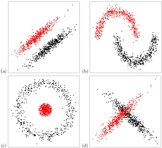
Carmichael and Julius (1968) dened distinct groups as contiguous, densely populated areas within a dataset which are separated by contiguous relatively empty regions. Figure 2.2 illustrates some examples of distinct groups (a-c) and one which is considered indistinct (d), according to the denition by Carmichael and Julius (1968). For the remainder of this thesis, these distinct data structures are referred to as;T ype Afor linearly separable (Figure 2.2(a)), T ype B for non-linearly separable (Figure 2.2(b)),T ype C for dynamically sep-arable (Figure 2.2(c)) andT ype D refers to overlapping classes (Figure 2.2(d)). While many algorithms seek to divide the data into distinct groups, there are
techniques which allow for overlapping cluster solutions, such as fuzzy clus-tering. For the purpose of this text, these techniques will not be covered and interested readers are directed to Evers et al. (1999) for further details on fuzzy-based clustering methods.
(a) (b)
(c) (d)
Figure 2.2: Linearly separable (a), non-linearly separable (b), dynamically sep-arable (c) and overlapping group (d) dataset structures.
Cluster analysis is utilised extensively within data mining. It serves two main utilities: it can be used as a pre-processing utility for application in other algorithms and/or as a stand-alone tool to derive insight into the distribution of a dataset. Cluster analysis has rich applications across multiple research disciplines. The goal of this chapter will be to elaborate on these statements while providing general insight into various clustering techniques. The remain-der of this chapter is organised as follows: We begin by reviewing the two main purposes of clustering. This is followed by a brief survey of clustering tech-niques. Afterwards the topic of cluster validation and assessment is discussed. Lastly, a few practical applications in key research disciplines are discussed before concluding the chapter with a summary.
2.2 Main Purposes
Cluster analysis can be summarised as serving one of two typical purposes; stand-alone or an intermediate tool. As an intermediate tool, clustering can be used as a pre-processing step for other algorithms. As a stand-alone tool, cluster analysis is utilised to gain insight into the underlying structure present within data. We begin with a discussion on how cluster analysis can be utilised as an intermediate tool.
2.2.1 Intermediate tool
Clustering is useful as an intermediate step for other data mining tasks such as generating a compact summary of data for classication, hypothesis testing and outlier detection (Tan et al., 2013). Cluster analysis can be utilised as a preprocessing step for other algorithms to reduce computational expense. This section focuses on ways in which cluster analysis can be used as a data reduction technique.
In cluster analysis a group can be characterised according to a cluster prototype or prototypes. A prototype is an object or position within a cluster that is an ideal representation of all other observations within the cluster (Tan et al., 2013). These prototypes are often represented by the mean or medoid of all points within a cluster. The mean is typically used when observations are continuous while the mediod is ideal for discrete categorical data or when the mean cannot be dened. A medoid prototype is an element within a cluster which exhibits the lowest average distance to all other objects within its group (Struyf et al., 1997). Dening the most representative cluster prototypes is useful for multidimensional scaling and as a method to eciently nd nearest neighbours (Friedman et al., 2001).
If a given number of cluster prototypes represent the overall data structure well, then these prototypes can be used as inputs for data modelling. Well positioned prototypes can produce similar results to what the full dataset would have produced (Tan et al., 2013). Utilising a set of cluster prototypes, of size smaller than n, reduces the space and time complexity required by a statistical procedure. For instance, in nearest neighbour applications the pairwise distance between all points is required. Using well positioned cluster prototypes in place of points, reduces the number of distance calculations required. Thus, locating the nearest neighbour prototype for any given object only requires computation of the distance from said object to all prototypes (Friedman et al., 2001).
Clustering provides a meaningful method for dimension reduction when data contain a large number of covariates (d). Gene expression data often contain more covariates than observations, i.e. d > n (Eisen et al., 1998). In this case, multiple linear regression using least squares is not possible since
the number of coecient estimates exceeds the number of observations (James et al., 2013). Utilising clustering as a dimension reduction technique to reduce the number of covariates by representing them as cluster prototypes (d∗, with d∗ < n) allows for the application of statistical methods which would otherwise not be possible.
2.2.2 Stand-alone tool
In today's big data world, clustering is a valuable stand-alone tool. Clustering plays an important role in online recommendation systems for Amazon, Netix, and YouTube (Linden et al., 2003). Essentially, cluster analysis seeks like-minded users in order to provide services which will most likely cater to their desires.
Clustering can also provide a framework for a new classication structure. In order to understand a new object or phenomenon, researchers explore the dataset dening said object and compare it with closely related known objects using cluster analysis (Xu and Wunsch, 2005). The hope is that identify-ing these clusters will increases the overall knowledge and understandidentify-ing that people will have of this phenomenon in the future. This automatic learning process plays an important role in several elds of research. These include but are not limited to: biology, medicine, psychiatry, economics and multimedia analysis. The role that clustering serves within said elds is further discussed within Section 2.5.
Clustering is also a common tool for spatial data analysis (Halkidi et al., 2001a). Spatial data consist of information that identies various objects such as oceans, naturally occurring and constructed features, commercial and residential zones and socio-economic indicators to name a few (Bailey and Gatrell, 1995). Given the size of such datasets, it is labour intensive and most often infeasible for analysts to manually examine spatial data in detail. Clustering provides an automatic process for analysing data by identifying and extracting useful patterns and characteristics that may exist (Halkidi et al., 2001a).
Clustering as a stand-alone application is also popular within computer vision, utilised as a multimedia processing and query technique. In this re-gard, clustering can be utilised to identify interesting shapes within images, track objects within videos, compress multimedia les to reduce storage re-quirements and provide a system for fast retrieval of information contained online (Berkhin, 2006). Image segmentation is the process which partitions an image into dierent segments which contain similar attributes (viz. pixel intensities). It can be considered a pre-processing step also if one is concerned with object recognition, tracking or image analysis (Kumar, 2017). One can segment a single image and then group a collection of segmented images based on similarities which can then decrease the required time to query such in-formation. These systems are popular for online image queries, such as that
utilised within Google's image search engine (Deselaers et al., 2003). Image segmentation using clustering is the topic of Chapter 5. Therein, image seg-mentation is discussed and illustrated in further detail with an emphasis on enhancing density-based hyperplane solutions.
2.3 Clustering Methods
There is a plethora of clustering methods available to analysts. Each tech-nique may provide dierent groupings and is accompanied with its own set of challenges. The choice of a particular algorithm is dependent on: desired out-put, known ability of the method to learn various cluster structures, and the type and size of the dataset in question (Berkhin, 2006). There are two broad classes of clustering, hierarchical and partitioning. Hierarchical techniques sequentially merge observations into clusters (agglomerative algorithms) or divide a dataset into smaller clusters (divisive algorithms). Partitioning meth-ods segment a dataset of n objects into k mutually exclusive clusters. The key dierence between partitioning and hierarchical procedures is that hier-archical methods build clusters iteratively while partitioning techniques learn groupings directly.
Clustering methods can be further categorised into ve broad kingdoms: partitioning, hierarchical, model-based, density-based and grid-based methods (Tan et al., 2013). Some algorithms contain a mixture of these categories and as such some methods can reside within multiple kingdoms. Nevertheless, this scheme of grouping methods is common and assists with discussing attributes of the various clustering techniques.
The challenges for any given method can be summarised by its constraints, scalability, quality, interpretability/usability. The constraints of a technique refers to user-specications that are required in order to apply a given clus-tering method. Scalability indicates the eciency of a technique to obtain a clustering solution from large datasets. The quality of a method is predicated upon its ability to deal with dierent data types, discover clusters of complex shape and if it is capable of dealing with outliers or noisy data. Interpretability of a clustering technique is dened as whether the method produces meaning-ful clusters which describes the data well and can be easily understood and used by many people (Aggarwal and Reddy, 2013). The following subsections briey discuss the various clustering methods and the challenges accompanying each technique.
2.3.1 Partitioning methods
Partitioning methods segment n objects into k groups which optimise a cho-sen partitioning criterion. There are methods which exhaustively enumerate all partitions seeking the optimal solution and those which apply a heuristic
approach, such as K-means. A common constraint of partitioning methods is that they require the user to pre-dene the number of clusters (Xu and Wun-sch, 2005). K-means is one of the most popular partitioning-based clustering techniques.
K-means is a technique intended for data which is quantitative where dis-similarities are dened using Euclidean distance and the objective is to min-imise within and maxmin-imise between cluster variability. The standard K-means algorithm was rst presented by Stuart Lloyd in 1957 while working at Bell Labs, which was later published in 1982 (Lloyd, 1982). James MacQueen et al. (1967) was the rst to coin the term, "K-means". The main concept is to dene k centroids, one for each cluster. The procedure begins by randomly/manually selecting k points within the input space of interest. These points represent the initial cluster centroids or prototypes. Then, each observation is assigned to its nearest prototype. Once all objects are assigned to a cluster, a new pro-totype is calculated for each group. This process repeats until no observations move from one cluster to another.
K-means is well known since it is relatively straightforward and based on the foundation of analysis of variances. An upside to K-means is that it can be an ecient method. The most popular K-means algorithms requireO(tkn) calculations, where t represents the number of iterations, k is the number of clusters and n represents the sample size. These algorithms scale well since normally the number of clusters and iterations required to obtain a cluster-ing is far fewer than the number of observations (Hartigan and Wong, 1979). However, results from K-means strongly depend on the initial points and each solution is based on local optima which tends to be far from the global one (Berkhin, 2006). Furthermore, in some instances empty clusters may be formed from K-means due to poor initialisation. As with all partitioning methods, it is often not obvious what a reasonable value of k should be. Also, outliers can inuence cluster structures when the squared error criterion is used (Tan et al., 2013). K-means cannot discover clusters with non-convex shapes and is applicable only when a dataset is continuous Hartigan (1975).
There are several adaptations of K-means to work around the various short-comings. K-means++, introduced by Arthur and Vassilvitskii (2007) sought to solve the problem of initialisation points. K-modes reduced the impact of noisy data while having the ability to handle categorical data (Huang, 1997). Kernel K-means are partitioning methods brought forth to handle non-convex cluster structures (Dhillon et al., 2004).
The constraint of selecting the number of clusters is a common deterrent for partitioning methods. As with all clustering techniques, the choice of par-titioning method will impact scalability, quality and the interpretability of the nal results.
2.3.2 Hierarchical methods
Hierarchical clustering methods derive groups through a nested sequence of dividing or combining observations into clusters based on an optimisation cri-terion and notion of similarity (density or distance-based). Cluster structures derived from hierarchical methods can be represented by dendrograms, hence the name hierarchical clustering. One strength of hierarchical methods is that they do not require a pre-dened number of clusters. One limitation is that iterative renement cannot be applied to previously constructed clusters (Wu et al., 2008).
There are two main approaches to hierarchical clustering, top-down (di-visive) or bottom-up (agglomerative). Divisive algorithms are considered a global approach whereby the initial cluster contains all observations within the dataset, which is then recursively divided into smaller groups until each object is represented by its own group (singleton). Agglomerative algorithms begin with n singleton clusters and then sequentially join two clusters at a time until all objects are represented by one group (Rousseeuw and Kaufman, 1990).
For divisive methods, the user must pre-dene a splitting criterion. A common splitting criterion, when using Euclidean distances with quantitative data, is Ward's criterion since it seeks a split which produces the greatest reduction in the sums of squared error (Ward Jr, 1963). The Gini-index is a common criterion when the data contain categorical variables (Fisher, 1995).
For agglomerative methods, criteria for joining objects into clusters are pre-dened by the user. The choice of criterion is based on the dissimilarity metric within the algorithm, some common types are: single link (nearest neighbour), complete link (diameter), average link (group average) and centroid link (cen-troid/mean similarity). Each approach denes similarity between clusters dif-ferently. Single linkage denes inter-cluster similarity by the pairwise mini-mum distances between objects from two dierent groups. Complete linkage and average linkage are similar to single linkage but instead consider maxi-mum distances and average distances. Centroid linkage uses prototype mean distances between clusters to dene inter-cluster similarity and combines two clusters that have the smallest centroid distance (Wilks, 2011).
In addition to choosing a splitting or joining criterion, one should specify the number of desired clusters, post hoc. It is obviously not ideal for a cluster to contain only one observation nor the entire dataset. Thus, any desired num-ber of clusters can be obtained by trimming the dendrogram to a meaningful number of groups (Tan et al., 2013). In general, hierarchical methods do not scale well to larger datasets and require at least O(n2) computations, where
n is the number of observations within a dataset. Since hierarchical methods construct clusters in a nested sequence, previous splits and additions cannot be undone. Additionally, it is not always clear which distance metric to apply nor the optimisation criterion to utilise.
Some common hierarchical clustering algorithms which seek to overcome the various shortcomings are: balanced iterative reducing and clustering us-ing hierarchies (BIRCH, Zhang et al. (1996)), clusterus-ing usus-ing representa-tives (CURE, Guha et al. (1998)) and hierarchical clustering using dynamic modeling (CHAMELEON, Karypis et al. (1999)). Each of these methods at-tempt to solve the various challenges posed by hierarchical clustering. CURE is robust to outliers, BIRCH scales linearly which reduces complexity and CHAMELEON can learn complex cluster structures within datasets.
2.3.3 Model-based methods
Model-based methods are a more formal, parametric approach to solving the clustering problem. These methods assume that each cluster is represented by a density which is assumed to be a member of some parametric family, such as Gaussian or Poisson distributions. Consider that X = {xi}ni=1 denes a dataset consisting ofni.i.d. observations ind-dimensions with joint probability density p(x). The goal is to identify the underlying probabilistic properties of
this joint density so as to infer relational structures within the data (Friedman et al., 2001). Model-based methods use a pre-specied mixture of densities, based on what is believed to represent the cluster structure within a dataset. These densities combine to represent the overall underlying probability density function. Then each component's associated parameters are estimated and used to cluster observations based on a pre-dened criterion, such as Bayes' rule (Fraley and Raftery, 1998).
Model-based approaches require k parametric distribution assumptions. The choice of an optimal number of clusters is attenuated by applying paramet-ric tests such as the Bayesian or Akaike information criterion across multiple choices ofk(Fraley and Raftery, 1998). Model-based approaches are exible in the sense that one can choose the distributional composition. These methods are easily understood since they are based upon statistical theory. Model-based approaches can handle missing data and directly model the density of each cluster (Kumar, 2017).
2.3.4 Density-based methods
Density-based methods are the non-parametric alternative to model-based techniques. Clusters are dened as areas of high density separated by regions of low densities. Densities are estimated from a dataset X⊂Rdconsisting of the realisations of a random variable with an underlying unknown probability den-sity functionp(x). The subsequent clusters can be dened in one of two ways;
as a set of maximally connected components of level sets {x ∈ Rd|p(x) > λ} based on a sensible choice for the level parameter λ (Hartigan, 1975; Rinaldo and Wasserman, 2010) or as a group of observations within the same attraction basin dictated by a probability density function (Azzalini and Menardi, 2014).
An attraction basin is dened as the region for which all observations' gradi-ent ascgradi-ent trajectories lead to the same estimated mode. Modal regions are dened herein as the area consisting of all observations within an attraction basin sharing a common mode. The benet of most density-based methods is that a user does not need to pre-specify the number of clusters, such as the case with DBSCAN and Mean Shift clustering (Ester et al., 1996; Cheng, 1995).
DBSCAN is a well known method proposed by Ester et al. (1996). A ben-et from DBSCAN is that it can identify complex cluster structures within noisy datasets. This technique is robust to outliers as it incorporates a no-tion of noise, whereby removing points which are considered outliers. Users do not need to specify the number of clusters but must dene the minimum amount of observations required for each group, and an-neighbourhood value. The-neighbourhood value dictates the window, bandwidth or distance radius around a point to consider when clustering (Ester et al., 1996). One shortcom-ing of DSCAN is that it does not scale well, with a time complexity of O(n2). However, this can be reduced toO(nlog(n)) by using ecient structures found
in lower dimensional spaces of the data (Hinneburg et al., 1998).
Mean Shift (Cheng, 1995, MS) is a mode-seeking procedure that utilises gradient ascent based on Gaussian kernels to assign clusters within a dataset. MS is commonly utilised as a stand-alone method for image segmentation, vi-sual tracking, space analysis and mode-seeking (Fukunaga and Hostetler, 1975; Comaniciu and Meer, 1999; Comaniciu et al., 2000). Mean Shift does not as-sume any prior cluster structure. It can learn non-convex clusters and is robust to outliers. The only requirement is that a user must specify the window size. The choice of window size (Parzen window or kernel bandwidth) represents a trade-o between generality and accuracy. Selecting a window size is not trival and ultimately determines the nal output. Larger values increase the overall smoothness of an estimated probability density and can cause modes to merge. Conversely, smaller values decrease smoothness and generate additional shal-low modes. To mitigate the problem of bandwidth selection, one can use an adaptive window size (Comaniciu et al., 2001). MS has a time complexity of O(n2) and does not scale well to larger datasets. However, complexity can be reduced to O(nlogn) if only neighbouring observations are considered during the computation of MS (Cheng, 1995).
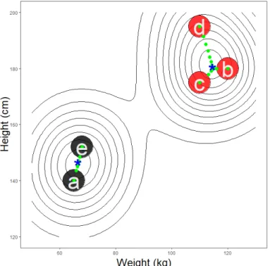
Consider again the example of person's height and weight. Figure 2.3 illustrates how MS clusters the data. The contour lines represent the estimated probability density function. These contours provide a visualisation of the attraction basins. Person d is within the attraction basin dictated by the right-most mode and as such is assigned to the cluster containing persons b, c and d. Each object's gradient ascent trajectory is indicated as green dots. Notice that each object requires a dierent number of iterations to converge to a mode. Points further away require more iterations than those closer to their respective mode. Data structures with greater variance may require relatively
more iterations than those containing less variability. MS is discussed in more detail in Chapter 4.
Figure 2.3: Mean Shift solution path from clustering the simple example of persons' height and weight. Green points represent the gradient ascent path of each element towards its associated mode (blue asterisks).
Minimum Density Hyperplane (Pavlidis et al., 2016, MDH) clustering is a recent technique which scales relatively well compared to other density-based methods, such as MS and DBSCAN. MDH clusters observations by directly identifying a low-density separator that partitions at least one dense region from all others, using projection pursuit. The integral of the empirical density function along a hyperplane which is a minimiser represents the low-density separator according to the formulation posed by Ben-David et al. (2009). Pro-jection pursuit seeks the linear transformation that results in a highly separa-ble space, whereby the integral of the probability density function along the hyperplane is minimised. Maximal dimension reduction is achieved by pro-jecting onto a vector. This is particularly advantageous for high-dimensional problems. Since MDH yields a binary partition, it cannot learn more than two clusters from a dataset. Minimum Density Divisive Clustering (Hofmeyr and Pavlidis, 2018, MDDC) is an extension of MDH which is capable of cluster-ing more than two groups by creatcluster-ing a hierarchical collection of hyperplanes. Also, since MDH denes clusters using a hyperplane, it is incapable of learning cluster structures which are not linearly separable. In this thesis we formulate
a technique to overcome this limitation by applying a gradient ascent proce-dure to a collection of observations around the hyperplane solution. MDH is discussed in further detail in Chapter 3 and the proposed enhancement to the hyperplane solution are detailed in Chapter 4.
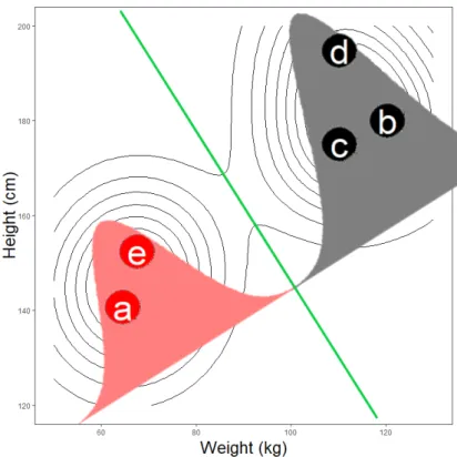
Figure 2.4 illustrates how MDH assigns the simple example of person's height and weight to clusters, using a univariate estimated density function along the direction orthogonal to the minimum density hyperplane, which is indicated as a green line. Observations that lie below the hyperplane solution are assigned to the red cluster (a and e). Conversely, those above the plane are assigned to the black cluster (b, c, and d).
Figure 2.4: MDH solution of the simple example of persons' height and weight. The area under the density is coloured to match each assigned cluster and the low-density separator is indicated as a green line.
2.3.5 Grid-based methods
Grid-based clustering is commonly used for data query operations. These methods divide a dataset into a nite number of cells that form a grid structure. Clustering techniques are then applied to the cells within the grid structure. These methods are scalable since typically the number of cells is far fewer than the number of data points. One setback to using grid structures is the diculty in capturing irregular cluster structures within the data across cells.
Also, these methods may suer from local optima due to user-dened cell sizes, borders and density thresholds. Thus, the choice of cell structures crucially impacts nal results. Also, grid-based methods generally perform poorly given high dimensional data (Aggarwal and Reddy, 2013).
One popular grid-based method is known as statistical information grid approach, STING (Wang et al., 1997). STING splits the input space into grids in a divisive hierarchical way, where the rst layer contains few cells and subsequent layers have an increasing number of cells. Parameters dening observations within each cluster are then stored within each cell and used to answer queries. Parameters at higher levels are easily determined by the information contained within its nested levels. STING is an ecient algorithm withO(c) complexity since only relevant cells (c) are recursively explored when processing a query (Wang et al., 1997). Another popular grid-based method is known as clustering in quest, CLIQUE. Interested readers are directed to Agrawal et al. (1998) for further details.
2.4 Cluster Validation And Assessment
Cluster validation and assessment are as diverse as the topic of clustering. Thus, there exist many forms to assess a clustering method. There are three main tasks which cluster validation seeks to address; tendency, stability and assessment. As an initial step, one should evaluate whether a dataset has any underlying cluster structure and if it is even suitable to apply clustering to the data in the rst place. This is known as cluster tendency. Cluster stability evaluates how sensitive a clustering method is to a given set of parameters. Cluster assessment attempts to measure the quality of a clustering solution. Given the multitude of dierent cluster denitions, there is no common method to assess all clustering solutions. In some instances, cluster validation is sub-jective to the user, such is often the case when evaluating image segmentation results. Nevertheless, there are three broad categories for measuring the qual-ity of a clustering algorithm; external, internal and relative measures (Zaki et al., 2014). The following section presents the notation used in the remain-der of this chapter. This is followed by outlining cluster stability, tendency and a discussion of various cluster validation measurements.
2.4.1 Notation
For clarity moving forward, consider that X = {xi}ni=1 denes a dataset in
d-dimensions consisting of n observations partitioned into k classes. Further-more, letyi ∈ {1,2, ..., k}signify the true cluster labels (ground truth) for each point. Let the ground truth partitions be dened asT ={T1, T2, ..., Tk}, where the cluster Tj encapsulates all points with label j, thusTj ={xi ∈X|yi =j}. Clusters dened by a given method will be denoted, C ={C1, C2, ..., Cr} with
ˆ
yi ∈ {1,2, ..., r} representing the assigned labels ofxi. When discussing exter-nal measures, these metrics rely on an r×k contingency table (N) formed by comparing a clustering (C) with the ground truth (T) dened as:
N(i, j) =nij =|Ci∩Tj|, (2.4.1) where nij denotes the common number of objects between the cluster Ci and the ground truthTj. The computational complexity of generating results from this contingency table is O(n), since evaluating each pair, yˆi and yi, from xi ∈Xcorresponds to incrementally adjusting the countnij (Zaki et al., 2014). Furthermore, take notice that the number of true clusters, k, is distinguished from that which is produced by a clustering algorithm, r.
2.4.2 Cluster tendency and stability
Cluster tendency assesses whether the data has any inherent grouping struc-ture. It is dicult to assess given the various ways in which each clustering method denes a cluster. Nevertheless, a few common assessment techniques are spatial histograms, distance distribution and the Hopkins statistic Zaki et al. (2014); Halkidi et al. (2001b).
Cluster stability relies on the premise that clusters obtained from several bootstrapped datasets should be similar or stable. It is typically utilised to determine the optimal number of clusters. The approach begins by taking B bootstrap samples fromXof sizen with replacement. For each ofB bootstrap samples, apply the clustering method for every r value. Then the distances between all pairs of clustering Cr(Xi) and Cr(Xj) are computed to estimate the expected pairwise distance for each value of r. Ultimately, the value of r that exhibits the least amount of variation between the bootstrapped clusters is chosen, as it represents the most stable choice (Zaki et al., 2014).
When considering stability in the context of low-density hyperplanes, there exists a signicant relationship. Essentially, a hyperplane solution associated with a lower integrated density is considered more stable than those with rel-atively higher associated integrated densities (Ben-David and Von Luxburg, 2008). Those hyperplane solutions which are associated with relatively larger integrated densities tend to yield highly variable solutions compared to hyper-plane solutions with lower densities.
2.4.3 External measures
External cluster validation compares a clustering solution C against an ex-ternally provided set of ground truth labels, T. External measures are su-pervised validation techniques that require some prior knowledge of the class structure within a dataset. External measures are utilised to gain insight into
how well a given algorithm recovers the known class structure (Kassambara, 2017). Quality clustering methods are considered as those which produce pure, homogeneous clusters which assign observations to their true class, clus-ter completeness. Additionally, to include a heclus-terogeneous element into a pure cluster should be penalised more than if it was clustered into a miscellaneous or less homogeneous category. Also, dividing a relatively smaller sized cluster into further segments is considered more harmful than splitting a cluster con-taining a relatively greater number of observations (Zaki et al., 2014). Some commonly used external validation metrics include: matching-based, entropy-based, pairwise and correlation measures. A more recent external measure known as Success Ratio was proposed by Pavlidis et al. (2016), which captures the binary partition performance of a given clustering method.
2.4.3.1 Success Ratio
The Success Ratio is a metric which expresses how well a clustering algorithm groups data into two clusters. While this method is ideal for two-class datasets, it can be extended to data containing more than two classes. In such scenarios, when k is greater than two, labels are aggregated by assigning each element to the group which contains the majority of its members. The Success Ratio indicates how distinct the majority of at least one cluster is from the rest of the data. Success ratio values of zero indicate that an algorithm failed to locate the majority of any cluster from within the data. Larger values signal a better quality of clustering. Values of one indicate that all clusters remain intact after the binary partition. Thus, a good binary partitioning method is one that clusters at least one class to a group that is distinct from all others within the data (Pavlidis et al., 2016).
To calculate the Success Ratio when k is greater than 2, the true class labels are aggregated, denoted T∗
1 and T ∗
2. Then, the binary partition error
E(C1,C2) is calculated as dened in Equation 2.4.1. Essentially, the binary partition error represents the number of objects which are not grouped with the cluster containing the majority of its true class members. In contrast, the success of a cluster, S(C1,C2), captures the extent to which observations are grouped to a cluster containing the majority of their original class mem-bers (Equation 2.4.2). Overall, the Success Ratio (SR(C1,C2)) measures the capability of a clustering technique to cluster the data such that it does not separate observations belonging to the same class (Pavlidis et al., 2016). The Success Ratio is dened as:
E(C1,C2) =min n |C1∩ T1∗|+|C2∩ T2∗|,|C1∩ T2∗|+|C2∩ T1∗| o (2.4.2) S(C1,C2) =minnmax |C1∩ T1∗|,|C1∗∩ T2∗| , max |C2∩ T1∗|,|C2∩ T2∗| o (2.4.3) SR(C1,C2) = S(C1,C2) S(C1,C2) +E(C1,C2) (2.4.4)
2.4.4 Internal measures
Internal measures are unsupervised methods which assess the quality of a clus-tering method based solely on the data. Internal metrics attempt to capture the extent of how similar objects are within clusters (cluster compactness) and the dissimilarity between clusters (separation). Intra-cluster compactness and inter-cluster separation are obtained via pairwise distance measurements dened by δ(xi,xj), which is assumed to be the Euclidean distance between xi,xj ∈X(Zaki et al., 2014). When possible, the choice of dissimilarity matrix used to calculate the quality of clustering should coincide with that used to dene the clusters. Overall, internal metrics produce a trade-o between max-imising intra-cluster compactness and inter-cluster separation (Halkidi et al., 2001b; Zaki et al., 2014).
These metrics are motivated by dening a good clustering algorithm as one which produces groupings with high intra-class similarity and high inter-class dissimilarity. One commonly used internal cluster validation measure is the silhouette coecient (Kassambara, 2017).
2.4.4.1 Silhouette coecient
The silhouette coecient measures how similar objects are within a cluster and the separation between groups. It captures this as a ratio of how close a point is to all other objects within its cluster and how far it is to those points in a neighbouring cluster. The overall silhouette coecient is the average of each observation's coecient si which is calculated as:
si= µminout (xi)−µin(xi) max µmin out (xi), µin(xi) , (2.4.5)
where µin(xi) represents the mean distance between xi and all other observa-tions within its cluster Cˆyi and dened as:
µin(xi) = P xj∈Cyiˆ,j6=iδ xi,xj nyˆi−1 , (2.4.6)
and µminout (xi) represents the mean distances between xi and all other objects within the closest cluster, dened as:
µminout (xi) = min j6= ˆyi
P
y∈Cjδ xi, y
The overall silhouette coecient is thus dened as: SC = 1 n n X i=1 si (2.4.8)
Silhouette coecient (si) values range from -1 to 1. Negative values indicate that xi is closer to another cluster than to observations within its cluster. Positive values indicate that xi is relatively far from objects contained within a neighbouring cluster compared to the distance to other observations within its own cluster. In other words, large negative values indicate thatxiis possibly assigned to the wrong cluster. Zero indicates that xi lies between two clusters and values close to 1 indicate thatxiis well clustered. The silhouette coecient average (SC) is interpreted similarly but with regard to all observations, with values close to one indicating a quality clustering solution (Zaki et al., 2014).
2.4.5 Relative measures
Relative measures are utilised to gain insight into the performance a specic clustering method exhibits given various parameter settings (Zaki et al., 2014). For example, comparing solutions from K-means applied to a dataset withkset to 2, 5, or 10. Some common metrics are: silhouette coecient, gap statistic and Calinski-Harabasz index.
We briey mentioned that there exists a relationship between a low-density separator and cluster stability. Herein we propose a novel approach, for future research, which attempts to select an optimal number of k for Minimum Den-sity Divisive Clustering (MDDC). In this approach, one could apply MDDC to a dataset using various values of k. Then for each MDDC solution, the av-erage proportion of observations within a neighbourhood of each low-density separator relative to the entire dataset is calculated. To implement this ap-proach one would have to apply a penalty term since the average proportion over all low-density neighbourhoods will most likely exhibit a monotone de-creasing characteristic as the value ofk increases. The kvalue associated with the MMDC solution with the lowest penalised average proportion of observa-tions within the hyperplanes' locaobserva-tions is considered stable and is posed as an optimal value for k. Since this thesis focuses on improving a single hyperplane solution, the above proposed method is left for future research.
Technical details regarding relative measures are omitted and readers are referred to Zaki et al. (2014) and Halkidi et al. (2001b) in this regard. The focus now shifts to discussing real-world applications of clustering to elaborate its usefulness and prominence as an analytic tool.
2.5 Broad Applications of Cluster Analysis
Given that cluster analysis is the study of how similar objects are, it provides insight to a bevy of problems encompassing a wide range of domain applica-tions. This section briey discusses some of the various disciplines that utilise clustering and the impact thereof.
2.5.1 Biology
Early research in biology has provided a well known science of classifying all living things. Taxonomy is the science of classifying living things into a hi-erarchical structure: kingdom, phylum, class, order, family, genus, and then species (Sokal, 1963). Moving from kingdom to specie, the degree of similarity within a subclass increases. Applying cluster analysis can provide researchers with insight of a possible class to assign an unknown specie to. In more re-cent genetic research, clustering was utilised to detect gene expressions which exhibit similar functions. It is common practice in genetics to display rela-tionships using dendrograms attached to heat maps. This provides biologists with insight into underlying gene expressions while simultaneously evaluating similarities (Eisen et al., 1998).
2.5.2 Medicine
Medicine is used throughout the world to treat patients with illnesses or spe-cic conditions. Cluster analysis can be used to identify and diagnose patient's conditions. For instance, Ramaswamy et al. (2001) clustered tumour gene ex-pressions using an average linkage hierarchical method to assist in the diagnosis of cancer types within patients. Moore et al. (2010) utilised additive hierarchi-cal clustering which led to the determination that new classication methods are necessary to diagnose the severity of asthma within patients. Thus, clus-tering can often be utilised as a tool to design future classication structures. The method of image segmentation is often used within Medicine. Applying cluster analysis to an image can assist with detecting abnormalities within medical scans and aid with diagnosing illnesses.
2.5.3 Psychiatry
Psychiatry is a eld of medical research concentrated on the diagnosis, preven-tion and treatment of mental disorders (Gelder et al., 1989). Clustering has been utilised to discover dierent types of depression and the causes thereof, usually through learning patterns in longitudinal data. Gould et al. (1994) utilised clustering to evaluate the suicidal behaviour in New Zealand. Ellegood et al. (2015) performed hierarchical clustering which identied previously un-known connections between neuroanatomical similarities within autistic
sub-jects. Those are just a few examples of the many applications of cluster analysis used to assist in determining dierent causes and types of mental disorders.
2.5.4 Economics
Applications of cluster analysis can benet business decisions, especially with regard to marketing strategies. A key objective in marketing research is to identify groupings of similar persons and/or products so as to optimise ad-vertisement placement (Punj and Stewart, 1983). Market segmentation can provide insight into consumer behaviour based on similarities shared within a group and assist companies with product placement decisions. From an eco-nomic perspective, cluster analysis has been implemented in an attempt to measure the welfare and quality of life across groups of people based on their location and various demographic information (Hirschberg et al., 1991).
2.5.5 Multimedia
Multimedia data contain images, video, sound or a mixture of each. It is sometimes desired to reduce the storage size of such content. Compression is a utility based on clustering, whereby storage size is reduced by representing observations with their associated prototype value. This is commonly applied to media data where substantial reduction in data size is desired for storage purposes and the loss of some information is deemed acceptable (Tan et al., 2013). One common form of compression is known as vector quantization. Vector quantization creates a table of prototypes where each position within said table is assigned an integer value representing the neighbourhood of a local prototype. Each object is then represented by the index of the prototype representing its cluster (Gersho and Gray, 1991).
While clustering is one solution for multimedia data storage problems, it can also be utilised as a pattern recognition tool. Pattern recognition amounts to identifying shapes within an image. In most cases, the primary objective is to locate objects or detect the edges of an object within an image (Evers et al., 1999). Image segmentation is a form of pattern recognition which seeks to automatically separate objects in a picture similar to how the human visual system does (Parker, 2010). A practical application of image segmentation is explored in detail in Chapter 5.
2.6 Summary
It is clear that cluster analysis is an important statistical tool for applications within data mining. Clustering is a exible method which can be used as a stand-alone or pre-processing method. However, there is currently no single
approach which can solve all clustering problems, but if one has deep knowl-edge of the problem task and a broad understanding of the various clustering techniques, a method can be applied which will yield meaningful and useful information.
Measuring the performance of clustering is a dicult task. In some in-stances, cluster validation is purely subjective. This is often the case with image segmentation. Given a proper measure of clustering quality, cluster val-idation can provide insight as to how well a method performs compared to other techniques. One can also determine an optimal number of clusters to specify within a clustering procedure using validation metrics.
We have briey discussed real-world applications of cluster analysis. Not only can cluster analysis provide a structure for future classication rules, it also can assist researchers and doctors with solving critical problems. In conclusion, clustering analysis is an important data mining tool which can provide valuable insight of an underlying structure in data across a wide variety of disciplines.
Chapter 3
Minimum Density Hyperplanes
3.1 Introduction
There is an abundance of density-based clustering methods available to an-alysts. This chapter focuses on a recently developed technique, known as Minimum Density Hyperplane clustering, created by Pavlidis et al. (2016). This approach is based on the problem of learning an optimal low-density lin-ear separator, as proposed by Ben-David et al. (2009). This method adopts the density-based clustering denition given by (Hartigan, 1975), whereby a high-density cluster is dened as a connected region surrounding a mode of a probability density function. Thus, any points that fall within the same con-nected high density region are considered to belong to one cluster. A direct consequence of this denition is that clusters are separated by regions of low-density, in accordance with the low-density separation assumption (Ben-David et al., 2009).
Minimum Density Hyperplane clustering directly identies low-density sep-arators by learning the equation of a hyperplane which will partition the modes associated with high-density regions using projection pursuit. Projection pur-suit is a class of statistical techniques which seeks an optimal linear transfor-mation, from all possible transformations, that identies an interesting low-dimensional projection of a dataset (Huber, 1985). MDH initialises projection pursuit using a well known method, Principal Component Analysis (PCA). The computation for PCA reduces to the eigen-decomposition problem for a positive semi-denite matrix (e.g. covariance matrix) whereby the rst prin-cipal component is dened along the direction explaining the most variation within the data (Jollie, 2011).
The MDH objective seeks an optimal univariate projection upon which a linear decision boundary separates at least one dense region from all oth-ers (Hofmeyr and Pavlidis, 2018). Principal components have been used in an attempt to solve this problem (Tasoulis et al., 2010). MDH seeks to im-prove upon this solution by utilising projection