A fast Logdet divergence based metric learning algorithm for large data sets classification

Research Article

A Fast Logdet Divergence Based Metric Learning Algorithm for

Large Data Sets Classification

Jiangyuan Mei,

Jian Hou,

Jicheng Chen,

and Hamid Reza Karimi

Correspondence should be addressed to Jiangyuan Mei; meijiangyuan@gmail.com Received 17 March 2014; Revised 2 April 2014; Accepted 4 May 2014; Published 18 May 2014 Academic Editor: Shen Yin

Copyright © 2014 Jiangyuan Mei et al. This is an open access article distributed under the Creative Commons Attribution License, which permits unrestricted use, distribution, and reproduction in any medium, provided the original work is properly cited. Large data sets classification is widely used in many industrial applications. It is a challenging task to classify large data sets efficiently, accurately, and robustly, as large data sets always contain numerous instances with high dimensional feature space. In order to deal with this problem, in this paper we present an online Logdet divergence based metric learning (LDML) model by making use of the powerfulness of metric learning. We firstly generate a Mahalanobis matrix via learning the training data with LDML model. Meanwhile, we propose a compressed representation for high dimensional Mahalanobis matrix to reduce the computation complexity in each iteration. The final Mahalanobis matrix obtained this way measures the distances between instances accurately and serves as the basis of classifiers, for example, the𝑘-nearest neighbors classifier. Experiments on benchmark data sets demonstrate that the proposed algorithm compares favorably with the state-of-the-art methods.

1. Introduction

Recently, large data sets classification has become one of the hottest research topics since it is the building block in many industrial and computer vision applications, such as fault

diagnosis in complicated systems [1, 2], automated optical

inspection for complex workpieces [3], and face recognition

in large-capacity databases [4]. In these large data sets,

there are usually numerous instances represented in high dimensional feature spaces, which makes the problem of large data sets classification very difficult.

There are various classification algorithms which have been intensively explored, including Fisher’s linear

discrim-inant, support vector machines, and 𝑘-nearest neighbor.

However, these methods all rely on measuring the distance over the multidimensional feature space of instances accu-rately and robustly. Traditional distance metrics, including

Euclidean and𝐿1 distance, usually assign equal weights to

all features and ignore the difference among these features, which is not practical in the real applications. In fact, these features may have different relevance to the category of

instances. Some of them have strong correlation with the label of instances while others have weak or no correlation. Therefore, an appropriate distance or similarity metric which can build the relationship between feature space and category of instances should be learned to measure the divergence among instances. Metric learning is a popular approach to accomplish such a learning process. In this paper we select Mahalanobis distance as the distance metric between instances.

The Mahalanobis distance is a standard distance metric

parameterized by a positive semidefinite (PSD) matrix 𝑀.

Given a data set{𝑥_𝑖}, with𝑥_𝑖∈R𝑑,𝑖 = 1, 2, . . . , 𝑛, the square

Mahalanobis distance between instances𝑥_𝑖and𝑥_𝑗is defined

as

𝑑_𝑀(𝑥_𝑖, 𝑥_𝑗) = (𝑥_𝑖− 𝑥_𝑗)𝑇𝑀 (𝑥_𝑖− 𝑥_𝑗) . (1) The Mahalanobis distance satisfies all the conditions of metric

definitions, including(1)nonnegativity,𝑑_𝑀(𝑥_𝑖, 𝑥_𝑗) ≥ 0;(2)

symmetry,𝑑_𝑀(𝑥_𝑖, 𝑥_𝑗) = 𝑑_𝑀(𝑥_𝑗, 𝑥_𝑖);(3)triangle inequality,

𝑑_𝑀(𝑥_𝑖, 𝑥_𝑗) + 𝑑_𝑀(𝑥_𝑗, 𝑥_𝑘) > 𝑑_𝑀(𝑥_𝑖, 𝑥_𝑘); and (4) identity

Volume 2014, Article ID 463981, 9 pages http://dx.doi.org/10.1155/2014/463981

of indiscernibles, 𝑑_𝑀(𝑥_𝑖, 𝑥_𝑗) = 0 if only 𝑥_𝑖 = 𝑥_𝑗. In

the case that 𝑀 = 𝐼, where 𝐼 is an identity matrix, the

Mahalanobis distance degenerates to the Euclidean distance. Mahalanobis distance has some considerable advantages over other metrics. Firstly, the Mahalanobis distance is scale invariant, which means that the scale of the Mahalanobis distance has no influence on the performance of classification or clustering. Secondly, this metric takes into account the correlations of different features. In general, the element of the off-diagonal element in Mahalanobis matrix is not zero, which helps build a more accurate relationship among instances. When we apply singular value decomposition to

the Mahalanobis matrix, it can be decomposed as 𝑀 =

𝐻Σ𝐻𝑇. Here,𝐻is a unitary matrix which satisfies𝐻𝐻𝑇= 𝐼,

where left unitary matrix is the transpose of right unitary

matrix due to the symmetry of Mahalanobis matrix𝑀. And

Σis a diagonal matrix which contains all the singular values.

Thus, the square Mahalanobis distance can be rewritten as

𝑑𝑀(𝑥𝑖, 𝑥𝑗) = (𝑥𝑖− 𝑥𝑗)𝑇𝐻Σ𝐻𝑇(𝑥𝑖− 𝑥𝑗)

= (𝐻𝑇𝑥_𝑖− 𝐻𝑇𝑥_𝑗)𝑇Σ (𝐻𝑇𝑥_𝑖− 𝐻𝑇𝑥_𝑗) .

(2)

From (2) we can see that the Mahalanobis distance has two

main functions. The first one is to find the best orthogonal

matrix𝐻to remove the couplings among features and build

new features. The second one is to assign weightsΣto the new

feature. These two functions enable Mahalanobis distance to measure the distance between instances effectively.

Learning such a Mahalanobis distance is a complex procedure. Several classical metric learning algorithms such

as probabilistic global distance metric learning (PGDM) [5],

large margin nearest neighbor (LMNN) [6], and

information-theoretic metric learning (ITML) [7] have been proposed to

learn the Mahalanobis distance. However, these algorithms seem computationally inefficient for large data sets, and it is a hard nut to accelerate the learning process with large data sets. In practice, there are two main challenges in scalability for large data sets. The first one is that the data sets may contain thousands of instances. To avoid local minimum in the metric learning process, as many as possible useful instances should be used in training. This leads to low computation efficiency in metric learning. The second one is that the dimensionality of the data may be very large. The number of parameters involved in the metric learning problem is

𝑂(min(𝑛2, 𝑑2)), where𝑛is the number of training instances

and𝑑 is the dimensionality of the data. Thus, the running

time for training Mahalanobis distance would be quadratic dependent on the number of dimensions. At the same time, estimating a quadratic number of parameters would also pose

a new challenge [8].

In dealing with the challenge from numerous instances, we find online metric learning as a good solution. Online metric learning methods have two major advantages over traditional offline methods. First, in many practical appli-cations, the system can only receive several instances or constraints at a time, and the desired Mahalanobis distance should be updated gradually over time. For example, in a

process control system [9–11], various sensors are utilized

to collect a group of feature data at one time, which may influence the Mahalanobis distance used in detecting fault. In this situation, online metric learning can be used to address the need of Mahalanobis distance updating. Second, some offline applications with numerous instances can be converted to online metric learning problems. Compared with offline learning, online metric learning reduces the running time dramatically, as the Mahalanobis distance is optimized step by step rather than calculated at a time. There are some online metric learning methods in the literatures, including pseudometric online learning algorithm (POLA)

[12], online ITML algorithm [7], and Logdet exact gradient

online metric learning algorithm (LEGO) [13]. However,

existing methods usually suffer from a number of drawbacks. The POLA involves a eigenvector extraction process in each step, which means a large computation load, especially with a high dimensional feature space. Although online ITML is faster than POLA, its improvement in computation efficiency is accompanied by loss in performance as the loss bounds of online ITML are dependent on the training data. The LEGO improves on the online ITML and achieves both high precision and fast speed at the same time. However, in the case of high dimensional feature space, LEGO fails to reduce the computational complexity at each step effectively. Thus, LEGO algorithm cannot well solve the problem illustrated in the second challenge.

To address the challenges and opportunities raised by larger data sets, this paper proposes a new metric learning strategy. First of all, we describe a novel online Logdet divergence based metric learning model which uses triplets as the training constraints. This model is shown to perform better than traditional metric learning algorithms in both precision and robustness. Then, to reduce the computational complexity in each iteration, a compressed representation for high dimensional Mahalanobis matrix is proposed. A low-rank Mahalanobis matrix is utilized to represent the original high dimensional Mahalanobis matrix in the metric learning process. As a result, the proposed algorithm solves the problems raised by numerous instances as well as high dimensional feature space.

The remainder of this paper is organized as follows. InSection 2, the proposed online Logdet divergence based metric learning model is presented. Then, the method of compressed representation for high dimensional

Maha-lanobis matrix is described in Section 3. Section 4 reports

the experimental results on UCI machine learning repository to demonstrate the effectiveness of the proposed algorithm. Finally, we draw conclusions and point out future directions inSection 5.

2. Online Logdet Divergence Based

Metric Learning Model

In the metric learning process, most successful results rely on having access to all useful instances or constraints in the whole data set. However, in some real applications, we cannot obtain all the instances at one time because of some reasons. For example, if there are too many instances in the

training sets, reading in all the data may be out of memory of computer. Another example is that some online applications only provide several instances or constraints at one time. Therefore, we should desire a metric learning model which can update the Mahalanobis distance gradually as instances or constraints are received. Thus, our metric learning frame-work is to solve the following iterative minimization problem:

𝑀_𝑡+1=arg min

𝑀≥0 𝐷ld(𝑀, 𝑀𝑡) + 𝜂𝑡ℓ (𝑀) , (3)

where𝜂_𝑡> 0is a regularization parameter which balances the

regularization function𝐷(𝑀, 𝑀_𝑡)and loss functionℓ(𝑀).

In this framework, the first item 𝐷_ld(𝑀, 𝑀_𝑡) is a

regu-larization function which is used to guarantee the stability

of metric learning process. The function 𝐷_ld( ) represents

Logdet divergence [14]:

𝐷_ld(𝑀, 𝑀_𝑡) =tr(𝑀𝑀_𝑡−1) −log(det(𝑀𝑀_𝑡−1)) − 𝑑, (4)

where𝑑is the dimension of𝑀. There are several advantages

when using Logdet divergence to regularize the metric learning process. First, the Logdet divergence between the covariance matrices is equivalent to the Kullback-Leibler divergence between corresponding multivariate Gaussian

distributions [15]. Second, the Logdet divergence is general

linear group transformation invariant, that is,𝐷_ld(𝑀, 𝑀_𝑡) =

𝐷_ld(𝑆𝑇_{𝑀𝑆, 𝑆}𝑇_𝑀

𝑡𝑆), where𝑆is an invertible matrix [7]. These

desirable properties make Logdet divergence very useful in metric learning and the proposed algorithm in this paper is called Logdet divergence based metric learning (LDML).

The second item in the framework ℓ(𝑀) is the loss

function measuring the loss between prediction distance ̂𝑦_𝑡

and target distance𝑦_𝑡at time step𝑡. Obviously, when the total

loss function𝐿(𝑀) = ∑_𝑡ℓ( ̂𝑦_𝑡, 𝑦_𝑡)reaches its minimal, the

obtained𝑀is the most close to the desired distance function.

There are several methods to choose the prediction distance

̂𝑦𝑡 and target distance𝑦𝑡. In the proposed framework, we

select triplet{𝑥_𝑖, 𝑥_𝑗, 𝑥_𝑘}, which represents the instance𝑥_𝑖 is

more similar to the instance𝑥_𝑗than instance𝑥_𝑘, as the labels

of the training samples. The prediction distance is ̂𝑦_𝑡 =

𝑑_𝑀𝑡(𝑥𝑡

𝑖, 𝑥𝑡𝑘) − 𝑑𝑀𝑡(𝑥

𝑡

𝑖, 𝑥𝑡𝑗)and the target distance is chosen as

𝑦_𝑡= 𝜌. Thus the corresponding loss function is expressed as

ℓ (𝑀_𝑡) =max(0, 𝜌 + 𝑑_𝑀𝑡(𝑥𝑡_𝑖, 𝑥_𝑗𝑡) − 𝑑_𝑀𝑡(𝑥𝑡_𝑖, 𝑥𝑡_𝑘)) . (5)

When receiving a new triplet {𝑥𝑡_𝑖, 𝑥𝑡_𝑗, 𝑥𝑡_𝑘} at time step 𝑡, if

𝑑_𝑀𝑡(𝑥𝑡

𝑖, 𝑥𝑡𝑘) − 𝑑𝑀𝑡(𝑥

𝑡

𝑖, 𝑥𝑡𝑗) ≥ 𝜌, there is no loss when using the

current𝑀_𝑡to represent the relationship among these three

instances; if𝑑_𝑀𝑡(𝑥𝑡_𝑖, 𝑥𝑡_𝑘) − 𝑑_𝑀𝑡(𝑥𝑡_𝑖, 𝑥𝑡_𝑗) < 𝜌, the current𝑀_𝑡

should be updated to a better Mahalanobis distance to reduce the loss.

In this formulation, the triplet constraints {𝑥_𝑖, 𝑥_𝑗, 𝑥_𝑘}

which represent proximity relationships are used as con-straints. In online ITML and LEGO algorithms, they all use

pairwise constraints as training samples. If(𝑥_𝑖, 𝑥_𝑗)belongs to

the same category, the obtained Mahalanobis distance should

satisfy𝑑_𝑀𝑡(𝑥_𝑖, 𝑥_𝑗) < 𝑢, where𝑢is a desired superior limit

of distance among instances in the same category; if(𝑥_𝑖, 𝑥_𝑘)

are dissimilar, the constraints for Mahalanobis distance𝑀are

𝑑_𝑀𝑡(𝑥_𝑖, 𝑥_𝑘) > V, whereVis a desired lower limit of distance among instances in the different categories. Although the

pairwise constraints are weaker than the class labels [16],

they are still stronger than triplet constraints. The reason is obvious, the distributions and instances quantities are different in different categories, but the desired superior limit

𝑢and lower limitVare the same for every category. Thus the

Mahalanobis distance learned using online ITML and LEGO algorithms would get conservative results in this situation.

The work [17] has pointed out that triplet constraints can

be derived from pairwise constraints, but not vice versa. Therefore, the triplet constraint is weaker as well as more natural than pairwise constraints. And the corresponding online LDML algorithm can achieve more accurate results than online ITML and LEGO algorithms.

3. Compressed Representation for High

Dimensional Mahalanobis Matrix

Although the online metric learning model can avoid semidefinite programming and reduce the amount of com-putations sharply, the computation complexity is restricted by the dimensionality of the feature space. As mentioned above, the number of parameters in Mahalanobis matrix is

quadratic to the dimensionality 𝑑. A Mahalanobis matrix

with large number of parameters will lead to an inefficient computation in the metric learning process. To address this

problem, we use compressed representations [8] method to

learn, store, and evaluate the Mahalanobis matrix efficiently.

The Mahalanobis distance function𝑀with a full𝑑×𝑑matrix

is constrained as the sum of a high dimensional identity𝐼𝑑

plus a low-rank symmetric matrix𝑀_𝐿, expressed as

𝑀 = 𝐼𝑑+ 𝑀_𝐿= 𝐼𝑑+ 𝑈𝐿𝑈𝑇, (6)

where 𝑈 ∈ 𝑅𝑑×𝑘 is orthogonal basis and 𝑈 ∈ 𝑅𝑘×𝑘 is a

symmetric matrix with 𝑘 ≪ min(𝑛, 𝑑). Correspondingly,

the Mahalanobis distance function at time step 𝑡 can be

decomposed as𝑀_𝑡= 𝐼𝑑+ 𝑈𝐿_𝑡𝑈𝑇.

Theorem 1. 𝐷ld(𝑀, 𝑀𝑡) = 𝐷ld(𝐹, 𝐹𝑡), where𝐹 = 𝐼𝑘+ 𝐿and

𝐹_𝑡= 𝐼𝑘_{+ 𝐿} 𝑡.

Proof. First of all, we consider the first item in (4):

tr(𝑀𝑀−1_𝑡 ) =tr((𝐼𝑑+ 𝑈𝐿𝑈𝑇) (𝐼𝑑+ 𝑈𝐿_𝑡𝑈𝑇)−1) =tr((𝐼𝑑+ 𝑈𝐿𝑈𝑇) (𝐼𝑑− 𝑈 (𝐼𝑘− (𝐿_𝑡+ 𝐼𝑘)−1) 𝑈𝑇)) =tr(𝐼𝑑+ 𝑈𝐿𝑈𝑇) −tr((𝐼𝑑+ 𝑈𝐿𝑈𝑇) 𝑈 (𝐼𝑘− 𝐹_𝑡−1) 𝑈𝑇) =tr(𝐼𝑘) + 𝑑 − 𝑘 +tr(𝐿𝑈𝑇𝑈) −tr(𝑈𝑇(𝐼𝑑+ 𝑈𝐿𝑈𝑇) 𝑈 (𝐼𝑘− 𝐹_𝑡−1))

=tr(𝐹) + 𝑑 − 𝑘 −tr(𝐼𝑘− 𝐹_𝑡−1)

−tr(𝐿 (𝐼𝑘− 𝐹_𝑡−1))

=tr(𝐹) −tr(𝐹(𝐼𝑘− 𝐹_𝑡−1)) + 𝑑 − 𝑘

=tr(𝐹𝐹_𝑡−1) + 𝑑 − 𝑘,

(7) where the second equality follows from the fact of Woodbury matrix identity

(𝐴 + 𝐸𝐶𝐹)−1= 𝐴−1− 𝐴−1𝐸 (𝐶−1+ 𝐹 𝐴−1𝐸) 𝐹𝐴−1, (8)

and the third equality follows from the fact that tr(𝐴𝐵) =

tr(𝐵𝐴).

Then, the second item in (4) can be converted as

log(det(𝑀𝑀_𝑡−1)) =log(det((𝐼𝑑+ 𝑈𝐿𝑈𝑇) (𝐼𝑑+ 𝑈𝐿_𝑡𝑈𝑇)−1)) =log(det(𝐼 𝑑_{+ 𝑈𝐿𝑈}𝑇₎ det(𝐼𝑑+ 𝑈𝐿_𝑡𝑈𝑇)) =log(det(𝐼 𝑘_{+ 𝐿)} det(𝐼𝑘+ 𝐿_𝑡)) =log(det(𝐹𝐹_𝑡−1)) , (9)

where the second equality follows from the fact that

det(𝐴𝐵−1) = det(𝐴)/det(𝐵), and the third equality follows

from the fact that det(𝐼𝑚+𝐴𝐵) =det(𝐼𝑛+𝐵𝐴)for all𝐴 ∈ 𝑅𝑚×𝑛

and𝐵 ∈ 𝑅𝑛×𝑚.

Thus, we can get the following equation:

𝐷ld(𝑀, 𝑀𝑡) =tr(𝑀𝑀_𝑡−1) −log(det(𝑀𝑀−1_𝑡 )) − 𝑑 =tr(𝐹𝐹_𝑡−1) + 𝑑 − 𝑘 +log(det(𝐹𝐹_𝑡−1)) − 𝑑 = 𝐷ld(𝐹, 𝐹𝑡) , (10) hence proved.

From Theorem 1we can see, if we build a relationship

between𝑀and𝐹using the orthogonal basis𝑈, learning a

low dimensional symmetric matrix𝐹is equal to learning the

original Mahalanobis distance function 𝑀. The advantage

of this method is that the computational complexity of each iteration will decrease significantly. Thus, it deserves

obtaining the updating formulation of𝐹_𝑡to evaluate the true

Mahalanobis distance function𝑀_𝑡.

Assume that 𝑋 = 𝑈𝑇𝑋 represents the

reduced-dimensional data under the orthogonal basis𝑈; then we can

get the corresponding variables𝑝_𝑡 = 𝑈𝑇(𝑥𝑡_𝑖 − 𝑥𝑡_𝑗) = 𝑈𝑇𝑝_𝑡

and𝑞_𝑡= 𝑈𝑇(𝑥_𝑖𝑡− 𝑥𝑡_𝑘) = 𝑈𝑇𝑞_𝑡. Thus, the loss function can be rewritten as

ℓ (𝐹) = 𝑝_𝑡𝐹𝑝𝑇_𝑡 − 𝑞_𝑡𝐹𝑞𝑇_𝑡 + 𝜌, (11)

where𝜌 = 𝑝_𝑡𝑝_𝑡𝑇− 𝑝_𝑡𝑝𝑇_𝑡 − 𝑞_𝑡𝑞𝑇_𝑡 + 𝑞_𝑡𝑞𝑇_𝑡 + 𝜌. The function

𝐷(𝐹, 𝐹_𝑡) + 𝜂_𝑡ℓ(𝐹)reaches its minimum when its gradient is zero. Thus, we get the following equation by setting gradient

of (3) to be zero with respect to𝐹:

𝐹_𝑡+1= (𝐹_𝑡−1+ 𝜂_𝑡(𝑝_𝑡𝑝𝑇_𝑡 − 𝑞_𝑡𝑞𝑇_𝑡))−1. (12) Since matrix inverse is computationally very expensive, in order to avoid inverse, we apply the Sherman-Morrison

inverse formula to solve (12). The standard

Sherman-Morrison formula is

(𝐴 + 𝑢V𝑇)−1= 𝐴−1−𝐴−1𝑢V𝑇𝐴−1

1 +V𝑇_𝐴−1_𝑢. (13)

However, in our updating equation, there are two items which are the outer product of vectors. To solve this problem, we

assume thatΓ_𝑡 = (𝐹_𝑡−1+ 𝜂_𝑡𝑝_𝑡𝑝𝑇_𝑡)−1, and (12) is split into two

standard Sherman-Morrison inverse questions:

Γ_𝑡= (𝐹_𝑡−1+ 𝜂_𝑡𝑝_𝑡𝑝𝑇_𝑡)−1, 𝐹_𝑡+1= (Γ_𝑡−1− 𝜂_𝑡𝑞_𝑡𝑞𝑇_𝑡)−1.

(14)

Applying the Sherman-Morrison formula, we arrive at an

analytical expression for𝐹_𝑡+1

Γ_𝑡= 𝐹_𝑡− 𝜂𝑡𝐹𝑡𝑝𝑡𝑝𝑇𝑡𝐹𝑡 1 + 𝜂_𝑡𝑝𝑇_𝑡𝐹_𝑡𝑝_𝑡, 𝐹𝑡+1= Γ𝑡+ 𝜂𝑡Γ𝑡𝑞𝑡𝑞 𝑇 𝑡Γ𝑡 1 − 𝜂_𝑡𝑞𝑇 𝑡Γ𝑡𝑞𝑡 . (15)

The corresponding Mahalanobis distance function is

evalu-ated as𝑀_𝑡= 𝐼𝑑+ 𝑈(𝐹_𝑡− 𝐼𝑘)𝑈𝑇. Using the compressed

repre-sentations technique, the computational complexity reduces

from𝑂(min(𝑛2, 𝑑2))to𝑂(𝑘2)per iteration. At the same time,

the storage space in the metric learning process also reduces sharply.

There are several practical methods to build the basis

[18]; one of the most efficient methods is to choose the 𝑘

first left singular vector after applying the singular value

decomposition (SVD) to the original training data𝑋:

𝑋 = 𝑅Σ𝑆𝑇, (16)

where 𝑅 and 𝑆are left and right unitary matrix. And the

orthogonal basis𝑈is selected as

𝑈 = [𝑟1 𝑟2 ⋅ ⋅ ⋅ 𝑟𝑘] . (17)

This method is simple but time consuming. The

computa-tional complexity of singular value decomposition is𝑂(𝑛2𝑑 +

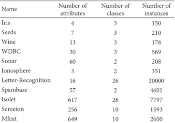
Table 1: Data sets used in the experiments. Name Number of attributes Number of classes Number of instances Iris 4 3 150 Seeds 7 3 210 Wine 13 3 178 WDBC 30 3 569 Sonar 60 2 208 Ionosphere _{3 2 351} Letter-Recognition 16 26 20000 Spambase 57 2 4601 Isolet 617 26 7797 Semeion 256 10 1593 Mfeat 649 10 2600

are always with high 𝑑 and 𝑛. Thus, using the traditional

SVD method will lead to enormous computation. Moreover, in this online metric learning model, the instances cannot be obtained at the orthogonal basis building step, which is regarded as a preprocess of the proposed method. Therefore, an online SVD algorithm should be introduced in our

framework. We use a truncated incremental SVD [19, 20]

to obtain the basis in our algorithm, which can decline the

computational complexity to 𝑂(𝑛𝑘3); when 𝑘 ≪ 𝑑, the

truncated incremental SVD algorithm will sharply reduce the computation time compared with traditional SVD algorithm. There are two main constraints for the regularization

parameter 𝜂_𝑡. First, it is used to make sure that 𝐹_𝑡+1

is a PSD matrix in each iteration. When 0 < 𝜂_𝑡 <

1/tr((𝐼 − 𝑀_𝑡)−1𝑀_𝑡𝑞_𝑡𝑞𝑇_𝑡), the 𝐹_𝑡+1 will be a PSD matrix

if 𝐹_𝑡 is a PSD matrix. This satisfies the first constraint.

Second, it also controls the balance of the regularization function and the loss function. In this paper, we select

𝜂𝑡 = 𝛼/tr((𝐼 − 𝑀𝑡)−1𝑀𝑡𝑞𝑡𝑞𝑇𝑡), where𝛼 is the learning rate

parameter which is chosen between0and1. On one hand, if

𝛼is too large, the𝐹_𝑡+1will be mainly updated to minimize the

loss function and satisfy the target relationship in the current triplet, which will lead to an unstable learning process. On

the other hand, if𝛼is too small, each iteration will have little

influence on the updating of the Mahalanobis matrix. Thus, the metric learning process will be very slow and insufficient.

Therefore, the selection of 𝛼 should consider the tradeoff

between efficiency and stability at the same time.

4. Experiments Results

In this section, we conduct experiments on several public domain data sets selected from UCI machine learning

reposi-tory (http://archive.ics.uci.edu/ml/) to present the superiority

of the proposed online LDML algorithm and the relationship between the performance and parameters. The parameters of

these benchmarks are listed inTable 1. Some of them are with

normal size while others have numerous instances or high dimension.

All the following experiments are tested in MATLAB 2011b, and all tests are implemented on a computer with Intel(R) Core(TM) i3-3120 M, 2.50 GHz CPU, 4G RAM, and Windows 7 operating system. The performance index is

chosen as the classification accuracy of𝑘-nearest neighbor.

The performance of all these algorithms is evaluated using 5-fold cross validation and the final results are the average of results obtained over 5 runs. In our proposed algorithm, when a new instance is recieved, it will be utilized to randomly build 2 triplets with instances which has been

received before. Thus, the total number of the triplets is2𝑛.

Meanwhile, the learning rate parameter is set as𝛼 = 1/2𝑛,

indicating that each triplet plays the same role in updating the Mahalanobis matrix.

The first experiment aims at illustrating the performance of the proposed compressed representation method in our online LDML algorithm. In this experiment, we try to use various compressed representation with different dimension-ality in the metric learning process. The experiments are, respectively, conducted on 3 selected data sets, including “WDBC,” “Sonar,” and “Ionosphere.” The dimensions of these three data sets are 30, 60, and 34. In this test, the number

of compressed dimensions varies from1 to the maximum

dimension of the data sets. The cross validation classification precision and the running time which change with the

number of dimensions are recorded. AndFigure 1gives the

relationship among these three items. We can see that the running time increases exponentially while the precision stays relatively constant when dimensions reach a certain value. The reason for this phenomenon can be explained

as follows. Although the Mahalanobis matrix𝑀is used to

build the relationship between features and the categories of instances, only a small part of elements in Mahalanobis

matrix𝑀make sense. Thus, using a low-rank Mahalanobis

matrix𝐹to represent the original𝑀is enough. It is worth

noting that if the rank of 𝐹 is too low, the accuracy will

decrease because𝐹does not have enough elements to retain

all the important information in metric learning process. In the second experiment, we compare the proposed method with many other basic classification methods and the state-of-the-art online metric learning algorithms, including

Euclidean distance, offline LDML [21], LEGO [13], online

ITML [7], and POLA [12]. The experiments are, respectively,

conducted on 6 data sets in UCI machine learning repository, including “Iris,” “Wine,” “WDBC,” “Seeds,” “Sonar,” and “Ionosphere.” These data sets are with normal dimension and number of instances. The testing results on cross validation classification accuracy for all data sets are summarized in

Table 2. The results list the average and stand deviation of the cross validation classification accuracy over 5 runs. Meanwhile, the number of the compressed dimensions in the proposed online LDML method is also presented in the brackets. From the comparisons we can see, the proposed method outperforms other online metric learning methods as well as Euclidean distance. The precision and robustness of the proposed method are better than all other online metric learning methods. At the same time, compared with the offline LDML, the proposed method only loses a

0 5 10 15 20 25 30 92 93 94 95 Number of dimensions A verag e c lassifica tio n p recisio n (%) 0 5 10 A verag e r unnin g time (s) (a) 0 5 10 15 20 25 30 35 86 88 A verag e c lassifica tio n p recisio n (%) Number of dimensions 0 2 4 A verag e r unnin g time (s) (b) 0 10 20 30 40 50 60 80 82 84 A verag e c lassifica tio n p recisio n (%) Number of dimensions 0 1 2 A verag e r unnin g time (s) (c)

Figure 1: The relationship among the number of dimensions, average classification precisions, and average running times. (a) The experiment results on data set “WDBC;” (b) the experiment results on dataset “Ionosphere;” (c) the experiment results on data set “Sonar.”

Table 2: Cross validation classification accuracy comparison with the state-of-the-art metric learning methods on the normal size data sets. Dataset Offline LDML Proposed LEGO Online ITML POLA Euclidean

Iris 0.9800 ± 0.0072 0.9760 ± 0.0037(2) 0.9653 ± 0.0087 0.9507 ± 0.0118 0.9600 ± 0.0166 0.9362 ± 0.0117 Wine 0.9551 ± 0.0221 0.9461 ± 0.0152(9) 0.9132 ± 0.0197 0.7832 ± 0.0228 0.7536 ± 0.0342 0.7427 ± 0.0447 Seeds 0.9543 ± 0.0051 0.9352 ± 0.0062(4) 0.8933 ± 0.0112 0.8760 ± 0.0137 0.8630 ± 0.0152 0.8762 ± 0.0085 WDBC 0.9469 ± 0.0031 0.9438 ± 0.0064(4) 0.9336 ± 0.0029 0.8332 ± 0.0216 0.8822 ± 0.0251 0.8891 ± 0.0202 Sonar 0.8384 ± 0.0120 0.8279 ± 0.0023(10) 0.8250 ± 0.0143 0.8365 ± 0.0186 0.7981 ± 0.0359 0.7240 ± 0.0079 Ionosphere 0.8946 ± 0.0060 0.8803 ± 0.0100(13) 0.8547 ± 0.0122 0.8203 ± 0.0103 0.8131 ± 0.0176 0.8376 ± 0.0191

Table 3: Running time (s) comparison with the state-of-the-art metric learning methods on the normal size data sets.

Dataset Offline LDML Proposed LEGO Online ITML POLA

Iris 0.4557 0.0306(2) 0.0287 0.0293 0.1372 Wine 0.7019 0.0434(9) 0.0387 0.0399 0.2231 Seeds 0.8957 0.0420(4) 0.0407 0.0420 0.2756 WDBC 3.4414 0.1286(4) 0.1682 0.1620 1.0273 Sonar 1.9713 0.0586(10) 0.1304 0.1291 0.6433 Ionosphere 3.3469 0.1009(13) 0.1229 0.1247 1.0725

0 0.5 1 1.5 2 0 1 2 3 4 5 6 7 Number of instances A verag e r unnin g time (s) Proposed method LEGO ×104 (a) 0 100 200 300 400 500 600 700 0 5 10 15 20 25 30 35 40 45 Number of dimensions A verag e r u nnin g time (s) Proposed method LEGO (b)

Figure 2: The relationship among number of instances, number of dimensions, and average running times. (a) The relationship between number of instances and average running times on data set “Letter-Recognition;” (b) the relationship between number of dimensions and average running times on data set “Mfeat.”

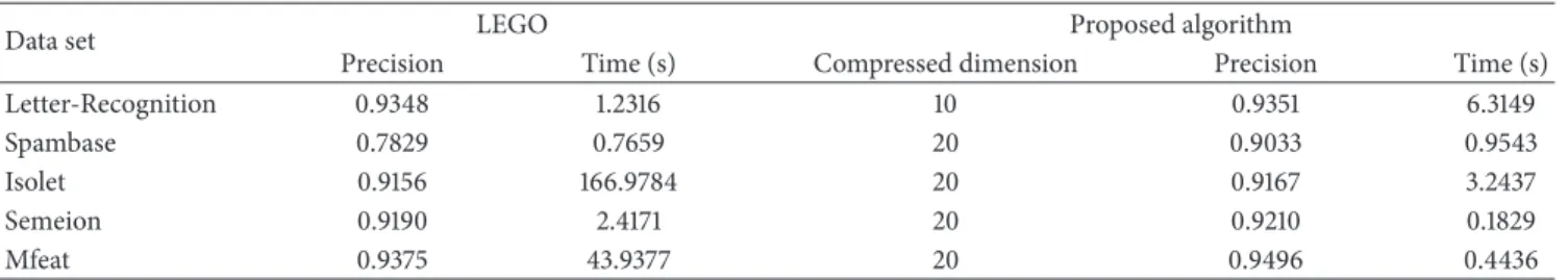
Table 4: Performance comparison with the state-of-the-art online metric learning methods on the large data sets.

Data set LEGO Proposed algorithm

Precision Time (s) Compressed dimension Precision Time (s)

Letter-Recognition 0.9348 1.2316 10 0.9351 6.3149

Spambase 0.7829 0.7659 20 0.9033 0.9543

Isolet 0.9156 166.9784 20 0.9167 3.2437

Semeion 0.9190 2.4171 20 0.9210 0.1829

Mfeat 0.9375 43.9377 20 0.9496 0.4436

the comparison of running time of these methods. We can see that the LEGO, online ITML, and the proposed method have comparable running times on the normal size data sets. However, our approach has a significant improvement of running time compared with the offline LDML method. Besides, the computational efficiency of the proposed method also outperforms that of POLA a lot.

Then, in the third experiment, tests are conducted on several large data sets to demonstrate the accuracy as well as efficiency of the online LDML algorithm. We select 5 large data sets from UCI machine learning repository, including “Letter-Recognition,” “Spambase,” “Isolet,” “Semeion,” and

“Mfeat.” From Table 1 we can see some of them contain

numerous instances while others are with high dimensional feature space. We mainly compare the proposed method with LEGO algorithm. The average accuracy and the average

running time are illustrated inTable 4. We can see that the

precisions of the proposed method on all data sets are better than that of LEGO, especially on the data set “Spambase.” When it comes to the running time, the performance of these two methods is totally different in different data sets. The LEGO algorithm runs fast on “Letter-Recognition” but

it has low efficiency on other data sets, including “Isolet” and “Mfeat.” However, the proposed method can reduce computational complexity on “Isolet” and “Mfeat” but it cannot run fast on “Letter-Recognition.” The reason of these phenomena is not obvious, and further experiments have been conducted to explain these findings.

In the following experiments, we test the relationship among number of instances, number of dimensions, and average running times. In this experiment, we firstly compare the changes of the running time when the number of instances increases. The experiment is conducted on the data

set “Letter-recognition” and the result is shown inFigure 2(a).

Although the running time of both methods is linear to the number of instances. The running time of the purposed time is a little faster than that of LEGO. The reason is that the

online LDML requires computing the orthogonal basis 𝑈.

Although we have applied the truncated incremental SVD to compute the orthogonal basis, the computational complexity

of truncated incremental SVD is𝑂(𝑛𝑘3). And it can reduce

running time sharply only when𝑘 ≪ 𝑑. However, in the

case of “Letter-Recognition,” the 𝑑 is 26 and 𝑘is 10. The

situation. Another experiment is to illustrate the changes of the running time when the number of dimensions increases. The experiment is conducted on the data set “Mfeat” and

the result is shown in Figure 2(b). In this experiment, we

gradually increase the feature dimension of the original data while online LDML only uses a 20 dimensional compressed representation all the time. We can see that the running time of proposed method stays of a very low value while that of LEGO increases the square of the number of feature dimensions. Therefore, the LEGO cannot deal with data sets with large feature dimension. The proposed method can reduce lots of computation time in each iteration while keeping high classification performance. This is the main advantage of the online LDML algorithm.

5. Conclusion

In this paper we propose a fast and robust metric learning algorithm for large data sets classification. Since large data sets usually contain numerous instances represented in high dimensional feature spaces, we propose to use an online Logdet divergence based metric learning model to improve the computation efficiency of learning with thousands of instances. Furthermore, we use a compressed representation of high dimensional Mahalanobis matrices to reduce the computational complexity in each iteration significantly. The proposed algorithm is shown to be efficient, robust, and precise by experiments on benchmark data sets and comparison with state-of-the-art algorithms. In future work we plan to further optimize the proposed algorithm with respect to computation efficiency and precision.

Conflict of Interests

The authors declare that there is no conflict of interests regarding the publication of this paper.

Acknowledgments

The research leading to these results has partially received funding from the Polish-Norwegian Research Programme operated by The National Centre for Research and Develop-ment under the Norwegian Financial Mechanism 2009–2014 in the frame of Project Contract no. Pol-Nor/200957/47/2013. Also, this work has been partially funded by the Research Council of Norway (RCN) under Grant 225231/O70.

References

[1] S. Yin, S. X. Ding, A. Haghani, H. Hao, and P. Zhang, “A comparison study of basic data-driven fault diagnosis and process monitoring methods on the benchmark tennessee eastman process,”Journal of Process Control, vol. 22, no. 9, pp. 1567–1581, 2012.

[2] S. Yin, G. Wang, and H. R. Karimi, “Data-driven design of robust fault detection system for wind turbines,”Mechatronics, 2013.

[3] S. Yin, S. X. Ding, A. H. Abandan Sari, and H. Hao, “Data-driven monitoring for stochastic systems and its application on batch process,”International Journal of Systems Science, vol. 44, no. 7, pp. 1366–1376, 2013.

[4] H. Gao, C. Ding, C. Song, and J. Mei, “Automated inspection of e-shaped magnetic core elements using k-tsl-center clustering and active shape models,” IEEE Transactions on Industrial Informatics, vol. 9, no. 3, pp. 1782–1789, 2013.

[5] M. Guillaumin, J. Verbeek, and C. Schmid, “Is that you? Metric learning approaches for face identification,” inProceedings of the IEEE 12th International Conference on Computer Vision (ICCV ’09), pp. 498–505, October 2009.

[6] E. P. Xing, M. I. Jordan, S. Russell, and A. Ng, “Distance metric learning with application to clustering with side-information,” inAdvances in Neural Information Processing Systems, pp. 505– 512, 2002.

[7] J. V. Davis, B. Kulis, P. Jain, S. Sra, and I. S. Dhillon, “Information-theoretic metric learning,” inProceedings of the ACM 24th International Conference on Machine Learning (ICML ’07), pp. 209–216, June 2007.

[8] P. Jain, B. Kulis, J. V. Davis, and I. S. Dhillon, “Metric and kernel learning using a linear transformation,” Journal of Machine Learning Research, vol. 13, pp. 519–547, 2012.

[9] K. Weinberger, J. Blitzer, and L. Saul, “Distance metric learning for large margin nearest neighbor classification,” inAdvances in Neural Information Processing Systems, vol. 18, p. 1473, 2006. [10] S. Yin, H. Luo, and S. Ding, “Real-time implementation of

fault-tolerant control systems with performance optimization,”IEEE Transactions on Industrial Electronics, vol. 61, no. 5, pp. 2402– 2411, 2012.

[11] J. V. Davis and I. S. Dhillon, “Differential entropic clustering of multivariate gaussians,” inAdvances in Neural Information Processing, pp. 337–344, 2006.

[12] S. Yin, X. Yang, and H. R. Karimi, “Data-driven adaptive observer for fault diagnosis,”Mathematical Problems in Engi-neering, vol. 2012, Article ID 832836, 21 pages, 2012.

[13] S. Shalev-Shwartz, Y. Singer, and A. Y. Ng, “Online and batch learning of pseudo-metrics,” inProceedings of the ACM 21st International Conference on Machine Learning (ICML ’04), p. 94, July 2004.

[14] P. Jain, B. Kulis, I. S. Dhillon, and K. Grauman, “Online metric learning and fast similarity search,” inProceedings of the 22nd Annual Conference on Neural Information Processing Systems (NIPS ’08), pp. 761–768, December 2008.

[15] B. Kulis, M. Sustik, and I. Dhillon, “Learning low-rank kernel matrices,” inProceedings of the 23rd International Conference on Machine Learning (ICML ’06), pp. 505–512, June 2006. [16] M. Sugiyama, “Dimensionality reduction of multimodal labeled

data by local fisher discriminant analysis,”Journal of Machine Learning Research, vol. 8, pp. 1027–1061, 2007.

[17] Q. Wang, P. C. Yuen, and G. Feng, “Semi-supervised metric learning via topology preserving multiple semi-supervised assumptions,”Pattern Recognition, vol. 46, no. 9, pp. 2576–2587, 2013.

[18] J. V. Davis and I. S. Dhillon, “Structured metric learning for high dimensional problems,” inProceedings of the 14th ACM SIGKDD International Conference on Knowledge Discovery and Data Mining (KDD ’08), pp. 195–203, August 2008.

[19] H. Zha and H. D. Simon, “On updating problems in latent semantic indexing,”SIAM Journal on Scientific Computing, vol. 21, no. 2, pp. 782–791, 1999.

[20] H. Zhao, P. C. Yuen, and J. T. Kwok, “A novel incremental principal component analysis and its application for face recog-nition,”IEEE Transactions on Systems, Man, and Cybernetics B: Cybernetics, vol. 36, no. 4, pp. 873–886, 2006.

[21] J. Mei, M. Liu, H. R. Karimi, and H. Gao, “Logdet divergence based metric learning using triplet labels,” inProceedings of the Workshop on Divergences and Divergence Learning ( ICML ’13), 2013.

Submit your manuscripts at

http://www.hindawi.com

Hindawi Publishing Corporation

http://www.hindawi.com Volume 2014

Mathematics

Hindawi Publishing Corporation

http://www.hindawi.com Volume 2014

Mathematical Problems in Engineering

Hindawi Publishing Corporation http://www.hindawi.com

Differential Equations International Journal of

Volume 2014 Hindawi Publishing Corporation

http://www.hindawi.com Volume 2014 Hindawi Publishing Corporationhttp://www.hindawi.com Volume 2014

Hindawi Publishing Corporation

http://www.hindawi.com Volume 2014 Mathematical PhysicsAdvances in

Complex Analysis

http://www.hindawi.com Volume 2014

Optimization

Hindawi Publishing Corporation

http://www.hindawi.com Volume 2014

Combinatorics

Hindawi Publishing Corporation

http://www.hindawi.com Volume 2014

International Journal of

Hindawi Publishing Corporation

http://www.hindawi.com Volume 2014

Journal of

Hindawi Publishing Corporation

http://www.hindawi.com Volume 2014

Function Spaces

Abstract and Applied Analysis

Hindawi Publishing Corporation

http://www.hindawi.com Volume 2014 International Journal of Mathematics and Mathematical Sciences

Hindawi Publishing Corporation http://www.hindawi.com Volume 2014

The Scientific

World Journal

http://www.hindawi.com Volume 2014

Hindawi Publishing Corporation

http://www.hindawi.com Volume 2014

Discrete Dynamics in Nature and Society Hindawi Publishing Corporation

http://www.hindawi.com Volume 2014 Hindawi Publishing Corporation

http://www.hindawi.com Volume 2014

Discrete Mathematics

Hindawi Publishing Corporation

http://www.hindawi.com Volume 2014 Hindawi Publishing Corporationhttp://www.hindawi.com Volume 2014

Stochastic Analysis