Robust methods based on shrinkage

(1)

Robust methods based on shrinkage

by

Elisa Cabana Garceran del Vall

Thesis submitted in partial compliance with the requirements for the

degree of Doctor of Philosophy in Mathematical Engineering

Universidad Carlos III de Madrid

Advisor:

Rosa Elvira Lillo Rodr´ıguez

(2)

(3)

To my family and friends,

“I have no special talent, I am only passionately curious.”

(4)

(5)

Acknowledgements

These are certainly the most difficult pages from this thesis I have to write. Not because I don’t know how to thank the people involved in this Ph.D. stage of my life, but because I think that I can write a whole book about it and it is hard to summarize all my gratefulness in a few pages. This has been quite a journey. It feels this is not enough, but I will try to do my best in expressing my most sincere appreciation.

First, I would like to thank the director of this piece of work, Rosa Elvira Lillo, my “work mother”, who adopted me and taught me to be pragmatic, proactive, effi-cient and consistent. I even felt like a robust estimator. Henry Laniado contributed also to this thesis. He was the first person I asked about research in my early stages, and since he was working together with Rosa in this topic they both captured me to work with them. I am grateful for all of their advices and for encouraging me to join them.

Next, I have to thank my real mother Mar´ıa Eugenia for always being there, despite the 7432𝑘𝑚 that have separated us the last six years. Her support is what has sustained me in my worst moments. My dad is now closer than it was most of my life, for that I am truly grateful. I would like to take advantage of these lines to say what I never say out loud but I have always thought: thank you both for giving me life and for all your help so I could get here and fulfill my dreams when the situation was difficult.

When I came to Spain to do the master, it was my first trip out of the bub-ble that Cuba is. I had no idea I would spend so many years in this university. I had no clue that I was capable of research, creating new methods, or teaching Statistics to freshman students. Thanks to the Department, I had the possibility to share my knowledge and meet new people in several congresses and for that, I am really grateful. I also had difficulties on the way, but I consider that they made me stronger. Now all those challenges and struggles, all the never give up and I cannot surrender, are the true victory. But the most significant of my experience these years, is the friendship of my closest friends. Vero, my sister in soul, who has

(6)

been a huge support from the beginning. Alba, MJ, Rub´en and Ma˜nas, my dearest friends, without them the two years of the master would never have been the same; I will never forget all of our shafiness and our adventures. Fer, the one who has been by my side these last three years, holding my cries, my cravings, my fears, my worst moments, and even then, he has managed to help me create my best version of myself. I have infinite gratitude towards him and his family, for making me feel like home.

Finally, I want to acknowledge the financial support received from the Spanish Ministry of Economy and Competitiveness ECO2015-66593-P and the UC3M PIF pre-doctoral scholarship.

(7)

Published and submitted contents

Published contents:

E. Cabana, Rosa E. Lillo, H. Laniado. Multivariate outlier detection based on a robust Mahalanobis distance with shrinkage estimators. UC3M Working Papers Statistics and Econometrics, 27-10, 2017. https://e-archivo.uc3m. es/handle/10016/24613

– Co–author.

– It is partially included in Chapters 2 and 3 of the thesis.

– The material from this source included in the thesis is not indicated by typographical means or references.

E. Cabana, Rosa E. Lillo, H. Laniado. Shrinkage reweighted regression. UC3M Working papers Statistics and Econometrics, 19-08, 2019. https://e-archivo. uc3m.es/handle/10016/28500

– Co–author.

E. Cabana, Rosa E. Lillo, H. Laniado. Multivariate outlier detection based on a robust Mahalanobis distance with shrinkage estimators. ArXiv, 2019.

https://arxiv.org/abs/1904.02596

– Co–author.

E. Cabana, Rosa E. Lillo, H. Laniado. Robust regression based on shrinkage estimators. ArXiv, 2019. https://arxiv.org/abs/1905.02962

– Co–author.

(8)

Contents submitted for publication:

E. Cabana, Rosa E. Lillo, H. Laniado. Multivariate outlier detection based on a robust Mahalanobis distance with shrinkage estimators. 2019. Statistical Papers.

– Co–author.

E. Cabana, Rosa E. Lillo, H. Laniado. Robust regression based on shrinkage with application to Living Environment Deprivation. 2019. Stochastic Envi-ronmental Research and Risk Assessment.

– Co–author.

(9)

Abstract

In this thesis, robust methods based on the notion ofshrinkage are proposed for out-lier detection and robust regression. A collection of robust Mahalanobis distances is proposed for multivariate outlier detection. The robust intensity and scaling factors, needed to define the shrinkage of the robust estimators used in the distances, are op-timally estimated. Some properties are investigated, such as the affine equivariance and the breakdown value. The performance of the proposal is illustrated through the comparison to other robust techniques from the literature, in a simulation study and with a real example of breast cancer data. The robust alternatives are also reviewed, highlighting their advantages and disadvantages. The behavior when the underlying distribution is heavy-tailed or skewed, shows the appropriateness of the proposed method when we deviate from the common assumption of normality. The resulting high true positive rates and low false positive rates in the vast majority of cases, as well as the significantly smaller computational time show the advantages of the proposal.

On the other hand, a robust estimator is proposed for the parameters that char-acterize the linear regression problem. It is also based on the notion of shrinkages. A thorough simulation study is conducted to investigate the efficiency with Normal and heavy-tailed errors, the robustness under contamination, the computational times, the affine equivariance and breakdown value of the regression estimator. It is compared to the classical Ordinary Least Squares (OLS) approach and the robust alternatives from the literature, which are also briefly reviewed in the thesis. Two classical data-sets often used in the literature and a real socio-economic data-set about the Living Environment Deprivation (LED) of areas in Liverpool (UK), are studied. The results from the simulations and the real data examples show the advantages of the proposed robust estimator in regression. Also, with the LED data-set it is also shown that the proposed robust regression method has improved performance than machine learning techniques previously used for this data, with the advantage of interpretability.

Furthermore, an adaptive threshold, that depends on the sample size and the dimension of the data, is introduced for the proposed robust Mahalanobis distance

(10)

based on shrinkage estimators. The cut-off is different than the classical choice of the 0.975 chi-square quantile providing a more accurate method to detect multivari-ate outliers. A simulation study is done to check the performance improvement of the new cut-off against the classical. The adjusted quantile shows improved per-formance, even when the underlying distribution is heavy-tailed or skewed. The method is illustrated using the LED data-set, and the results demonstrate the ad-ditional advantages of the adaptive threshold for the regression problem.

(11)

Resumen

En esta tesis, se proponen métodos robustos basados en la noción de shrinkage para la detección de at´ıpicos y la regresión robusta. Se propone una colección de dis-tancias de Mahalanobis robustas para la detección de outliers multivariantes. Los factores de intensidad y escala, necesarios para definir el shrinkage de los estimadores robustos utilizados en las distancias, se estiman de manera óptima. Se investigan algunas propiedades como la equivarianza af´ın y el breakdown value (valor de rup-tura). El desempeño de la propuesta se ilustra mediante la comparación con otras técnicas robustas de la literatura, en un estudio de simulación y con un ejemplo real de datos de cáncer de mama. Las alternativas robustas también se revisan, destacando sus ventajas y desventajas. El comportamiento cuando la distribución subyacente es de cola pesada o asimétrica, muestra lo apropiado que es el método propuesto cuando nos apartamos de la suposición común de normalidad. Las altas tasas de verdaderos positivos y las bajas tasas de falsos positivos, en la gran mayor´ıa de los casos, as´ı como el tiempo de cómputo significativamente menor, muestran las ventajas de la propuesta.

Por otro lado, se introduce un estimador robusto para los parámetros que ca-racterizan la regresión lineal. También se basa en la noción de shrinkage. Se lleva a cabo un estudio de simulación exhaustivo para investigar la eficiencia con erro-res Normales y de cola pesada, la robustez bajo contaminación, los tiempos de cómputo, la equivarianza af´ın y el valor de ruptura del estimador de regresión. Se compara con el método M´ınimos Cuadrados Ordinarios (OLS) clásico y las alter-nativas sólidas de la literatura, que también se revisan brevemente en la tesis. Se estudian dos conjuntos de datos clásicos que se utilizan a menudo en la literatura y un conjunto de datos socioeconómicos reales sobre la privación del entorno vital (LED) de las áreas de Liverpool (Reino Unido). Los resultados de las simulaciones y los ejemplos de datos reales muestran las ventajas del estimador robusto propuesto para regresión. Además, con el conjunto de datos LED también se muestra que el método de regresión robusta propuesto presenta mejoras con respecto a las técnicas de aprendizaje automático utilizadas anteriormente para estos datos, con la ventaja de la interpretabilidad.

(12)

Además, se introduce un recorte adaptativo, que depende del tamaño de la mues-tra y la dimensión de los datos, para la distancia robusta de Mahalanobis propuesta, basada en estimadores shrinkage. El valor de recorte es diferente a la opción clásica del cuantil 0.975 de la chi-cuadrado, y proporciona un método más preciso para detectar valores at´ıpicos multivariados. Se realiza un estudio de simulación para verificar el rendimiento del nuevo punto de corte respecto al clásico. El cuantil ajus-tado muestra un desempeño mejorado, incluso cuando la distribución subyacente es de cola pesada o asimétrica. El método se ilustra utilizando el conjunto de datos LED y los resultados demuestran las ventajas adicionales del recorte adaptativo para el problema de regresión.

(13)

Contents

Acknowledgements i

Published and submitted contents iii

Abstract v

Resumen vii

1 Introduction 21

1.1 Structure of the thesis . . . 25

2 Robust outlier detection 27 2.1 Minimum Covariance Determinant (MCD) . . . 27

2.2 Adjusted Minimum Covariance Determinant (Adj MCD) . . . 29

2.3 Kurtosis . . . 30

2.4 Orthogonalized Gnanadesikan-Kettenring (OGK) . . . 31

2.5 Comedian . . . 32

2.6 Summary . . . 33

3 Robust outlier detection based on shrinkage 35 3.1 Location parameter . . . 35

3.2 Dispersion parameter . . . 38

3.3 Proposed Robust Mahalanobis Distances . . . 41

3.4 Simulation results . . . 41

3.4.1 Normal distribution . . . 41

3.4.2 𝑡3-distribution . . . 43

3.4.3 Exponential distribution . . . 44

3.4.4 Summary and selection of one of our proposed distances . . . 44

3.5 Properties of the estimator . . . 45

3.5.1 Correlation and affine equivariance . . . 45

3.5.2 Breakdown value . . . 48

3.5.3 Computational times . . . 49

(14)

3.7 Summary . . . 53

4 Robust regression 55 4.1 Least Absolute Deviation (LAD) regression . . . 55

4.2 M-estimator . . . 56

4.3 R-estimator . . . 56

4.4 Generalized M-estimator . . . 57

4.5 Least Median of Squares (LMS) regression . . . 57

4.6 Least Trimmed Squares (LTS) regression . . . 57

4.7 S-estimator . . . 58

4.8 Generalized S-estimator . . . 58

4.9 MM-estimates . . . 58

4.10 Covariance approach . . . 58

4.11 Robust and efficient weighted least square (REWLSE) . . . 59

4.12 Summary . . . 59

5 Robust regression based on shrinkage 61 5.1 Shrinkage reweighted regression estimator . . . 61

5.2 Simulation structure . . . 63 5.3 Efficiency . . . 64 5.4 Robustness . . . 66 5.4.1 Computational times . . . 70 5.5 Equivariance properties . . . 71 5.6 Breakdown property . . . 73

5.7 Real data-set examples . . . 74

5.7.1 Star data . . . 74

5.7.2 Hawkins-Bradu-Kass data . . . 76

5.7.3 Living Environment Deprivation data . . . 76

5.8 Summary . . . 82

6 Adjusted quantile 83 6.1 Estimating the adjusted threshold . . . 84

6.2 Simulations . . . 87

6.2.1 Normal distribution . . . 87

6.2.2 𝑡3-distribution . . . 89

6.2.3 Exponential distribution . . . 91

6.3 Real data-set example . . . 92

6.4 Summary . . . 94

7 Conclusions and Future research lines 97 7.1 Future work . . . 98

Appendix A Proofs from Chapter 3 103 A.1 Proof of Proposition 1. . . 103

A.2 Proof of Proposition 2. . . 104

(15)

Contents xi

Appendix B Tables from Chapter 3 107

B.1 Normal distribution . . . 107 B.2 Multivariate Student-t distribution with 3 d.g. . . 113 B.3 Multivariate Exponential distribution . . . 117

Appendix C Figures from Chapter 3 119

Appendix D Tables from Chapter 5 131

(16)

2.1 Star data with 97.5% tolerance ellipses corresponding to MD and RMD.. . . 28

3.1 Standardized data with the “multivariate boxplot”. . . 50

3.2 Some of the alternative methods detected outliers belonging to the 50% of the most central data. . . 52

3.3 RMD-S detected outliers that belong to the 50% of the most central data. . . 52

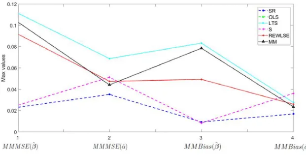
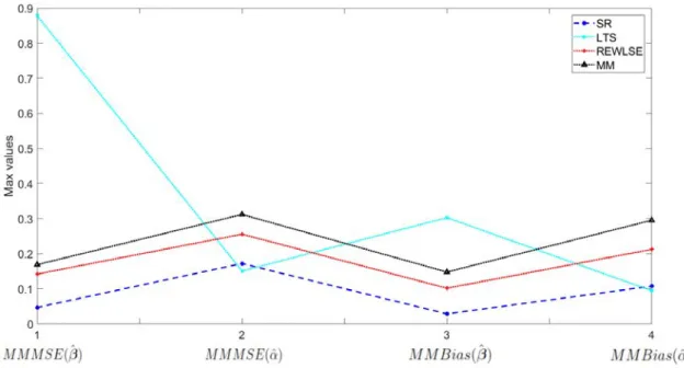
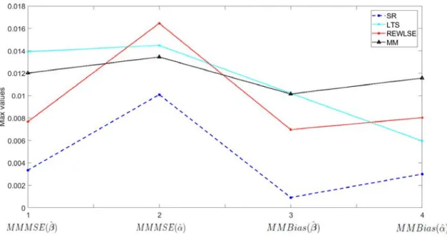
5.1 𝑀 𝑀 𝑆𝐸( ^𝛽) with 𝑝= 5, 𝑛= 100, 𝛿= 10%. . . 66

5.2 (Zoom) 𝑀 𝑀 𝑆𝐸( ^𝛽) with 𝑝= 5, 𝑛= 100, 𝛿= 10%. . . 67

5.3 𝑀 𝑀 𝑀 𝑆𝐸 and 𝑀 𝑀 𝐵𝑖𝑎𝑠, with 𝑝= 5, 𝑛= 100 and 𝛿 = 10%. . . 67

5.4 (Zoom) 𝑀 𝑀 𝑀 𝑆𝐸 and 𝑀 𝑀 𝐵𝑖𝑎𝑠, with 𝑝= 5 and𝛿= 10%. . . 68

5.5 𝑀 𝑀 𝑀 𝑆𝐸 and 𝑀 𝑀 𝐵𝑖𝑎𝑠, with 𝑝= 5 and𝛿 = 20%. . . 68

5.6 (Zoom) 𝑀 𝑀 𝑀 𝑆𝐸 and 𝑀 𝑀 𝐵𝑖𝑎𝑠, with 𝑝= 5 and𝛿= 20%. . . 69

5.7 𝑀 𝑀 𝑀 𝑆𝐸 and 𝑀 𝑀 𝐵𝑖𝑎𝑠, with 𝑝= 30 and 𝛿= 10%. . . 69

5.8 (Zoom) 𝑀 𝑀 𝑀 𝑆𝐸 and 𝑀 𝑀 𝐵𝑖𝑎𝑠, with 𝑝= 30 and 𝛿= 10%. . . 70

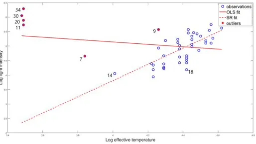
5.9 Star data-set with OLS and SR regression fit. . . 75

5.10 Correlation matrix for LED index data-set. . . 77

5.11 Cross-validated 𝑅2 and median values (dashed line), with pca. . . 79

5.12 Cross-validated MSE and median values (dashed line), with pca. . . . 79

5.13 Cross-validated 𝑅2 _{. . . 80}

5.14 Cross-validated MSE . . . 80

5.15 Cross-validated𝑅2 _{and median values (dashed line), for both pca and} spca. . . 81

6.1 Simulated 𝑝𝑛(𝛿) for multivariate Normal distributions with different sample sizes (𝑥−axis) and dimensions𝑝≤10. . . 85

6.2 Slopes of lines from Figure 6.1 plotted against dimension 𝑝. . . 86

6.3 Simulated 𝑝𝑛(𝛿) for multivariate Normal distributions with different sample sizes (𝑥−axis) and dimensions𝑝 > 10. . . 86

6.4 Slopes of lines from Figure 6.3 plotted against dimension 𝑝. . . 87

6.5 Cross-validated 𝑅2_{. . . 93}

(17)

List of figures xiii

7.1 fMRI scan. . . 100

C.1 Standardized data with the “multivariate boxplot”. . . 119

C.2 Detected outliers by MCD. . . 119

C.3 Detected outliers by Adjusted MCD. . . 120

C.4 Detected outliers by Kurtosis.. . . 120

C.5 Detected outliers by OGK. . . 120

C.6 Detected outliers by COM. . . 121

C.7 Detected outliers by RMD-S. . . 121

C.8 MCD detected outliers that belong to the 50% of the most central data. . . 121

C.9 MCD detected outliers that belong to the 50% of the most central data. . . 122

C.10MCD detected outliers that belong to the 50% of the most central data. . . 122

C.11Adjusted MCD detected outliers that belong to the 50% of the most central data. 122 C.12Adjusted MCD detected outliers that belong to the 50% of the most central data. 123 C.13Adjusted MCD detected outliers that belong to the 50% of the most central data. 123 C.14Kurtosis detected outliers that belong to the 50% of the most central data. . . . 123

C.15Kurtosis detected outliers that belong to the 50% of the most central data. . . . 124

C.19OGK detected outliers that belong to the 50% of the most central data. . . 126

C.24Comedian detected outliers that belong to the 50% of the most central data. . . 128

C.25Comedian detected outliers that belong to the 50% of the most central data. . . 129

(18)

3.1 Combinations of location and dispersion . . . 41

3.2 True positive rates, with Normal distribution. . . 43

3.3 True positive rates, with Normal distribution. . . 43

3.4 Simulation results for correlated data. . . 46

3.5 True posive rates and false positive rates of RMD-S for transformed data, 𝜆= 0.1. . . 47

3.6 True posive rates and false positive rates of RMD-S for transformed data, 𝜆= 1. . . 47

3.7 Simulation results for breakdown value. . . 48

3.8 Computational times with Normal data, 𝛿= 5 and 𝜆= 0.1. . . 49

3.9 Detected outliers inside and outside the fences. . . 51

3.10 Detected outliers inside the “box” with the 50% of the most central data. . . 51

3.11 Computational times for each method with the WDBC data-set. . . . 53

5.1 Finite sample efficiency in case of Normal errors, scenario [NE] . . . . 65

5.2 MSE in case of 𝑡−student distributed errors, scenario [TE] . . . 65

5.3 Computational times with Normal distribution 𝑝= 5 and𝑛= 100 . . 70

5.4 Computational times with Normal distribution 𝑝= 30 and 𝑛= 500 . 70 5.5 𝑀 𝑀 𝑆𝐸𝜆( ^𝜙𝑆𝑅𝑛𝑒𝑤) for regression and y-equivariance . . . 72

5.6 𝑀 𝑀 𝑆𝐸𝜆( ^𝜙𝑆𝑅𝑛𝑒𝑤) for x-equivariance . . . 73

5.7 MMMSE and MMBias, 𝑝= 5 . . . 73

5.8 MMMSE and MMBias, 𝑝= 30 . . . 74

5.9 Estimation of intercept and slope and detected outliers with star data. 75 5.10 𝑅2 _{for each method with stars data-set. . . 76}

5.11 Estimation of the parameters and detected outliers with HBK data. . 76

5.12 Adjusted𝑅2 _{for each method with HBK data-set. . . 76}

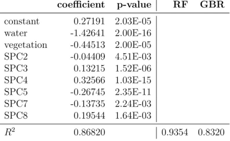
5.13 𝑅2 _{with (pca transformed) LED index data-set. . . 78}

5.14 Median cross-validated𝑅2 _{with (pca transformed) LED index data-set. 79} 5.15 Median cross-validated 𝑅2_{. . . 81}

5.16 Results for the model estimated by SR with spca transformation and the 𝑅2 for RF and GBR. . . 81

(19)

List of tables xv

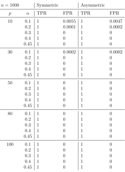
6.1 FPR for Normal data with 𝛼= 0%. . . 88

6.2 𝐹−scores in case of Normal data. . . 88

6.3 FPR for 𝑡3-distributed data with𝛼 = 0%. . . 89

6.4 𝐹−scores in case of 𝑡3-distributed data. . . 90

6.5 FPR for exponential distributed data with 𝛼 = 0%. . . 91

6.6 𝐹−scores in case of exponential distributed data. . . 91

6.7 𝑅2 measures. . . 92

6.8 Median cross-validated 𝑅2_{. . . 93}

6.9 Results for the model estimated by SR with spca transformation and the 𝑅2 for RF and GBR. . . 94

B.1 False positive rates with Normal distribution 𝛼= 0. . . 107

B.2 True positive rates with Normal distribution. . . 108

B.3 True positive rates with Normal distribution. . . 109

B.4 False positive rates with Normal distribution. . . 110

B.5 False positive rates with Normal distribution. . . 111

B.6 Computational times with Normal data 𝛿 = 5 and𝜆= 1. . . 111

B.7 Computational times with Normal data 𝛿 = 10 and 𝜆= 0.1. . . 112

B.8 Computational times with Normal data 𝛿 = 10 and 𝜆= 1. . . 112

B.9 False positive rates with Student-t distribution with 3 d.f, 𝛼= 0. . . . 113

B.10 True positive rates with Student-t distribution with 3 d.f. . . 113

B.11 True positive rates with Student-t distribution with 3 d.f. . . 114

B.12 False positive rates with Student-t distribution with 3 d.f. . . 115

B.13 False positive rates with Student-t distribution with 3 d.f. . . 116

B.14 False positive rates with Exponential distribution,𝛼 = 0. . . 117

B.15 True positive rates with Exponential distribution. . . 117

B.16 False positive rates with Exponential distribution. . . 118

D.1 MMMSE and MMBias of ^𝛽 and ^𝛼, for 𝑝= 5 and 𝛿= 10%. . . 131

(20)

(21)

CHAPTER

1

Introduction

The detection of outliers in multivariate data is an important task in Statistics since that kind of observations can distort any statistical procedure. In data mining and machine learning contexts, many standard techniques such as principal compo-nent analysis and linear discriminant analysis are inherently susceptible to atypical observations (Tarr et al. [2016]). The task of detecting multivariate outliers can be useful in various fields (Vargas N [2003], Brettschneider et al. [2008], Hubert et al.[2008],Hubert and Debruyne [2010],Perrotta and Torti[2010] and Choi et al.

[2016]). However, nowadays, there are several real situations from the outlier detec-tion field, in which the data contains a large number of variables. For example, in neuroimaging, data almost surely contains rare observations due to problems like ac-quisition, pre-processing artifacts, or inter-subject variability. Functional Magnetic Resonance Imaging (fMRI) is a concrete example. In the analysis of fMRI data, even small movements of the head of the patients, or even the subject’s heartbeat and breathing, may produce large artifacts in the signals and noise directly in the data (Wager et al. [2005], Lazar [2008], Lindquist [2008],Monti [2011], Poline and Brett

[2012]). High-dimensional data are increasingly encountered in other applications of statistics, e.g., in biological and financial studies (Chen et al. [2010] andZeng et al.

[2015]), and also geochemical data (Reimann and Filzmoser [2000], Templ et al.

[2008]), which practically always contains outliers.

The definition of outlier is not unique, but they are generally defined as ob-servations resulting from a secondary process, which differs from the background distribution. This kind of data does not need to be especially high or low concern-ing all values of the variables in the data-set. Thus, this is the reason why the task of identifying multivariate outliers with the classical univariate methods commonly fail. In the multivariate case, there must be considered both the distance of an ob-servation from the centroid of the data, and the shape of the data. The covariance matrix characterizes the shape of multivariate observations, and the Mahalanobis distance (MD) (seeMahalanobis[1936]) is a well-known measure which takes it into account.

(22)

The classical Mahalanobis distance is defined for every 𝑝−dimensional observa-tion x𝑖 of the multivariate sample {x1, ...,x𝑛}, as:

𝑀 𝐷(x𝑖) =

(︁

(x𝑖−𝜇^) ^Σ−1(x𝑖−𝜇^) 𝑡)︁1/2

,

where ^𝜇is the estimated multivariate location (sample mean) and ^Σ is the estimated covariance matrix (sample covariance matrix).

The problem with this definition is that the classical estimates of location and covariance matrix are often highly influenced by the presence of outliers (Rousseeuw et al.[1986],Rousseeuw and Van Zomeren[1990]). This means that a single extreme observation or groups of observations, departing from the main data structure can have a high influence on the distance measure. Two problems can arise, there might be outliers with not a large MD value, which is called amasking problem, and not all observations with large MD values are necessarily outliers, which is calledswamping problem (Hadi [1992]). The problems of masking and swamping arise due to the influence of outliers on classical location and scatter estimates (sample mean and sample covariance matrix), which implies that the estimated distance will not be robust. The solution is to consider robust estimators to obtain a robust Mahalanobis distance (RMD): 𝑅𝑀 𝐷(x𝑖) = (︁ (x𝑖 −𝜇^𝑅) ^Σ −1 𝑅 (x𝑖 −𝜇^𝑅) 𝑡)︁1/2 , (1.1)

where ^𝜇_𝑅 and ^Σ𝑅 are robust estimators of centrality and covariance matrix, respec-tively.

For multivariate normally distributed data, the distribution of the classical squared Mahalanobis distance,𝑀 𝐷2, is known (Gnanadesikan and Kettenring [1972]) to be chi-squared with 𝑝 (the dimension of the data) degrees of freedom, i.e., 𝜒2

𝑝. Then, the adopted rule for identifying the outliers is selecting the threshold as the 0.975 quantile of the 𝜒2_𝑝. However, the squared RMD does not necessarily follow a chi-squared distribution when the data are not Gaussian distributed. Thus, determining exact cut-off values for outlying distances continues to be a difficult problem and has found much attention because no universally applicable method has been pro-posed. Despite this fact, the 𝜒2

𝑝;0.975 quantile is often considered as the threshold for recognizing outliers in the robust distance case, but this approach may have some drawbacks. Evidence of this behavior is now well documented even in mod-erately large samples, especially when the number of dimensions increases (Becker and Gather [1999], Hardin and Rocke [2005], Cerioli et al. [2009] and Riani et al.

[2008]).

On the other hand, one special case in the multivariate space is the linear regres-sion problem, which is widely used in numerous fields. Consider the linear regresregres-sion model:

(23)

Chapter 1. Introduction 23

for𝑖= 1, ..., 𝑛, where𝑛 is the sample size, 𝛼 is the unknown intercept, 𝛽 is the un-known (𝑝×1) vector of regression parameters, the error terms 𝜖𝑖 are i.i.d and they are also independent from the 𝑝-dimensional carriers x𝑖 (often also called regressor or explanatory variables).

The classical approach to estimate the parameters of the model is the Ordinary Least Squares (OLS) estimator of Gauss and Legendre, which minimizes the sum of squared residuals: ^ 𝛽_𝑂𝐿𝑆 =𝑎𝑟𝑔𝑚𝑖𝑛 𝛽 𝑛 ∑︁ 𝑖=1 (𝑦𝑖−x𝑡𝑖𝛽) 2 . (1.2)

However, OLS estimator is not robust to the presence of outliers. The efficiency and breakdown point (bdp) are two traditionally used criteria to compare the ex-isting robust methodologies. Since OLS has the smallest variance among unbiased estimates when the errors are normally distributed, and there are no outliers, in this scenario, OLS has maximum efficiency. Thus, the relative efficiency of the ro-bust estimate compared to OLS when the error distribution is exactly Normal, and the data is clean, is often considered as a measure to study the performance of the methods and to compare them with each other. The bdp measures the proportion of outliers an estimate can tolerate. Usually, the definition offinite sample bdp is used (Donoho and Huber [1983]). Given any sample z = (z1, ...,z𝑛), with z𝑖 = (x𝑖, 𝑦𝑖), wherex𝑖 is of dimension 1×𝑝, for all 𝑖= 1, ..., 𝑛, denote by 𝑇(z) an estimate of the parameter𝛽. Let_̃︀z be the corrupted sample where any𝑞 of the original points ofz are replaced by arbitrary outliers. Then the finite sample bdp 𝛾* is defined as:

𝛾*(𝑇,z) = 𝑚𝑖𝑛 1≤𝑞≤𝑛{ 𝑞 𝑛 :𝑠𝑢𝑝 ̃︀ 𝑧 ||𝑇(_̃︀z)−𝑇(z)||=∞},

where || · || is the Euclidean norm. The asymptotic bdp is understood as the limit of the finite sample bdp when𝑛 goes to infinity. Intuitively, the maximum possible asymptotic bdp is 1/2 because if more than half of the observations are contami-nated, it is not possible to distinguish between the background data and the con-tamination (Leroy and Rousseeuw[1987]). OLS has a finite sample bdp of 1/𝑛, i.e., the occurrence of even a single outlier can affect the results drastically. Therefore, its asymptotic bdp is 0.

OLS estimator can be alternatively expressed as follows. Denote the joint vari-able of the response and carriers as z= (x,y). Denote the location of z by 𝜇 and the scatter matrix by Σ. Partitioning 𝜇and Σ yields the notation:

𝜇= (︂ 𝜇_𝑥 𝜇𝑦 )︂ , Σ = (︂ Σ𝑥𝑥 Σ𝑥𝑦 Σ𝑦𝑥 Σ𝑦𝑦 )︂ .

Traditionally they are estimated by the empirical mean ^𝜇 and the empirical covariance matrix ^Σ. OLS estimators of 𝛽 and the intercept 𝛼 can be written as functions of the components of𝜇^ and ^Σ, namely

^

𝛽= ^Σ−_𝑥𝑥1Σ^𝑥𝑦, 𝛼^= ^𝜇𝑦 −𝛽^ 𝑡

^

(24)

The drawback is that the classical sample estimators (sample mean and sample covariance matrix) are sensitive to the presence of outliers. Through all these past three decades there have been different approaches attempting the robustification of the procedure of finding the regression parameters, by either changing the sum of squares criteria in the definition of the OLS estimator from Equation 1.2 or us-ing robust estimators in the analogous definition from Equation 1.3. Although no consensus establishes which method is recommended in practical situations. The diversity of data makes the estimation problem extremely difficult, because not all available methods work well for high dimension, high sample size, not all are suf-ficiently resistant to the presence of anomalous values, and are computationally feasible at the same time.

In summary, there are three main issues when we are dealing with multivariate data:

1. Robust outlier detection needs to be done.

2. A robust regression method is crucial in case of regression problems.

3. An accurate threshold needs to be used for the robust Mahalanobis distance.

In this thesis, we propose a solution to each of those issues. The approach is going to be based on a notion, frequently used in finance and portfolio optimization, known asshrinkage. It is widely used in those fields because its good performance even for large dimension𝑝and small sample size𝑛problems (seeCouillet and McKay

[2014], Chen et al. [2011] and Steland [2018]). Here, we focus on data with 𝑛 > 𝑝. The shrinkage estimator relies on the fact that “shrinking” an estimator ^𝐸 of a parameter, towards a target estimator ^𝑇, would help to reduce the estimation error because although the shrinkage target is usually biased, it also contains less variance than the estimator ^𝐸. Therefore, under general conditions, there exists a shrinkage intensity 𝜂, so the resulting shrinkage estimator would contain less estimation error than ^𝐸 (James and Stein [1992]).

^

𝐸𝑆ℎ = (1−𝜂) ^𝐸+𝜂𝑇 .^ (1.4)

The main advantage of using a shrinkage estimator is to obtain a trade-off be-tween bias and variance. This approach can be applied to estimate both the location and dispersion. In the case of covariance matrices, the shrinkage has the additional advantage that it provides a positive definite and well-conditioned estimate, which is of crucial importance whenever we have to invert that estimate to use it in the definition of a Mahalanobis distance.

The contributions of this thesis to solve the previous list of issues are:

1. A robust outlier detection method is proposed, which uses the definition of a robust Mahalanobis distance based on the notion of shrinkage (RMD-S).

2. For linear regression, a robust approach is proposed, based on the idea of using robust estimators based on shrinkage in Equation 1.3 and weighting the observations using RMD-S, which gives place to a robust shrinkage reweighted (SR) regression estimator.

(25)

Chapter 1. Introduction 25

3. An adjusted quantile, which can be estimated adaptively from the data, is pro-posed as the threshold for the robust Mahalanobis distance based on shrinkage, giving place to a more accurate method of outlier detection: RMD-SAQ, and it can be used in the weighting step of method SR which gives an alternative method: SR-AQ.

On the other hand, we also contribute to the analysis of real data-sets of great importance.

4. One of them is an outlier detection study on the Breast Cancer Wisconsin (Diagnostic) Data-Set (WDBC), containing features from a digitized image of a breast mass.

5. The other is the robust regression study of the Living Environment Depriva-tion (LED) index. This measure allows studying the urban quality of life, an essential matter for environmental research, citizens, and political actions.

1.1

Structure of the thesis

The structure of the thesis is the following. First, in Chapter 2, a review of the most popular robust estimators in the literature for the definition of robust Maha-lanobis distances is presented. Their properties and their drawbacks are analyzed. The reviewed methods are the Minimum Covariance Determinant (MCD) estima-tor, which is based on the computation of the ellipsoid with the smallest covariance determinant that would encompass at least half of the data points. The adjusted MCD (Adj MCD), which uses an adjusted quantile, instead of the classical quantile, for the RMD based on MCD.Kurtosis method, based on the analysis of the projec-tions of the sample points onto a certain set of direcprojec-tions obtained by maximizing and minimizing the kurtosis coefficient of the projections, and some random direc-tions generated by a stratified sampling scheme. The Orthogonalized Gnanadesikan-Kettenring (OGK) estimator and the Comedian method (COM).

Then, in Chapter 3, a collection of robust Mahalanobis distances based on the notion of shrinkage are proposed for the outlier detection problem. The approaches are studied through simulations and compared to the robust alternatives from the literature. Simulations were performed with Normal data, and also with heavy-tailed and skewed distributed data, to study the case in which we deviate from the normal-ity assumption. From these studies, the proposed RMD with the best performance is selected, and called RMD-S. Some properties are studied for RMD-S: the affine equivariance, the breakdown value, and the performance under correlations. It is shown that the proposed procedure has an advantageous behavior in all the simu-lation results, especially when dimension increases. Finally, a real data-set example about the Breast Cancer Wisconsin (Diagnostic) Data, illustrates that the proposed method works well in practice and requires reasonable computational times, even for large problems.

Chapter 4 summarizes the state-of-the-art about robust regression in the litera-ture, their properties, their advantages, and disadvantages. The reviewed methods

(26)

are: M-estimation, MM-estimation, Generalized M-estimation (GM), R-estimate, S-estimation, Generalized S-estimation (GS), Least Absolute Deviation (LAD) re-gression, Least Median of Squares (LMS) rere-gression, Least Trimmed Squares (LTS) regression, Covariance approach and the “robust and efficient weighted least square” estimator (REWLSE).

Chapter 5 introduces the proposed robust regression approach called shrinkage reweighted (SR) regression estimator. The performance of SR is compared to the classical OLS and the other existing robust alternative methods. The advantages of using the shrinkage are shown in the simulation study. SR approach yields com-petitive results compared to the alternatives from the literature for the regression problem, even in high dimension, heavy-tailed distributed errors, large contamina-tion or transformed data. Furthermore, SR is quite stable computacontamina-tionally. Finally, the results with the real data-set examples bear out with the conclusions from the simulation study. Especially with the Living Environment Deprivation (LED) index example, where SR approach provides an improvement with respect to classical OLS and machine learning techniques RF and GBR while maintaining the advantage of interpretability.

In Chapter 6, an adjusted quantile is proposed as the threshold for the robust distance RMD-S introduced in Chapter 3, because the latter uses the classical chi-squared quantile as the cut-off value for detecting outliers in multivariate data. The adaptive approach RMD-SAQ was studied by means of simulations that show the efficiency improvement, even when the underlying distribution is heavy-tailed or skewed, evidencing the advantages of the adjusted quantile even when we de-viate from the common assumption of normality. On the other hand, the overall improvement in performance is reflected in the rest of simulation scenarios, when the adaptive threshold is considered. Finally, the LED index example is studied to investigate if the estimated model can be improved with the introduction of the adjusted quantile, which is referred to as method SR-AQ. In summary, the use of the adaptive threshold provides advantages in robust outlier detection and robust regression.

Finally, Chapter 7 provides general conclusions and the proposed continuity of the research lines for future work.

(27)

CHAPTER

2

Robust outlier detection

In multivariate data, the presence of outliers is of crucial importance. The robust Mahalanobis distance (RMD) is commonly used for detecting multivariate outliers, because the classical version uses the sample estimators, which are sensitive to the presence of atypical values. The definition for an RMD is not unique because several robust estimators of location and covariance matrix from the literature can be used to define it (Equation 1.1). In this chapter, a review is made of some of the most used robust estimators for this task.

2.1

Minimum Covariance Determinant (MCD)

The MCD estimator was proposed by Rousseeuw [1985], and it consists on deter-mining the subset 𝐻 of observations of size ℎ which minimizes the determinant of the sample covariance matrix, computed from only these ℎ points. The choice of ℎ determines the robustness of the estimator, in fact, it is a compromise between robustness and efficiency. The breakdown value of the MCD estimator is (𝑛−ℎ)/𝑛 approximately. Thus, ℎ = 0.75𝑛 gives a breakdown value of approximately 25%. Once this subset of sizeℎ is found, it is possible to estimate the centrality ( ^𝜇_{𝑀 𝐶𝐷}) and the covariance matrix ( ^Σ𝑀 𝐶𝐷), based only upon that subset, and they will be robust estimates.

𝐻 ={set of ℎ points : |Σ^𝐻| ≤ |Σ^𝐾|, for all subsets K s.t. #𝐾 =ℎ} ^ 𝜇_{𝑀 𝐶𝐷} = 1 ℎ ∑︁ 𝑖∈𝐻 x𝑖 ^ Σ𝑀 𝐶𝐷 = 1 ℎ ∑︁ 𝑖∈𝐻 (x𝑖−𝜇^𝑀 𝐶𝐷)(x𝑖−𝜇^𝑀 𝐶𝐷)𝑡,

where|𝐴|denotes the determinant of the matrix 𝐴, and #𝐾 denotes the cardinality of the subset 𝐾.

(28)

Using the MCD robust estimators in the definition of the Mahalanobis distance gives place to a robust measure.

𝑅𝑀 𝐷𝑀 𝐶𝐷(x𝑖) = (︁ (x𝑖−𝜇^𝑀 𝐶𝐷) ^Σ −1 𝑀 𝐶𝐷(x𝑖−𝜇^𝑀 𝐶𝐷) 𝑡)︁1/2 . (2.1)

The rule in this approach for detecting outliers is usually based on the classical threshold 𝑐 = 𝜒2_𝑝_;0_.₉₇₅, i.e., the 0.975 quantile of the 𝜒2 distribution with 𝑝 degrees of freedom. When the distance of an observation x𝑘 is higher than the cut-off, 𝑅𝑀 𝐷𝑀 𝐶𝐷(x𝑘)> 𝑐, the observation is declared as an outlier.

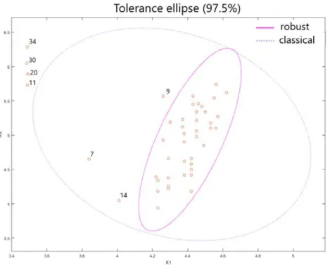
Figure 2.1 shows an example of the difference between considering robust and non-robust Mahalanobis distance to detect outliers. The observations are from the Hertzsprung-Russell Diagram of the Star Cluster CYG OB1 (Leroy and Rousseeuw

[1987]). It contains 47 stars data. In the figure, there are the 97.5% tolerance ellipses corresponding to the classical and a robust Mahalanobis distance. It is obvious how the presence of outliers influences the ellipsoid corresponding to the threshold for the classical Mahalanobis distance, masking the outliers 7, 9 and 14. Meanwhile, the robust distance correctly detects the atypical observations.

Figure 2.1: Star data with 97.5% tolerance ellipses corresponding to MD and RMD.

The procedure to find the MCD estimates required naive subsampling for min-imizing the objective function, but an improvement much more effective, the Fast-MCD, was introduced byRousseeuw and Driessen [1999] and the code is available in Matlab (Verboven and Hubert [2005]). Unfortunately, Fast-MCD still requires substantial running times for large dimension𝑝, because the number of candidate so-lutions grows exponentially with the dimension of the sample and, as a consequence, the procedure becomes computationally expensive for even moderately sized prob-lems.

(29)

Chapter 2. Robust outlier detection 29

2.2

Adjusted Minimum Covariance Determinant

(Adj MCD)

For the RMD based on MCD estimators, the classical quantile𝜒2

𝑝;0.975 is often used as the threshold to detect outliers. The problem is that fixing this threshold value is rather subjective in the robust distance case because there is no demonstration of the true distribution of the squared robust Mahalanobis distance. Furthermore, there is no reason why this fixed threshold should be appropriate for every data-set. The cut-off value should be adjusted to the sample size (Reimann et al. [2005]). On the other hand, if the data is clean and the observations come from a single mul-tivariate Normal distribution, there are no outliers, no observations coming from a different distribution, there are only extremes. In this case, the threshold should be infinity.

Since the squared RMD does not necessarily follow a chi-squared distribution, the problem of the selection of the cut-off value continues to be of crucial impor-tance, because there is no consensus. Filzmoser et al. [2005] proposed to use an adjusted quantile, instead of the classical choice. The adjusted threshold is esti-mated adaptively from the data, but their proposal is defined for a specific robust Mahalanobis distance, the one based on the MCD estimator.

The idea was based on measuring the difference between the empirical distri-bution of the squared robust distances and the distridistri-bution considered in theory, the chi-squared. Consider a sample {x1, ...,x𝑛} of dimension 𝑝. Let 𝐺(𝑢) be the distribution function of𝜒2

𝑝 and let 𝐺𝑛(𝑢) denote the empirical distribution function of the squared robust Mahalanobis distance 𝑅𝑀 𝐷𝑀 𝐶𝐷(x𝑖) from Equation 2.1.

For multivariate normally distributed samples, 𝐺𝑛 converges to 𝐺. Therefore, the next step is to compare the tails of 𝐺𝑛 and 𝐺 in order to detect outliers. The maximum possible positive difference between the two distributions is defined as 𝑝𝑛(𝛿), where 𝛿 =𝜒2𝑝;0.98 is the quantile that define the tails. In case of clean multi-variate normally distributed background data, the threshold should be infinity and no observation should be declared as an outlier. In this case, observations with a large RMD should be seen as extremes of the distribution. Therefore, it is necessary to consider a critical value𝑝𝑐𝑟𝑖𝑡, which will help to distinguish between outliers and extremes, if the departure in the tails between 𝐺𝑛 and 𝐺 is higher enough. The author derived the equation for the critical value 𝑝𝑐𝑟𝑖𝑡 by simulations and defined a measure of outliers in the sample as:

𝛼𝑛(𝛿) =

{︂

0, if 𝑝𝑛(𝛿)≤𝑝𝑐𝑟𝑖𝑡 𝑝𝑛(𝛿), if 𝑝𝑛(𝛿)> 𝑝𝑐𝑟𝑖𝑡

.

Then, in case of no contamination, i.e., no outliers, the maximum difference between the empirical and the distribution considered in theory, the chi-squared, should not be greater than the 𝑝𝑐𝑟𝑖𝑡 value. On the other hand, when the difference (in the tail) between the two distributions is big enough (greater than the𝑝𝑐𝑟𝑖𝑡value), then the𝑝𝑛(𝛿) should be selected as the𝛼 value for calculating the threshold𝑐𝑛(𝛿), which is determined as:

(30)

𝑐𝑛(𝛿) = 𝐺−𝑛1(1−𝛼𝑛(𝛿)). (2.2) Let us call this method Adj MCD. The idea of Filzmoser is an improved manner of estimating the threshold adaptively from the data. This procedure can be applied to any robust distance, other than the robust Mahalanobis distance based on the MCD estimator, the one used by Filzmoser. The only difference is to properly estimate the equations for the𝑝𝑐𝑟𝑖𝑡value based on the distance measure selected. The advantage is that the cut-off is adaptively estimated from the data and it improves the false positive rates, while maintaining the same true positive rates, except in some cases where the true positive rates can also be slightly declining.

2.3

Kurtosis

Another approach is the one proposed byPe˜na and Prieto[2001] andPe˜na and Prieto

[2007], which is based on the idea that high or low values of the kurtosis coefficient suggest the presence of outliers. The authors take the projections of the sample points onto the set of directions obtained by maximizing and minimizing the Kurtosis coefficient, and they also consider a set of random directions generated by a stratified sampling scheme. The authors proposed to project the “𝑛” cloud of points in_R𝑝 _over two new 𝑝−dimensional spaces: the first one obtained with the maximum kurtosis orthogonal direction, and the second one with the minimum kurtosis orthogonal direction, and also over a set of random directions. After obtaining the whole set of directions, the next step is to determine a “measure of outlyingness” for each observation (actually for their univariate projections𝑧_𝑖(𝑗)) as:

𝑟𝑖 =𝑚𝑎𝑥1≤𝑗≤𝑑

|𝑧_𝑖(𝑗)−𝑚𝑒𝑑𝑖𝑎𝑛(z(𝑗)₎_| 𝑀 𝐴𝐷(z(𝑗)₎ ,

where 𝑑 is the total number of directions in which the data are projected, the univariate projections are z(𝑗) _{= (}_𝑧(𝑗)

1 , ..., 𝑧 (𝑗)

𝑛 ),𝑚𝑒𝑑𝑖𝑎𝑛 is the univariate median and 𝑀 𝐴𝐷denotes the Median Absolute Deviation (Gauss[1816],Rousseeuw and Croux

[1993],Leys et al.[2013]), which is a robust measure of the variability of a univariate sample and it is defined as the median of the absolute deviations from the data’s median: 𝑀 𝐴𝐷(z(𝑗)) =𝑚𝑒𝑑𝑖𝑎𝑛(︁ ⃒⃒ ⃒𝑧 (𝑗) 𝑖 −𝑚𝑒𝑑𝑖𝑎𝑛(z (𝑗)₎⃒⃒ ⃒ )︁ .

With the above measure𝑟𝑖, a given observation is considered as an outlier if the condition 𝑟𝑖 being greater than a certain cut-off value holds. If the condition holds for some𝑖, a new sample composed of all observations whose𝑟𝑖 is less than the cut-off value is formed, and the procedure is applied again to the reduced sample. This is repeated until either no additional observations satisfy that their𝑟𝑖 is greater than the cut-off value, or the number of remaining observations is less than⌊(𝑛+𝑝+1)/2⌋. Finally, a Mahalanobis distance is computed for all observations labeled as outliers in the preceding steps, using the mean and the covariance estimator based upon the remaining observations. Let 𝑈 be the set of observations not labeled as outliers by the method, then the estimates of location ^𝜇_𝐾 and covariance matrix ^Σ𝐾 (where the

(31)

Chapter 2. Robust outlier detection 31

subscript 𝐾 stands as a notation for “Kurtosis”), based upon this subset 𝑈 defines a robust Mahalanobis distance as:

𝑅𝑀 𝐷𝐾(x𝑖) = (︁ (x𝑖−𝜇^𝐾) ^Σ −1 𝐾 (x𝑖−𝜇^𝐾) 𝑡)︁1/2 .

The final step is using this Mahalanobis distance to recover observations “mis-labeled” as outliers, i.e., if the observation𝑖 /∈𝑈 has 𝑅𝑀 𝐷𝐾(x𝑖)< 𝜒2𝑝;0.99, then x𝑖 is included in𝑈. The process is repeated until no more such observations are found or𝑈 becomes the set of all observations.

This method is a powerful approach for robust estimation and outlier detection. However, when the dimension 𝑝 of the sample space increases, the method wors-ens its performance, and in the presence of correlation between the variables, the method loses power (Marcano and Fermin [2013]). On the other hand, it is not very efficient computationally because of the optimization problem associated with the computation of the directions.

2.4

Orthogonalized Gnanadesikan-Kettenring (OGK)

Maronna and Zamar [2002] proposed the Orthogonalized Gnanadesikan-Kettenring (OGK) estimator. It was the result of applying a general method to a pairwise robust scatter matrix that may be non-positive definite, in order to obtain a positive-definite matrix. The method was applied to the robust covariance estimator from

Gnanadesikan and Kettenring[1972], which calculated a robust covariance estimate for two variables𝑋 and 𝑌 based on the following identity.

𝑐𝑜𝑣(𝑋, 𝑌) = 1 4

(︀

𝜎(𝑋+𝑌)2−𝜎(𝑋−𝑌)2)︀ .

where 𝜎 is a robust estimate of the standard deviation. The drawback is that these pairwise estimates will not necessarily be positive definite. So, Maronna and Zamar [2002] propose an eigen-decomposition based procedure to obtain positive-definiteness. The variables in an eigenvector space are orthogonal, which means the covariances are zero and it is sufficient to obtain robust variance estimates of the data projected onto each eigenvector direction. In OGK procedure, the eigenvalues are replaced with these robust variances, and the eigenvector transformation is applied in reverse to yield a positive semi-definite robust covariance matrix. OGK estimate is scale invariant of the original data matrix is robustly scaled, i.e., each component is divided by its robust variance. The authors stated that the procedure could be iterated, although it is not always better. They also find that using weighted estimates may improve the performance, in which case the observations are weighted according to their robust distances:

𝑅𝑀 𝐷𝑂𝐺𝐾(x𝑖) = (︁ (x𝑖−𝜇^𝑂𝐺𝐾) ^Σ −1 𝑂𝐺𝐾(x𝑖−𝜇^𝑂𝐺𝐾) 𝑡)︁1/2 ,

with ^𝜇_𝑂𝐺𝐾 and ^Σ𝑂𝐺𝐾 the robust OGK estimates. They use hard rejection weights, of the form 𝐼(𝑅𝑀 𝐷𝑂𝐺𝐾 < 𝑐), where 𝐼(·) is the indicator function and 𝑐 is the threshold value, which results from:

(32)

𝑐= 𝜒 2 𝑝;𝛽 𝑚𝑒𝑑(𝑅𝑀 𝐷𝑂𝐺𝐾1, ..., 𝑅𝑀 𝐷𝑂𝐺𝐾𝑛) 𝜒2 𝑝;0.5 , where 𝑚𝑒𝑑 denotes the median, and 𝜒2

𝑝;𝛽 is the 𝛽-quantile of the 𝜒2𝑝 distribution. The observations have full weight unless their robust distance is greater than 𝑐, in which case they will have zero weight.

2.5

Comedian

Sajesh and Srinivasan [2012] proposed a method, called the Comedian method to detect outliers from multivariate data based on thecomedian matrix estimator from

Falk [1997], which is also a robust estimate of scatter but it can be non-positive semi-definite. With the Comedian method, a positive definite scatter matrix can be obtained. The idea is based on the concept of comedian between two random variables𝑋 and 𝑌, which is defined as:

𝐶𝑂𝑀(𝑋, 𝑌) = 𝑚𝑒𝑑((𝑋−𝑚𝑒𝑑(𝑋))(𝑌 −𝑚𝑒𝑑(𝑌))). (2.3) The comedian is a robust measure of dependence between 𝑋 and 𝑌. Based on the median concept as a robust measure of location, there is a robust measure of dispersion for a random variable𝑋, which is theMedian Absolute Deviation (MAD) from the data’s median:

𝑀 𝐴𝐷(𝑋) = 𝑚𝑒𝑑𝑖𝑎𝑛(|𝑋−𝑚𝑒𝑑𝑖𝑎𝑛(𝑋)|).

A comedian matrix can be defined based on a multivariate version of (2.3). Let x = {x1, ...,x𝑝} be the 𝑛×𝑝 data matrix with 𝑛 being the sample size and 𝑝 the number of variables. Then the comedian matrix is defined as:

𝐶𝑂𝑀(x) = ( 𝐶𝑂𝑀(x𝑗,x𝑡) ) 𝑗, 𝑡= 1, ..., 𝑝 . (2.4)

Sajesh and Srinivasan [2012] also defined the correlation median matrix, based on the comedian matrix:

𝛿(𝑋) = 𝐷𝐶𝑂𝑀(𝑋)𝐷𝑡,

where 𝐷 is a diagonal matrix with diagonal elements 1/𝑀 𝐴𝐷(x𝑖), 𝑖 = 1, ..., 𝑝. Then, they adopted some transformations based on the eigenspace of the correlation median matrix and projections of the data, to overcome the non-positive semi-definiteness of the comedian matrix and to obtain robust estimates for location

^

𝜇_𝐶𝑂𝑀 and scatter ^Σ𝐶𝑂𝑀. The authors claim that the estimates can be improved through an iterative process, by replacing in the first step𝛿 by the estimated ^Σ𝐶𝑂𝑀 and repeat the other steps. For the outlier detection problem, a robust Mahalanobis distance can be defined.

𝑅𝑀 𝐷𝐶𝑂𝑀(x𝑖) =

(︁

(x𝑖 −𝜇^_𝐶𝑂𝑀) ^Σ_𝐶𝑂𝑀−1 (x𝑖−𝜇^_𝐶𝑂𝑀)𝑡 )︁1/2

. They defined the threshold value to detect outliers as

(33)

Chapter 2. Robust outlier detection 33 𝑐= 1.4826 𝜒 2 𝑝;0.95 𝑚𝑒𝑑(𝑅𝑀 𝐷𝐶𝑂𝑀1, ..., 𝑅𝑀 𝐷𝐶𝑂𝑀𝑛) 𝜒2 𝑝;0.5 .

Then, if any 𝑅𝑀 𝐷𝐶𝑂𝑀(x𝑖) > 𝑐, the corresponding observation x𝑖 is labeled as an outlier. By using this cut-off value and the robust Mahalanobis distance, a weight function can be defined and robust estimates for location and scatter can be obtained. The authors proved that these estimates are positive definite and approximately affine equivariant. They also study the breakdown value through simulations and the method showed good performance. Another conclusion of their work was that the efficiency of the method increases with the increase in dimension 𝑝, as examined through various numerical studies.

2.6

Summary

Through this chapter, a review of some of the most used robust estimators of loca-tion and covariance matrix is done. Rousseeuw[1985] proposed the MCD estimator which has good properties but becomes computationally expensive for even mod-erately sized problems. On the other hand, Filzmoser et al. [2005] proposed to use an adjusted quantile for this particular RMD definition (Adj MCD), estimated adaptively from the data. In general, the advantages over MCD with classical quan-tile, are that it holds the same properties but the false positive rate gets decreased, especially when there are no outliers in the data-set and the observations are gen-erated from a Normal distribution. Pe˜na and Prieto [2001] and Pe˜na and Prieto

[2007] proposed the Kurtosis approach based on the idea that maximizing and min-imizing the kurtosis coefficient is an indicator of the presence of outliers. It is a powerful procedure for robust estimation and outlier detection. However, it has some drawbacks when the dimension 𝑝 of the sample space grows, it is not very efficient computationally and in the presence of correlation between the variables, the method loses power. Maronna and Zamar[2002] proposed the OGK estimator, applying a general method to the pairwise robust scatter matrix fromGnanadesikan and Kettenring [1972]. With this procedure, a positive-definite scatter matrix can be obtained, which is of great importance when it is used in the Mahalanobis dis-tance since inversion of the covariance matrix is done. Sajesh and Srinivasan [2012] proposed the Comedian method (COM) to detect outliers from multivariate data based on the comedian matrix estimator fromFalk [1997]. Stated by their authors, OGK and Comedian method seems to have good performance for high dimension and good properties like high efficiency and approximate affine equivariance.

(34)

(35)

CHAPTER

3

Robust outlier detection based on shrinkage

In this section, a collection of RMD’s is proposed for outlier detection, especially in high dimension. They are based on considering different combinations of robust estimators of location and covariance matrix. Two basic options are considered for the location parameter: a component-wise median and the 𝐿1 multivariate median (Gower [1974], Brown [1983], Dodge [1987], Small [1990]). The notion of shrinkage (Ledoit and Wolf[2003a],Ledoit and Wolf[2003b],Ledoit and Wolf[2004],DeMiguel et al. [2013]) described in Chapter 1, is considered. Recall the shrinkage definition, from Equation1.4, which is based on the fact that shrinking a sample estimator to-wards a target estimator would help to reduce the estimation error. The shrinkage can be applied to both location and dispersion estimates, obtaining different combi-nations to define robust Mahalanobis distances. In the case of covariance matrices, the shrinkage provides positive definite and well-conditioned estimates, which is an additional advantage when the matrix needs to be inverted in the definition of an RMD. As for the covariance matrix, the proposed estimates consists on a shrink-age estimator over special cases of comedian matrices (Hall and Welsh [1985],Falk

[1997]), as the sample estimator to base the shrinking on. The comedian matrix is a robust estimator of scatter, and its definition is stated in Equation2.4, Section 2.5, Chapter 2, where it is also described in terms of its properties. The special cases of comedian matrices that are proposed are based upon a location parameter, which will be estimated using the robust estimator of centrality (or its shrinkage), in a way that an RMD can be obtained with meaningful combinations of both location and covariance matrix estimators. In this chapter, we analyze the best option for shrinking the location and the scale. Through a simulation study, the satisfactory practical performance is shown, especially when the dimension of the problem grows. The computational cost is studied by both simulations and a real data-set example.

3.1

Location parameter

Letx={x1, ...,x𝑝}be the𝑛×𝑝data matrix with𝑛being the sample size and𝑝the number of variables. Based on the fact that the 𝑚𝑒𝑑𝑖𝑎𝑛 is a better choice in terms

(36)

of robustness, we start by considering as a location estimator the component-wise median:

^

𝜇_𝐶𝐶𝑀 = (𝑚𝑒𝑑𝑖𝑎𝑛(x1), ..., 𝑚𝑒𝑑𝑖𝑎𝑛(x𝑝)), (3.1) where 𝑚𝑒𝑑𝑖𝑎𝑛 denotes the univariate median and (x𝑗) = (𝑥1𝑗, ..., 𝑥𝑛𝑗)𝑇 for all 𝑗 = 1, ..., 𝑝 is the 𝑗-th column of x.

Another option is to consider a multivariate median ^𝜇_{𝑀 𝑀} called 𝐿1−median which is a robust and highly efficient estimator of central tendency (Lopuhaa and Rousseeuw[1991], Vardi and Zhang[2002], Hubert [2011]). It is defined as:

^ 𝜇_{𝑀 𝑀} =𝑎𝑟𝑔𝑚𝑖𝑛x𝑚, 𝑚∈{1,...,𝑛} 1 𝑛 𝑛 ∑︁ 𝑖=1 ||x𝑚−x𝑖||1. (3.2)

DeMiguel et al. [2013] proposed a shrinkage estimator over the sample mean, towards a scaled vector of ones as the target. In the same way we propose to study shrinkage estimators for both (3.1) and (3.2). Consider𝜈𝜇eas the target estimator, where e is the 𝑝−dimensional vector of ones, and consider ^𝜇_𝐶𝐶𝑀 as the sample estimator ^𝐸. Then, the shrinkage estimator over the component-wise median is:

^

𝜇_𝑆ℎ₍_𝐶𝐶𝑀₎= (1−𝜂) ^𝜇_𝐶𝐶𝑀 +𝜂𝜈𝜇e.

The scaling factor𝜈𝜇and the intensity𝜂should minimize the expected quadratic loss, that is:

min𝜈𝜇,𝜂 𝐸 [︁ ⃦ ⃦𝜇^_𝑆ℎ₍_𝐶𝐶𝑀₎−𝜇 ⃦ ⃦ 2 2 ]︁ s.t. 𝜇^_𝑆ℎ₍_𝐶𝐶𝑀₎ = (1−𝜂)𝜇^_𝐶𝐶𝑀 +𝜂𝜈𝜇e, (3.3) where‖x‖2₂ =∑︀𝑝 𝑗=1𝑥 2 𝑗.

Proposition 1 The solution of the problem in (3.3) is:

^ 𝜈𝜇= ^ 𝜇_𝐶𝐶𝑀e 𝑝 , 𝜂^= 𝐸[︀ ‖𝜇^_𝐶𝐶𝑀 −𝜇‖2₂]︀ 𝐸[︀‖𝜇^_𝐶𝐶𝑀 −𝜈^𝜇e‖2₂ ]︀. (3.4)

See the proof in Appendix A.1. Note that the denominator in the above ex-pression (3.4) is estimable, but the numerator is not straightforward because 𝜇 is unknown. Then, it is necessary to provide another expression for the numerator.

Chu [1955] investigated the distribution for the sample median estimator and ob-tained the following result about the variance in presence of normality. Fix 𝑗, for 𝑗 ∈ {1, ..., 𝑝}: 𝜎_𝜇2_^ 𝐶𝐶𝑀 𝑗 =𝑉 𝑎𝑟(𝜇^𝐶𝐶𝑀 𝑗) = 𝜋 2𝑛𝜎 2 xj.

Therefore, the numerator in the expression (3.4) for determining the ^𝜂in Propo-sition1 is:

(37)

Chapter 3. Robust outlier detection based on shrinkage 37 𝐸[︀‖𝜇^_𝐶𝐶𝑀 −𝜇‖2₂]︀ =𝐸 [︃ _𝑝 ∑︁ 𝑗=1 (𝜇^_{𝐶𝐶𝑀 𝑗} −𝜇_𝑗)2 ]︃ = 𝑝 ∑︁ 𝑗=1 𝜎_𝜇2_^ 𝐶𝐶𝑀 𝑗 = 𝜋 2𝑛 𝑝 ∑︁ 𝑗=1 𝜎_x2_𝑗. (3.5) We need to estimate 𝜎2

x𝑗 robustly, and we will do so as explained in the next

Section 3.2, with property (3.10). The estimate for ^𝜂 in expression (3.4) can be calculated as stated in Equation3.11 in next Section 3.2.

On the other hand, consider 𝜈𝜇e again as the target estimator and consider ^

𝜇_{𝑀 𝑀} as the sample estimator. Then, the shrinkage estimator over the multivariate 𝐿1−median is:

^

𝜇_𝑆ℎ₍_{𝑀 𝑀}₎= (1−𝜂) ^𝜇_{𝑀 𝑀} +𝜂𝜈𝜇e.

The scaling factor𝜈𝜇and the intensity𝜂should minimize the expected quadratic loss: min𝜈𝜇,𝜂 𝐸 [︁ ⃦ ⃦𝜇^_𝑆ℎ₍_{𝑀 𝑀}₎−𝜇 ⃦ ⃦ 2 2 ]︁ s.t. 𝜇^_𝑆ℎ₍_{𝑀 𝑀}₎ = (1−𝜂)𝜇^_{𝑀 𝑀} +𝜂𝜈𝜇e, (3.6) where‖x‖2₂ =∑︀𝑝 𝑗=1𝑥 2 𝑗.

Proposition 2 The solution of the problem in (3.6) is:

^ 𝜈𝜇 = ^ 𝜇_{𝑀 𝑀}e 𝑝 , 𝜂^= 𝐸[︀‖𝜇^_{𝑀 𝑀}−𝜇‖2]︀ 𝐸[︀ ‖𝜇^_{𝑀 𝑀} −𝜈^𝜇e‖2 ]︀ . (3.7)

The proof is Appendix A.2. As in the previous case, the denominator in the 𝜂 expression (3.7) can be described as:

𝐸[︀ ‖𝜇^_{𝑀 𝑀}−𝜇‖2₂]︀ =𝐸 [︃ 𝑝 ∑︁ 𝑗=1 (𝜇^_{𝑀 𝑀 𝑗}−𝜇_𝑗)2 ]︃ = 𝑝 ∑︁ 𝑗=1 𝜎_𝜇2_^ 𝑀 𝑀 𝑗 .

Bose and Chaudhuri [1993], Bose [1995] and M¨ott¨onen et al. [2010] investi-gated the asymptotic distribution for the𝐿1−median. In page 184, section 3, from

M¨ott¨onen et al. [2010], the authors describe the necessity of the following two as-sumptions, for x a 𝑝−variate random vector with cdf 𝐹, density function 𝑓 and 𝑝 >1:

(C1) The 𝑝−variate density function of xis continuous and bounded.

(38)

According to Theorem 2, page 185, section 3 in M¨ott¨onen et al. [2010], under assumptions C1 and C2,√𝑛𝜇^_{𝑀 𝑀} →𝑑𝑁𝑝(0, 𝐴−1𝐵𝐴−1), where ^𝜇𝑀 𝑀 is the observed spatial median, and 𝐴 and 𝐵 are the following:

𝐴(x) = 1 ||x|| [︂ 𝐼𝑝− xx𝑡 ||x||2 ]︂ 𝐵(x) = xx 𝑡 ||x||2 .

In section 4, page 185 from M¨ott¨onen et al. [2010], the authors also provide an estimation for the asymptotic covariance matrix 𝐴−1_𝐵𝐴−1 _{of the spatial median.} They are assuming the true value ^𝜇_{𝑀 𝑀} =0 is zero (condition C2). Then they write

^

𝐴=𝑎𝑣𝑒{𝐴(x𝑖−𝜇^𝑀 𝑀)}and ^𝐵 =𝑎𝑣𝑒{𝐵(x𝑖−𝜇^𝑀 𝑀)} and prove that under C1 and C2: ^𝐴→𝑃 𝐴and ^𝐵 →𝑃 𝐵, which means that the estimators converge in probability to the population values 𝐴 and 𝐵, respectively. This result is Theorem 3, section 4, page 185 from M¨ott¨onen et al. [2010]. According to the authors (stated in page 186), Theorems 2 and 3 suggest that the distribution of ^𝜇_{𝑀 𝑀} can be approximated by 𝑁𝑝 (︁ 𝜇,_𝑛1𝐴^−1𝐵^𝐴^−1 )︁ , where ^𝐴(x𝑖) = _||_x1 𝑖||2 (︁ 𝐼𝑝− x𝑖x𝑡𝑖 ||x𝑖||22 )︁ and ^𝐵(x𝑖) = x𝑖x𝑡𝑖 ||x𝑖||22, with x𝑖 ∈R𝑝, for each 𝑖= 1, ..., 𝑛.

The asymptotic result is also given in page 9-11 ofBecker et al.[2014] as well as the estimate for the approximate covariance matrix on page 11. The assumptions in that paper are analogous, but it can be seen that C2 assumption about the spatial median being zero is not necessary, only that it is unique and the density function 𝑓 is bounded and continuous at 𝜇 (Section 1.4, page 9 from Becker et al. [2014]). The difference is that when approximating the covariance matrix, the data should be centered around the estimated spatial median.

The numerator𝐸[︀‖𝜇^_{𝑀 𝑀} −𝜇‖2]︀

from the expression (3.7) can be approximated with𝑡𝑟𝑎𝑐𝑒(︁_𝑛1𝐴^−1_𝐵_^_𝐴_^−1)︁_{, as suggested by} _M¨_ott¨_{onen et al.} _[₂₀₁₀_{]. Then the} estima-tors for ^𝜈 and ^𝜂 in Equation 3.7 would be estimated as:

^ 𝜈𝜇 = ^ 𝜇_{𝑀 𝑀}e 𝑝 and 𝜂^= 𝑡𝑟𝑎𝑐𝑒 (︁ 1 𝑛𝐴^ −1_𝐵_^_𝐴_^−1)︁ ‖𝜇^_{𝑀 𝑀} −𝜈^𝜇e‖ 2 .

3.2

Dispersion parameter

Based on the median concept, which is a robust measure of location, there is a robust measure of dispersion for a random variable𝑋, which is theMedian Absolute Deviation (MAD) from the data’s median:

𝑀 𝐴𝐷(𝑋) = 𝑚𝑒𝑑𝑖𝑎𝑛(|𝑋−𝑚𝑒𝑑𝑖𝑎𝑛(𝑋)|).

Falk[1997] showed the following relation, assuming normality, between the𝑀 𝐴𝐷 and the standard deviation 𝜎𝑋:

𝑀 𝐴𝐷(𝑋) = 𝜎𝑋Φ−1(3/4), (3.8) where Φ denotes the standard normal cdf. Taking the square in (3.8) we obtain a relation between the variance 𝜎2_𝑋 and 𝑀 𝐴𝐷2(𝑋):

(39)

Chapter 3. Robust outlier detection based on shrinkage 39

𝜎_𝑋2 = 2.198·𝑀 𝐴𝐷2(𝑋).

Extending the idea of the 𝑀 𝐴𝐷, a robust measure of dependence between two random variables 𝑋 and 𝑌 is the comedian (Falk [1997]):

𝐶𝑂𝑀(𝑋, 𝑌) = 𝑚𝑒𝑑((𝑋−𝑚𝑒𝑑(𝑋)) (𝑌 −𝑚𝑒𝑑(𝑌))) . (3.9) The comedian generalizes the MAD because 𝐶𝑂𝑀(𝑋, 𝑋) = 𝑀 𝐴𝐷2₍_𝑋_{), and} also has the highest possible breakdown point (Falk [1997]). An important fact is that the comedian parallels the covariance, but the latter requires the existence of the first two moments of the two random variables, whereas the comedian always exists. Other known properties of the comedian are that it is symmetric, location invariant and scale equivariant. Furthermore, Hall and Welsh [1985] discussed the strong consistency and asymptotic normality of the MAD, and Falk [1997] estab-lished similar results for the comedian.

Finally, let us recall that a comedian matrix can be defined based on a multi-variate version of (3.9). Let x={x1, ...,x𝑝}be the 𝑛×𝑝 data matrix with 𝑛 being the sample size and𝑝the number of variables. Then the comedian matrix is defined as:

𝐶𝑂𝑀(x) = (𝐶𝑂𝑀(x𝑗,x𝑡)), 𝑗, 𝑡= 1, ..., 𝑝 .

Note that from relation described in (3.8), one can consider the adjusted come-dian:

^

𝑆𝐶𝐶𝑀 = 2.198·𝐶𝑂𝑀(x).

Recall the previous Section3.1in which we needed to provide a robust estimator for 𝜎2

x𝑗, for each 𝑗 = 1, ..., 𝑝 (Equation 3.5) note that, because of the relation in

(3.8): 𝑡𝑟𝑎𝑐𝑒( ^𝑆𝐶𝐶𝑀) = 𝑝 ∑︁ 𝑗=1 2.198·𝐶𝑂𝑀(x𝑗,x𝑗) = 𝑝 ∑︁ 𝑗=1 2.198·𝑀 𝐴𝐷2(x𝑗) = 𝑝 ∑︁ 𝑗=1 𝜎_x2 𝑗. (3.10)

Thus, when considering a shrinkage estimator of the component-wise median, in order to estimate the variance of 𝜇^_𝐶𝐶𝑀 needed in the expression (3.4) for the shrinkage intensity ^𝜂, and according to the relation (3.5), we propose to estimate ∑︀𝑝

𝑗=1𝜎 2

x𝑗 using the𝑡𝑟𝑎𝑐𝑒( ^𝑆𝐶𝐶𝑀). Therefore, the estimates for ^𝜈𝜇and ^𝜂in expression

(3.4) can be calculated as:

^ 𝜈𝜇 = ^ 𝜇_𝐶𝐶𝑀e 𝑝 and 𝜂^= (𝜋/2𝑛)𝑡𝑟𝑎𝑐𝑒( ^𝑆𝐶𝐶𝑀) ‖𝜇^_𝐶𝐶𝑀 −𝜈^𝜇e‖2₂ . (3.11)

Note that ^𝑆𝐶𝐶𝑀 is a robust alternative for the covariance matrix, but in general, it is not positive (semi-) definite (see Falk [1997]). Since we need this property for

(40)

inverting the covariance matrix in a Mahalanobis distance, we propose a shrinkage over ^𝑆𝐶𝐶𝑀, because of its advantage of always providing a positive definite and well-conditioned matrix. Therefore, if a shrinkage estimator is considered for the dispersion parameter:

^

Σ𝑆ℎ= (1−𝜂) ^𝐸+𝜂𝑇 ,^ (3.12) we propose to use in (3.12), the estimator ^𝐸 = ^𝑆𝐶𝐶𝑀.

Several choices for the shrinkage target ^𝑇 have been proposed in the literature. For example, Ledoit and Wolf [2003b] proposed a weighted average of the sample covariance matrix and a single-index covariance matrix. Ledoit and Wolf [2003a] proposed selecting the shrinkage target as a “constant correlation matrix”, whose correlations are set equal to the average of all sample correlations. Finally, Ledoit and Wolf [2004] proposed to use a multiple of the identity matrix as the shrink-age target. The authors proved that the resulting shrinkshrink-age covariance matrix is well-conditioned, even if the sample covariance matrix is not. There is also another approach introduced by DeMiguel et al. [2013]. The authors proposed a shrinkage estimator both for the covariance matrix and its inverse. The estimators were con-structed as a convex combination of the sample covariance matrix or its inverse, respectively, and a scaled shrinkage target, which they consider the scaled identity matrix asLedoit and Wolf [2004]. Therefore, we propose to use as shrinkage target

^

𝑇 =𝜈Σ𝐼. Thus (3.12) results in:

^

Σ𝑆ℎ(𝐶𝐶𝑀)= (1−𝜂) ^𝑆𝐶𝐶𝑀 +𝜂𝜈Σ𝐼 .

Finally, the scaling parameter 𝜈Σ and the shrinkage intensity parameter𝜂 needs to be estimated. They both are chose