mclust 5: Clustering, Classification and Density Estimation Using Gaussian Finite Mixture Models

(1)

mclust 5: Clustering, Classification and

Density Estimation Using Gaussian Finite

Mixture Models

by Luca Scrucca, Michael Fop, T. Brendan Murphy and Adrian E. Raftery

Abstract Finite mixture models are being used increasingly to model a wide variety of random phenomena for clustering, classification and density estimation.mclustis a powerful and popular package which allows modelling of data as a Gaussian finite mixture with different covariance structures and different numbers of mixture components, for a variety of purposes of analysis. Recently, version 5 of the package has been made available on CRAN. This updated version adds new covariance structures, dimension reduction capabilities for visualisation, model selection criteria, initialisation strategies for the EM algorithm, and bootstrap-based inference, making it a full-featured R package for data analysis via finite mixture modelling.

Introduction

mclust(Fraley et al.,2016) is a popular R package for model-based clustering, classification, and density estimation based on finite Gaussian mixture modelling. An integrated approach to finite mixture models is provided, with functions that combine model-based hierarchical clustering, EM for mixture estimation and several tools for model selection. Thusmclustprovides a comprehensive strategy for clustering, density estimation and discriminant analysis. A variety of covariance structures obtained through eigenvalue decomposition are available. Functions for performing single E and M steps and for simulating data for each available model are also included. Additional ways of displaying and visualising fitted models along with clustering, classification, and density estimation results are also provided. It has been used in a broad range of contexts including geochemistry (Templ et al.,2008;Ellefsen et al.,2014), chemometrics (Fraley and Raftery,2006a,2007b), DNA sequence analysis (Verbist et al.,2015), gene expression data (Yeung et al.,2001;Li et al.,2005;Fraley and Raftery,

2006b), hydrology (Kim et al.,2014), wind energy (Kazor and Hering,2015), industrial engineering (Campbell et al.,1999), epidemiology (Flynt and Daepp,2015), food science (Kozak and Scaman,

2008), clinical psychology (Suveg et al.,2014), political science (Ahlquist and Breunig,2012;Jang and Hitchcock,2012), and anthropology (Konigsberg et al.,2009).

One measure of the popularity of mclustis provided by the download logs of the RStudio

(http://www.rstudio.com) CRAN mirror (available athttp://cran-logs.rstudio.com). The

cran-logspackage (Csardi,2015) makes it easy to download such logs and graph the number of downloads

over time. We usedcranlogsto query the RStudio download database over the past three years. In

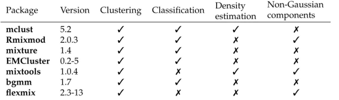
addition tomclust, other R packages which handle Gaussian finite mixture modelling as part of their capabilities have been included in the comparison:Rmixmod(Lebret et al.,2015),mixture(Browne et al.,2015),EMCluster(Chen and Maitra,2015),mixtools(Benaglia et al.,2009), andbgmm(Biecek et al.,2012). We also includedflexmix(Leisch,2004;Grün and Leisch,2007,2008) which provides a general framework for finite mixtures of regression models using the EM algorithm, since it can be adapted to perform Gaussian model-based clustering using a limited set of models (only the diagonal and unconstrained covariance matrix models). Table1summarises the functionalities of the selected packages.

Package Version Clustering Classification Density estimation Non-Gaussian components mclust 5.2 3 3 3 7 Rmixmod 2.0.3 3 3 7 3 mixture 1.4 3 3 7 7 EMCluster 0.2-5 3 3 7 7 mixtools 1.0.4 3 7 3 3 bgmm 1.7 3 3 7 7 flexmix 2.3-13 3 7 7 3

Table 1:Capabilities of the selected packages dealing with finite mixture models.

(2)

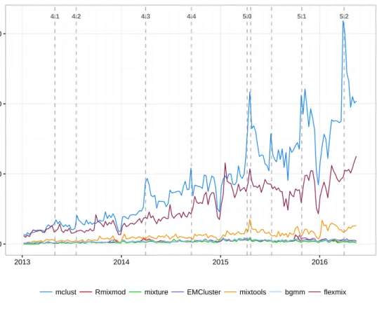
packages. The popularity ofmclusthas been increasing steadily over time with a first high peak around mid April 2015, probably due to the release of R version 3.2 and, shortly after, the release of version 5 ofmclust. Then, successive peaks occurred in conjunction with the release of package’s updates. Based on these logs,mclustis the most downloaded package dealing with Gaussian mixture

models, followed byflexmixwhich, as mentioned, is a more general package for fitting mixture

models but with limited clustering capabilities.

4.1 4.2 4.3 4.4 5.0 5.1 5.2 0 2000 4000 6000 2013 2014 2015 2016 Number of w eekly do wnloads

mclust Rmixmod mixture EMCluster mixtools bgmm flexmix

Figure 1:Number of weekly downloads from the RStudio CRAN mirror over time for some R packages dealing with Gaussian finite mixture modelling.

Another aspect that can be considered as a proxy for the popularity of a package is the mutual dependencies structure between R packages1_{. This can be represented as a graph with packages at the} vertices and dependencies (either “Depends”, “Imports”, “LinkingTo”, “Suggests” or “Enhances”) as directed edges, and analysed through thePageRankalgorithm used by the Google search engine (Brin and Page,1998). For the packages considered previously, we used thepage.rankfunction available in theigraphpackage (Csardi and Nepusz,2006) and we obtained the ranking reported in Table2, which approximately reproduces the results discussed above. Note thatmclustis among the top 100 packages on CRAN by this ranking. Finally, its popularity is also indicated by the 55 other CRAN packages listed as reverse dependencies, either “Depends”, “Imports” or “Suggests”.

mclust Rmixmod mixture EMCluster mixtools bgmm flexmix

75 2300 2319 2143 1698 3736 270

Table 2:Ranking obtained with thePageRankalgorithm for some R packages dealing with Gaussian finite mixture modelling. At the time of writing there are 8663 packages on CRAN.

Earlier versions of the package have been described inFraley and Raftery(1999),Fraley and Raftery(2003), andFraley et al.(2012). In this paper we discuss some of the new functionalities

available inmclustversion≥5. In particular we describe the newly available models, dimension

reduction for visualisation, bootstrap-based inference, implementation of different model selection criteria and initialisation strategies for the EM algorithm.

The reader should first install the latest version of the package from CRAN with

> install.packages("mclust")

(3)

Then the package is loaded into an R session using the command > library(mclust) __ ___________ __ _____________ / |/ / ____/ / / / / / ___/_ __/ / /|_/ / / / / / / / /\__ \ / / / / / / /___/ /___/ /_/ /___/ // / /_/ /_/\____/_____/\____//____//_/ version 5.2

Type 'citation("mclust")' for citing this R package in publications.

All the datasets used in the examples are available inmclustor in other R packages, such asgclus

(Hurley,2012),rrcov(Todorov and Filzmoser,2009) andtourr(Wickham et al.,2011), and can be installed from CRAN using the above procedure, except where noted differently.

Gaussian finite mixture modelling

Letx={x1,x2, . . . ,xi, . . . ,xn}be a sample ofnindependent identically distributed observations. The

distribution of every observation is specified by a probability density function through a finite mixture

model ofGcomponents, which takes the following form

f(xi;Ψ) = G

∑

k=1

πkfk(xi;θk), (1)

whereΨ={π₁, . . . ,πG−1,θ1, . . . ,θG}are the parameters of the mixture model, fk(xi;θk)is thekth

component density for observationxiwith parameter vectorθk,(π1, . . . ,πG−1)are the mixing weights

or probabilities (such thatπk>0,∑Gk=1πk=1), andGis the number of mixture components.

Assuming thatGis fixed, the mixture model parametersΨare usually unknown and must be

estimated. The log-likelihood function corresponding to equation (1) is given by`(Ψ;x1, . . . ,xn) =

∑n

i=1log(f(xi;Ψ)). Direct maximisation of the log-likelihood function is complicated, so the maximum

likelihood estimator (MLE) of a finite mixture model is usually obtained via the EM algorithm (Dempster et al.,1977;McLachlan and Peel,2000).

In the model-based approach to clustering, each component of a finite mixture density is usually associated with a group or cluster. Most applications assume that all component densities arise from the same parametric distribution family, although this need not be the case in general. A popular model is the Gaussian mixture model (GMM), which assumes a (multivariate) Gaussian distribution for each component, i.e. fk(x;θk) ∼N(µ_k,Σk). Thus, clusters are ellipsoidal, centered at the mean

vectorµ_k, and with other geometric features, such as volume, shape and orientation, determined by the covariance matrixΣk. Parsimonious parameterisations of the covariances matrices can be obtained

by means of an eigen-decomposition of the formΣk=λkDkAkD>k, whereλkis a scalar controlling

the volume of the ellipsoid,Akis a diagonal matrix specifying the shape of the density contours with

det(Ak) =1, andDkis an orthogonal matrix which determines the orientation of the corresponding

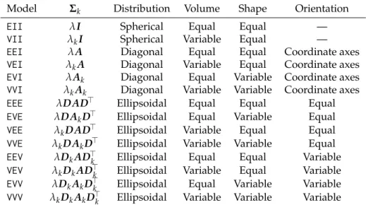
ellipsoid (Banfield and Raftery,1993;Celeux and Govaert,1995). In one dimension, there are just two models:Efor equal variance andVfor varying variance. In the multivariate setting, the volume, shape, and orientation of the covariances can be constrained to be equal or variable across groups. Thus, 14 possible models with different geometric characteristics can be specified. Table3reports all such models with the corresponding distribution structure type, volume, shape, orientation, and associated model names. In Figure2the geometric characteristics are shown graphically.

Starting with version 5.0 ofmclust, four additional models have been included: EVV, VEE, EVE, VVE. Models EVV and VEE are estimated using the methods described inCeleux and Govaert(1995),

and the estimation of models EVE and VVE is carried out using the approach discussed byBrowne

and McNicholas(2014). In the models VEE, EVE and VVE it is assumed that the mixture components share the same orientation matrix. This assumption allows for a parsimonious characterisation of the clusters, while still retaining flexibility in defining volume and shape.

Model-based clustering

To illustrate the new modelling capabilities ofmclustfor model-based clustering consider thewine

dataset contained in thegclusR package. This dataset provides 13 measurements obtained from a

chemical analysis of 178 wines grown in the same region in Italy but derived from three different cultivars (Barolo, Grignolino, Barbera).

(4)

Model Σk Distribution Volume Shape Orientation

EII

λI Spherical Equal Equal —

VII

λkI Spherical Variable Equal —

EEI

λA Diagonal Equal Equal Coordinate axes

VEI

λkA Diagonal Variable Equal Coordinate axes

EVI

λAk Diagonal Equal Variable Coordinate axes

VVI

λkAk Diagonal Variable Variable Coordinate axes

EEE

λDAD> Ellipsoidal Equal Equal Equal

EVE

λDAkD> Ellipsoidal Equal Variable Equal

VEE

λkDAD> Ellipsoidal Variable Equal Equal

VVE

λkDAkD> Ellipsoidal Variable Variable Equal

EEV

λDkAD>k Ellipsoidal Equal Equal Variable

VEV

λkDkAD>k Ellipsoidal Variable Equal Variable

EVV

λDkAkD>k Ellipsoidal Equal Variable Variable

VVV

λkDkAkD>k Ellipsoidal Variable Variable Variable

Table 3: Parameterisations of the within-group covariance matrixΣk for multidimensional data

available in themclustpackage, and the corresponding geometric characteristics.

EII VII EEI VEI EVI

VVI EEE EVE VEE EEV

VEV EVV VVE VVV

Figure 2:Ellipses of isodensity for each of the 14 Gaussian models obtained by eigen-decomposition in case of three groups in two dimensions.

> data(wine, package = "gclus")

> Class <- factor(wine$Class, levels = 1:3,

labels = c("Barolo", "Grignolino", "Barbera")) > X <- data.matrix(wine[,-1])

> mod <- Mclust(X) > summary(mod$BIC) Best BIC values:

EVE,3 VVE,3 VVE,6

BIC -6873.257 -6896.83693 -6906.37460

BIC diff 0.000 -23.57947 -33.11714

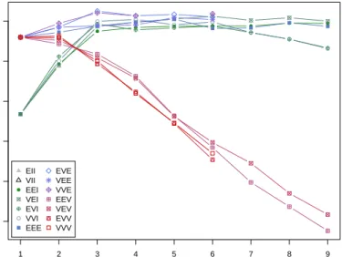
> plot(mod, what = "BIC", ylim = range(mod$BIC[,-(1:2)], na.rm = TRUE), legendArgs = list(x = "bottomleft"))

(5)

−9500 −9000 −8500 −8000 −7500 −7000 Number of components BIC ● ● ● ● ● ● ● ● ● ● ● ● ● ● ● ● ● ● ● ● ● ● ● ● ● ● ● ● ● ● ● ● ● ● ● ● 1 2 3 4 5 6 7 8 9 ● ● ● ● EII VII EEI VEI EVI VVI EEE EVE VEE VVE EEV VEV EVV VVV

Figure 3:BIC plot for models fitted to thewinedata.

components and the covariance parameterisation are selected using the Bayesian Information Criterion (BIC). A summary showing the top-three models and a plot of the BIC traces (see Figure3) for all the models considered is then obtained. In the last plot we adjusted the range of the y-axis so to remove those models with lower BIC values. There is a clear indication of a three-component mixture with covariances having different shapes but the same volume and orientation (EVE). Note that all the top three models are among the models added to the latest major release ofmclust.

A summary of the selected model is obtained as:

> summary(mod)

---Gaussian finite mixture model fitted by EM algorithm

---Mclust EVE (ellipsoidal, equal volume and orientation) model with 3 components:

log.likelihood n df BIC ICL

-3032.45 178 156 -6873.257 -6873.549 Clustering table:

1 2 3 63 51 64

The fitted model provides an accurate recovery of the true classes:

> table(Class, mod$classification) Class 1 2 3 Barolo 59 0 0 Grignolino 4 3 64 Barbera 0 48 0 > adjustedRandIndex(Class, mod$classification) [1] 0.8803998

The latter index is the adjusted Rand index (ARI;Hubert and Arabie,1985), which can be used for evaluating a clustering solution. The ARI is a measure of agreement between two partitions, one estimated by a statistical procedure independent of the labelling of the groups, and one being the true classification. It has zero expected value in the case of a random partition, and it is bounded above by 1, with higher values representing better partition accuracy.

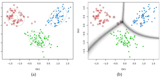
To visualise the clustering structure and the geometric characteristics induced by an estimated Gaussian finite mixture model we may project the data onto a suitable dimension reduction subspace.

The functionMclustDR()implements the methodology introduced inScrucca(2010). The estimated

directions which span the reduced subspace are defined as a set of linear combinations of the original features, ordered by importance as quantified by the associated eigenvalues. By default, information on the dimension reduction subspace is provided by both the variation on cluster means and, depending

(6)

on the estimated mixture model, on the variation on cluster covariances. This methodology has been extended to supervised classification byScrucca(2014). Furthermore, a tuning parameter has been included which enables the recovery of most of the separating directions, i.e. those that show maximal separation among groups. Other dimension reduction techniques for finding the directions of optimum separation have been discussed in detail byHennig(2004) and implemented in the package

fpc(Hennig,2015).

ApplyingMclustDRto the wine data example, such directions are obtained as follows:

> drmod <- MclustDR(mod, lambda = 1) > summary(drmod)

---Dimension reduction for model-based clustering and classification ---Mixture model type: Mclust (EVE, 3)

Clusters n 1 63 2 51 3 64

Estimated basis vectors:

Dir1 Dir2 Alcohol 0.11701058 0.2637302 Malic -0.02814821 0.0489447 Ash -0.18258917 0.5390056 Alcalinity -0.02969793 -0.0309028 Magnesium 0.00575692 0.0122642 Phenols -0.18497201 -0.0016806 Flavanoids 0.45479873 -0.2948947 Nonflavanoid 0.59278569 -0.5777586 Proanthocyanins 0.05347167 0.0508966 Intensity -0.08328239 0.0332611 Hue 0.42950365 -0.4588969 OD280 0.40563746 -0.0369229 Proline 0.00075867 0.0010457 Dir1 Dir2 Eigenvalues 1.5794 1.332 Cum. % 54.2499 100.000

By setting the optional tuning parameterlambda = 1, instead of the default value0.5, only the information on cluster means is used for estimating the directions. In this case, the dimension of the subspace isd=min(p,G−1), wherepis the number of variables andGthe number of mixture components or clusters. In the data example, there arep=13 features andG=3 clusters, so the

dimension of the reduced subspace isd = 2. As a result, the projected data show the maximal

separation among clusters, as shown in Figure4a, which is obtained with

> plot(drmod, what = "contour")

On the same subspace we can also plot the uncertainty boundaries corresponding to the MAP classification:

> plot(drmod, what = "boundaries", ngrid = 200)

and then add a circle around the misclassified observations

> miscl <- classError(Class, mod$classification)$misclassified > points(drmod$dir[miscl,], pch = 1, cex = 2)

Model selection

A central question in finite mixture modelling is how many components should be included in the mixture. In GMMs we need also to decide which covariance parameterisation to adopt. Both questions can be addressed by information criteria, such as the BIC (Schwartz,1978;Fraley and Raftery,1998)

(7)

−1.5 −1.0 −0.5 0.0 0.5 1.0 1.5 −1.5 −1.0 −0.5 0.0 0.5 1.0 Dir1 Dir2 0.5 1 1.5 0.5 1 1.5 0.5 1 1.5 ● ● ● ● ● ● ● ● ● ● ● ● ● ● ● ● ● ● ● ● ● ● ● ● ● ● ● ● ● ● ● ● ● ● ● ● ● ● ● ● ● ● ● ● ● ● ● ● ● ● ● ●● ● ● ● ● ● ● ● ● ● ● (a) −1.5 −1.0 −0.5 0.0 0.5 1.0 1.5 −1.5 −1.0 −0.5 0.0 0.5 1.0 Dir1 Dir2 ● ● ● ● ● ● ● ● ● ● ● ● ● ● ● ● ● ● ● ● ● ● ● ● ● ● ● ● ● ● ● ● ● ● ● ● ● ● ● ● ● ● ● ● ● ● ● ● ● ● ● ●● ● ● ● ● ● ● ● ● ● ● ● ● ● ● ● ● ● (b)

Figure 4: Contour plot of estimated mixture densities (a) and uncertainty boundaries (b) on the projection subspace estimated withMclustDRfor thewinedataset.

or the integrated complete-data likelihood criterion (ICL;Biernacki et al.,2000). The selection of the order of the mixture, i.e. the number of mixture components or clusters, can be also performed by formal hypothesis testing; for a recent review seeMcLachlan and Rathnayake(2014).

Information criteria are based on penalised forms of the log-likelihood. As the likelihood increases with the addition of more components, a penalty term for the number of estimated parameters is subtracted from the log-likelihood. The BIC is a popular choice in the context of GMMs, and takes the form

BICM,G=2`M,G(x|Ψb)−νlog(n),

where`_M_,_G(x|Ψb)is the log-likelihood at the MLEΨbfor modelMwithGcomponents,nis the sample

size, andνis the number of estimated parameters. The pair{M,G}which maximises BICM,Gis

selected. Given some necessary regularity conditions, BIC is derived as an approximation to the model evidence using the Laplace method. Although these conditions do not hold for mixture models in general (Aitkin and Rubin,1985), some consistency results apply (Roeder and Wasserman,1997;

Keribin,2000) and the criterion has been shown to perform well in applications (Fraley and Raftery,

1998).

In themclustpackage, BIC is used by default for model selection. The functionmclustBIC()

allows the user to obtain a matrix of BIC values for all the available models and number of components up to 9 (by default).

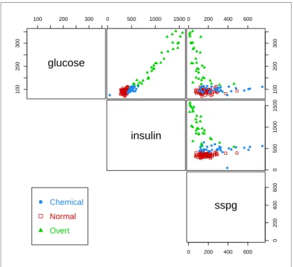
For example, consider thediabetesdataset which contains measurements on 145 non-obese adult subjects. Recorded variables areglucose, the area under plasma glucose curve after a three hour oral glucose tolerance test (OGTT),insulin, the area under plasma insulin curve after a three hour OGTT, andsspg, the steady state plasma glucose level. The patients are classified clinically into three groups.

> data(diabetes) > X <- diabetes[,2:4] > Class <- diabetes$class > table(Class)

Chemical Normal Overt

36 76 33

The data can be shown graphically (see Figure5) as follows:

> clp <- clPairs(X, Class, lower.panel = NULL)

> clPairsLegend(0.1, 0.3, class = clp$class, col = clp$col, pch = clp$pch)

The following function call can be used to compute the BIC for all the covariance structures and up to 9 components:

> BIC <- mclustBIC(X) > BIC

Bayesian Information Criterion (BIC):

EII VII EEI VEI EVI VVI EEE EVE

1 -5863.923 -5863.923 -5530.129 -5530.129 -5530.129 -5530.129 -5136.446 -5136.446 2 -5449.518 -5327.719 -5169.399 -5019.350 -5015.884 -4988.322 -5010.994 -4875.633

(8)

100 200 300 100 200 300

glucose

0 500 1000 1500 ● ● ●_● ● ●● ●● ● ●● ●● ●●● ●●●● ●●●●●● ● ● ●●● ● ● ● ● 0 200 400 600 100 200 300 ●_●●_● ● ● ● ● ● ● ● ● ● ● ●●● ● ● ● ●●● ●● ● ● ● ●● ●● ● ● ● ●

insulin

0 500 1000 1500 ●●●● ● ● ● ● ● ● ● ● ● ● ● _● ● ● ● ●_● ●●● ●_● ● ● ● ● ● ● ● ● ● ● 0 200 400 600 0 200 400 600

sspg

● _Chemical Normal Overt

Figure 5:Pairwise scatterplots for thediabetesdata with points marked according to classification.

3 -5412.588 -5206.399 -4998.446 -4899.759 -5000.661 -4827.818 -4976.853 -4858.851 4 -5236.008 -5208.512 -4937.627 -4835.856 -4865.767 -4813.002 -4865.864 -4793.261 5 -5181.608 -5202.555 -4915.486 -4841.773 -4838.587 -4833.589 -4882.812 NA 6 -5162.164 -5135.069 -4885.752 NA -4848.623 -4810.558 -4835.226 NA 7 -5128.736 -5129.460 -4857.097 NA -4849.023 NA -4805.518 NA 8 -5135.787 -5135.053 -4858.904 NA -4873.450 NA -4820.155 NA 9 -5150.374 -5112.616 -4878.786 NA -4865.166 NA -4840.039 NA

VEE VVE EEV VEV EVV VVV

1 -5136.446 -5136.446 -5136.446 -5136.446 -5136.446 -5136.446 2 -4920.301 -4877.086 -4918.500 -4834.727 -4823.779 -4825.027 3 -4851.667 -4775.537 -4917.567 -4809.225 -4817.884 -4760.091 4 -4840.034 -4794.892 -4887.406 -4823.882 -4828.796 -4802.420 5 NA NA -4908.030 -4842.077 NA NA 6 NA NA -4844.584 -4826.457 NA NA 7 NA NA -4910.155 -4852.182 NA NA 8 NA NA -4858.974 -4870.633 NA NA 9 NA NA -4930.535 -4887.206 NA NA

Top 3 models based on the BIC criterion:

VVV,3 VVE,3 EVE,4

-4760.091 -4775.537 -4793.261

In the results reported above, theNAvalues mean that a particular model cannot be estimated. This happens in practice due to singularity in the covariance matrix estimate and can be avoided using the Bayesian regularisation proposed inFraley and Raftery(2007a) and implemented inmclustas described inFraley et al.(2012). Optional arguments allow finetuning, such asGfor the number of components, andmodelNamesfor specifying the model covariances parameterisations (see Table3and

help(mclustModelNames)for a description of available model names). Another optional argumentx can be used to provide the output from a previous call tomclustBIC(). This is useful if the model space needs to be enlarged by fitting more models, e.g. by increasing the number of mixture components, without the need to recompute the BIC values for those models already fitted. Another usage of such strategy that may be helpful to users is provided inMclust(). For example, BIC values already available can be provided as follows

> Mclust(X, x = BIC)

Note that by specifying the argumentGandmodelNamesthe model space can be restricted to a subset, or enlarged to a superset. In the latter case the BIC is calculated only for the newly included models.

(9)

The use of BIC for model selection was available inmclustsince earlier versions. However, BIC tends to select the number of mixture components needed to reasonably approximate the density, rather than the number of clusters as such. For this reason, other criteria have been proposed for model selection, like theintegrated complete-data likelihood(ICL) criterion (Biernacki et al.,2000):

ICLM,G=BICM,G+2 n

∑

i=1 G

∑

k=1 ciklog(zik),

wherezikis the conditional probability thatxiarises from thekth mixture component, andcik=1 if the

ith unit is assigned to clusterkand 0 otherwise. ICL penalises the BIC through anentropyterm which measures clusters overlap. Provided that clusters overlapping is not too strong, ICL has shown good performance in selecting the number of clusters, with preference for solutions with well-separated groups.

Inmclustthe ICL can be computed by means of themclustICL()function:

> ICL <- mclustICL(X) > ICL

Integrated Complete-data Likelihood (ICL) criterion:

EII VII EEI VEI EVI VVI EEE EVE

1 -5863.923 -5863.923 -5530.129 -5530.129 -5530.129 -5530.129 -5136.446 -5136.446 2 -5450.004 -5333.689 -5169.732 -5023.533 -5016.010 -4994.986 -5012.758 -4876.295 3 -5415.983 -5219.627 -4999.693 -4910.963 -5011.423 -4839.130 -4985.448 -4875.992 4 -5238.797 -5224.698 -4939.741 -4847.524 -4876.784 -4823.308 -4867.650 -4809.169 5 -5190.524 -5226.204 -4923.986 -4865.230 -4854.347 -4859.162 -4895.412 NA 6 -5171.561 -5158.411 -4901.823 NA -4865.106 -4820.076 -4846.827 NA 7 -5136.220 -5152.330 -4872.644 NA -4870.151 NA -4817.584 NA 8 -5146.628 -5156.135 -4871.975 NA -4897.172 NA -4834.074 NA 9 -5180.744 -5145.708 -4911.346 NA -4883.199 NA -4872.677 NA

VEE VVE EEV VEV EVV VVV

1 -5136.446 -5136.446 -5136.446 -5136.446 -5136.446 -5136.446 2 -4927.621 -4885.421 -4920.413 -4844.590 -4826.796 -4834.539 3 -4866.976 -4793.271 -4927.563 -4821.068 -4828.535 -4776.086 4 -4869.658 -4823.020 -4956.077 -4847.034 -4839.703 -4830.658 5 NA NA -4948.787 -4869.279 NA NA 6 NA NA -4884.720 -4849.505 NA NA 7 NA NA -4947.190 -4878.445 NA NA 8 NA NA -4890.913 -4895.286 NA NA 9 NA NA -5007.250 -4919.228 NA NA

Top 3 models based on the ICL criterion:

VVV,3 VVE,3 EVE,4

-4776.086 -4793.271 -4809.169

As discussed above formclustBIC(), the output from a previous call tomclustICL()can be provided as input with the argumentxto avoid recomputing the ICL for models already fitted.

Both criteria can be shown graphically with (see Figure6):

> plot(BIC) > plot(ICL)

In this case BIC and ICL selected the same final model.

Other information criteria are available in the literature. For example, members of the Generalised Information Criteria (GIC) family (Konishi and Kitagawa,1996) are not computed by the package, but they can be easily obtained using the information returned by theMclust()function.

In addition to the information criteria just mentioned, the choice of the order of a mixture model for a specific component-covariances parameterisation can be carried out by likelihood ratio testing (LRT). Suppose we want to test the null hypothesisH0:G=G0against the alternativeH1:G=G1

for someG1 >G0; usually,G1 =G0+1 as it is a common procedure to keep adding components

sequentially. LetΨb_G_jbe the MLE ofΨcalculated underH_j:G=G_j(forj=0, 1). The likelihood ratio

test statistic (LRTS) can be written as

LRTS=−2 log{L(ΨbG0)/L(ΨbG1)}=2{`(ΨbG1)−`(ΨbG0)},

where large values of LRTS provide evidence against the null hypothesis. However, standard regularity conditions do not hold for the null distribution of the LRTS to have its usual chi-squared distribution

(10)

−5800 −5600 −5400 −5200 −5000 −4800 Number of components BIC ● ● ● ● ● ● ● ● ● ● ● ● ● ● ● ● ● ● ● ● ● ● ● ● ● ● ● ● ● 1 2 3 4 5 6 7 8 9 ● ● ● ● EII VII EEI VEI EVI VVI EEE EVE VEE VVE EEV VEV EVV VVV ₋₅₈₀₀ −5600 −5400 −5200 −5000 −4800 Number of components ICL ● ● ● ● ● ● ● ● ● ● ● ● ● ● ● ● ● ● ● ● ● ● ● ● ● ● ● ● ● 1 2 3 4 5 6 7 8 9 ● ● ● ● EII VII EEI VEI EVI VVI EEE EVE VEE VVE EEV VEV EVV VVV

Figure 6:Plots of BIC and ICL model selection criteria for thediabetesdata.

(McLachlan and Peel,2000, Chap. 6). As consequence, LRT significance is often estimated by a

resampling approach in order to produce ap-value. McLachlan(1987) proposed the using of the

bootstrap to obtain the null distribution of the LRTS. The bootstrap procedure is the following: 1. a bootstrap samplex∗_bis generated by simulating from the fitted model under the null hypothesis

withG0components, i.e. from the GMM distribution with the vector of unknown parameters

replaced by MLEs obtained from the original data underH0;

2. the test statistic LRTS∗_bis computed for the bootstrap samplex∗_bafter fitting GMMs withG0and

G1number of components;

3. steps 1. and 2. are replicated several times, sayB=999, to obtain the bootstrap null distribution of LRTS∗.

A bootstrap-based approximation to thep-value may then be computed as

p-value≈1+∑

B

i=1I(LRTS∗b≥LRTSobs)

B+1

where LRTSobsis the test statistic computed on the observed samplex, and I(·)denotes the indicator

function (which is equal to 1 if its argument is true and 0 otherwise).

The above bootstrap procedure is implemented in themclustBootstrapLRT()function. We need

to specify at least the input data and the model name we want to test:

> LRT <- mclustBootstrapLRT(X, modelName = "VVV") > LRT

Bootstrap sequential LRT for the number of mixture components ---Model = VVV Replications = 999 LRTS bootstrap p-value 1 vs 2 361.186445 0.001 2 vs 3 114.703559 0.001 3 vs 4 7.437806 0.938

The number of bootstrap resamples can be set by the optional argument nboot; if not provided,

nboot = 999is used. The sequential bootstrap procedure terminates when a test is not significant at the level specified bylevel(by default equal to0.05). There is also the option for a user to fix

the maximum number of mixture components to test via the argumentmaxG. In the example above

the bootstrapp-values clearly indicate the presence of three clusters. Note that models fitted on the original data are estimated via the EM algorithm initialised by the default model-based hierarchical agglomerative clustering. Then, during the bootstrap procedure, models under the null and the alternative hypotheses are fitted on bootstrap samples using again the EM algorithm. However, in this case the algorithm starts with the E step initialised with the estimated parameters obtained at the convergence of the EM algorithm on the original data.

(11)

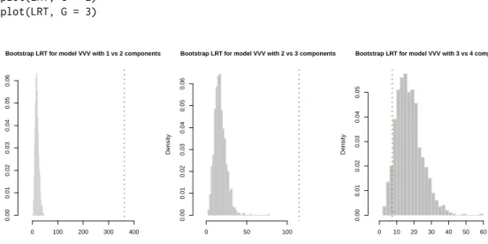
The bootstrap distributions of the LRTS can be shown graphically (see Figure7) using the associated plot method: > plot(LRT, G = 1) > plot(LRT, G = 2) > plot(LRT, G = 3) LRTS Density 0 100 200 300 400 0.00 0.01 0.02 0.03 0.04 0.05 0.06

Bootstrap LRT for model VVV with 1 vs 2 components

LRTS Density 0 50 100 0.00 0.01 0.02 0.03 0.04 0.05 0.06

LRTS Density 0 10 20 30 40 50 60 0.00 0.01 0.02 0.03 0.04 0.05

Figure 7:Histograms of LRTS bootstrap distributions for testing the number of mixture components in thediabetesdata. The dotted vertical lines refer to the sample values of LRTS.

Bootstrap inference

There are two main approaches to likelihood-based inference in mixture models, namely

information-based and resampling methods (McLachlan and Peel, 2000). In information-based methods, the

covariance matrix of the MLEΨbis approximated by the inverse of the observed information matrix

I−1₍

b Ψ), i.e.

Cov(Ψb)≈(I−1(Ψb)).

However, “the sample sizenhas to be very large before the asymptotic theory applies to mixture

models” (McLachlan and Peel,2000, p. 42). Indeed,Basford et al.(1997) found that standard errors obtained using the expected or the observed information matrix are unstable, unless the sample size is very large. For these reasons, they advocate the use of a resampling approach based on the bootstrap. For a recent review and comparison of different resampling approaches to inference in finite mixture models seeO’Hagan et al.(2015).

Thebootstrap(Efron,1979) is a general, widely applicable, powerful technique for obtaining an approximation to the sampling distribution of a statistic of interest. The bootstrap distribution is approximated by drawing a large number of samples (bootstrap samples) from the empirical distribution, i.e. by resampling with replacement from the observed data (nonparametric bootstrap), or from a para-metric distribution with unknown parameters substituted by the corresponding estimates (parametric bootstrap).

Let Ψb be the estimate of a set of GMM parametersΨ for a given modelM, i.e. covariance

parameterisation, and number of mixture componentsG. A bootstrap estimate of the corresponding

standard errors can be obtained using the following procedure:

• Obtain the bootstrap distribution for the parameters of interest by:

1. drawing a sample of sizenwith replacement from the empirical distribution(x1, . . . ,xn)

to form the bootstrap sample(x∗₁, . . . ,x∗_n);

2. fitting a GMM(M,G)to get the bootstrap estimatesΨb

∗

;

3. replicating steps 1–2 a large number of times, sayB, to obtainΨb

∗ 1,Ψb ∗ 2, . . . ,Ψb ∗ Bestimates fromBresamples.

• The bootstrap covariance matrix is then approximated by Covboot(Ψb)≈ 1 B−1 B

∑

b=1 (Ψb ∗ b−Ψb ∗ )(Ψb ∗ b−Ψb ∗ )>

(12)

whereΨb ∗ = 1 B B

∑

b=1 b Ψ∗b.

• The bootstrap standard errors for the parameter estimatesΨb are computed as the square root of

the diagonal elements of the bootstrap covariance matrix, i.e. seboot(Ψb) =

q

diag(Covboot(Ψb))

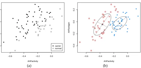
Consider thehemophiliadataset (Habbema et al.,1974) available in the packagerrcov, which contains two measured variables on 75 women belonging to two groups: 30 of them are non-carriers (normal group) and 45 are known hemophilia A carriers (obligatory carriers).

> data(hemophilia, package = "rrcov") > X <- hemophilia[,1:2]

> Class <- as.factor(hemophilia$gr)

> plot(X, pch = ifelse(Class == "normal", 1, 16))

> legend("bottomright", legend = levels(Class), pch = c(16,1), inset = 0.03)

The last command plots the observed data marked by the known classification (see Figure8a). In analogy with the analysis ofBasford et al.(1997, example II, Sec. 5), we fitted a two-components GMM with unconstrained covariance matrices:

> mod <- Mclust(X, G = 2, modelName = "VVV") > summary(mod, parameters = TRUE)

---Mclust VVV (ellipsoidal, varying volume, shape, and orientation) model with 2 components:

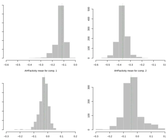
77.02852 75 11 106.5647 92.85533 Clustering table: 1 2 39 36 Mixing probabilities: 1 2 0.5108084 0.4891916 Means: [,1] [,2] AHFactivity -0.11627884 -0.36656353 AHFantigen -0.02457577 -0.04534792 Variances: [,,1] AHFactivity AHFantigen AHFactivity 0.01137602 0.00659927 AHFantigen 0.00659927 0.01239353 [,,2] AHFactivity AHFantigen AHFactivity 0.01585986 0.01505449 AHFantigen 0.01505449 0.03236079

Note that in thesummary()function call we used the optional argumentparameters = TRUEto retrieve the estimated parameters.

The clustering structure identified is shown in Figure8b and can be obtained as follows:

> plot(mod, what = "classification", main = FALSE)

Bootstrap inference for GMMs is available through the functionMclustBootstrap(), which

re-quires the user to input an object returned by a call toMclust(). Optionally, the user can also provide the number of bootstrap resamplesnbootand thetypeof bootstrap to perform. By default,nboot =

999andtype = "bs"for the nonparametric bootstrap. Thus, a simple call for computing the bootstrap distribution of the GMM parameters is the following:

(13)

● ● ● ● ● ● ● ● ● ● ● ● ● ● ● ● ● ● ● ● ● ● ● ● ● ● ● ● ● ● ● ● ● ● ● ● ● ● ● ● ● ● ● ● ● ● ● ● ● ● ● ● ● ● ● ● ● ● ● ● ● ● ● ● ● ● ● ● ● ● ● ● ● ● ● −0.6 −0.4 −0.2 0.0 −0.4 −0.2 0.0 0.2 AHFactivity AHF antigen ● ● carrier normal (a) −0.6 −0.4 −0.2 0.0 −0.4 −0.2 0.0 0.2 AHFactivity AHF antigen ● ● ● ● ● ● ● ● ● ● ● ● ● ● ● ● ● ● ● ● ● ● ● ● ● ● ● ● ● ● ● ● ●_●● ● ● ● ● (b)

Figure 8:True class membership (a) and estimated classification using GMM (b) for thehemophilia dataset.

> boot <- MclustBootstrap(mod, nboot = 999, type = "bs")

Note that for the sake of clarity we have included the argumentsnbootandtype, but they can be omitted since they are set at their defaults.

The functionMclustBootstrap()returns an object which can be plotted or summarised. For

instance, to graph the bootstrap distribution for the mixing proportions and for the component means we may use the code:

> par(mfrow = c(1,2)) > plot(boot, what = "pro") > par(mfrow = c(2,2)) > plot(boot, what = "mean") > par(mfrow = c(1,1))

The resulting plots are shown, respectively, in Figures9and10.

Mix. prop. for comp. 1

0.0 0.2 0.4 0.6 0.8 1.0

0

50

100

150

Mix. prop. for comp. 2

0.0 0.2 0.4 0.6 0.8 1.0

0

50

100

150

Figure 9:Bootstrap distribution for the mixture proportions. The vertical dotted lines refer to the

MLEs for the GMM fitted to thehemophiliadata.

A numerical summary of the bootstrap procedure is available through thesummarymethod, which by default returns the standard errors of GMM parameters:

> summary(boot, what = "se")

---Resampling standard errors

(14)

AHFactivity mean for comp. 1 −0.6 −0.5 −0.4 −0.3 −0.2 −0.1 0.0 0 100 200 300 400 500 600

AHFactivity mean for comp. 2

−0.6 −0.5 −0.4 −0.3 −0.2 −0.1 0.0 0 100 200 300 400 500

AHFantigen mean for comp. 1

−0.3 −0.2 −0.1 0.0 0.1 0.2 0 50 100 150 200 250

AHFantigen mean for comp. 2

−0.3 −0.2 −0.1 0.0 0.1 0.2

0

100

200

300

Figure 10:Bootstrap distribution for the mixture component means. The vertical dotted lines refer to the MLEs for the GMM fitted to thehemophiliadata.

Num. of mixture components = 2

Replications = 999

Type = nonparametric bootstrap

Mixing probabilities: 1 2 0.1249357 0.1249357 Means: 1 2 AHFactivity 0.04028375 0.04137370 AHFantigen 0.03262182 0.06456482 Variances: [,,1] AHFactivity AHFantigen AHFactivity 0.007018580 0.004690481 AHFantigen 0.004690481 0.003155312 [,,2] AHFactivity AHFantigen AHFactivity 0.005757398 0.005897374 AHFantigen 0.005897374 0.009654623

Thesummarymethod can also return bootstrap percentile confidence intervals. For the generic GMM parameterψofΨ, the percentile method yields the intervals[ψ_α∗_/2,ψ∗₁₋_α_/2], whereψ∗qis theqth

quantile (or the 100qth percentile) of the bootstrap distribution(ψb∗₁, . . . ,ψb∗_B). These can be obtained by

specifying in thesummarycall the argumentwhat = "ci"and, optionally, the confidence level of the intervals (by default,conf.level = 0.95). For instance:

> summary(boot, what = "ci")

(15)

---Resampling confidence intervals

---Model = VVV

Replications = 999

Type = nonparametric bootstrap

Confidence level = 0.95 Mixing probabilities: 1 2 2.5% 0.3193742 0.1785054 97.5% 0.8214946 0.6806258 Means: [,,1] AHFactivity AHFantigen 2.5% -0.22915526 -0.09784996 97.5% -0.07315876 0.02481681 [,,2] AHFactivity AHFantigen 2.5% -0.4573113 -0.1571624 97.5% -0.2747451 0.1318332 Variances: [,,1] AHFactivity AHFantigen 2.5% 0.004743597 0.007012672 97.5% 0.032144767 0.019245540 [,,2] AHFactivity AHFantigen 2.5% 0.003981163 0.006049076 97.5% 0.027297495 0.045854646

The functionMclustBootstrap()has also the provision for using the weighted likelihood boot-strap (Newton and Raftery,1994). This is a generalisation of the nonparametric bootstrap which assigns random (positive) weights to sample observations; it can be viewed as a generalized Bayesian bootstrap. The weights are obtained from a uniform Dirichlet distribution, i.e. by sampling from

nindependent standard exponential distributions and then rescaling by their average. Then, the

functionme.weighted()inmclustallows one to apply a weighted EM algorithm. This approach

may yield benefits when one or more components have small mixture proportions. In that case, a nonparametric bootstrap sample may have no representatives of them, but the weighted likelihood bootstrap will always have representatives of all groups.

In our data example the weighted likelihood bootstrap can be easily obtained by specifyingtype

= "wlbs"in theMclustBootstrap()function call:

> wlboot <- MclustBootstrap(mod, nboot = 999, type = "wlbs") > summary(wlboot, what = "se")

---Resampling standard errors

---Model = VVV

Replications = 999

Type = weighted likelihood bootstrap

Mixing probabilities: 1 2 0.1323612 0.1323612 Means: 1 2 AHFactivity 0.03977347 0.04192182 AHFantigen 0.02989056 0.06897928 Variances:

(16)

[,,1] AHFactivity AHFantigen AHFactivity 0.007074450 0.004686432 AHFantigen 0.004686432 0.003254011 [,,2] AHFactivity AHFantigen AHFactivity 0.005511614 0.005746981 AHFantigen 0.005746981 0.009883791

In this case the differences between the nonparametric and the weighted likelihood bootstrap are negligible. We can summarise the inference for the components means obtained under the two approaches with the following graphs of bootstrap percentile confidence intervals:

> boot.ci <- summary(boot, what = "ci") > wlboot.ci <- summary(wlboot, what = "ci") > par(mfrow = c(1,2), mar = c(4,4,1,1)) > for(j in 1:mod$G)

{ plot(1:mod$G, mod$parameters$mean[j,], col = 1:mod$G, pch = 15, ylab = colnames(X)[j], xlab = "Mixture component",

ylim = range(boot.ci$mean,wlboot.ci$mean), xlim = c(.5,mod$G+.5), xaxt = "n")

points(1:mod$G+0.2, mod$parameters$mean[j,], col = 1:mod$G, pch = 15) axis(side = 1, at = 1:mod$G)

with(boot.ci, errorBars(1:G, mean[1,j,], mean[2,j,], col = 1:G))

with(wlboot.ci, errorBars(1:G+0.2, mean[1,j,], mean[2,j,], col = 1:G, lty = 2)) } > par(mfrow = c(1,1)) −0.4 −0.3 −0.2 −0.1 0.0 0.1 Mixture component AHF activity 1 2 −0.4 −0.3 −0.2 −0.1 0.0 0.1 Mixture component AHF antigen 1 2

Figure 11:Bootstrap percentile intervals for the means of the GMM fitted to thehemophiliadataset. Solid lines refer to nonparametric bootstrap, dashed lines to the weighted likelihood bootstrap.

Initialisation of the EM algorithm

The EM algorithm is an easy to implement and numerically stable algorithm which has reliable global convergence under fairly general conditions. However, the likelihood surface in mixture models tends to have multiple modes and thus initialisation of EM is crucial because it usually produces sensible results when started from reasonable starting values (Wu,1983).

Inmclustthe EM algorithm is initialised using the partitions obtained from model-based hier-archical agglomerative clustering (MBHAC). In this approach, hierhier-archical clusters are obtained by recursively merging the two clusters that provide the smallest decrease in the classification likeli-hood for Gaussian mixture model (Banfield and Raftery,1993). Efficient numerical algorithms have

been discussed byFraley(1998). Using MBHAC is particularly convenient because the underlying

probabilistic model is shared by both the initialisation step and the model fitting step. Furthermore, MBHAC is also computationally advantageous because a single run provides the basis for initialising the EM algorithm for any number of mixture components and component-covariances

(17)

parameterisa-tions. Although there is no guarantee that the EM initialized by MBHAC will converge to the global optimum, it often provides reasonable starting points.

A problem with the MBHAC approach may arise in the presence of coarse data, resulting from the discrete nature of the data or from continuous data that are rounded when measured. In this case, ties must be broken by choosing the pair of entities that will be merged. This is often done at random, but regardless of which method is adopted for breaking ties, this choice can have important consequences because it changes the clustering of the remaining observations. Moreover, the final EM solution may depend on the ordering of the variables.

Consider the Flea beetles data available in packagetourr. This dataset provides six physical measurements for a sample of 72 flea beetles from three species:

> data(flea, package = "tourr") > X <- data.matrix(flea[,1:6])

> Class <- factor(flea$species, labels = c("Concinna","Heikertingeri","Heptapotamica")) > table(Class)

Class

Concinna Heikertingeri Heptapotamica

21 31 22

> col <- mclust.options("classPlotColors")[1:3]

> clp <- clPairs(X, Class, lower.panel = NULL, gap = 0,

symbols = c(16,15,17), colors = adjustcolor(col, alpha.f = 0.5)) > clPairsLegend(x = 0.1, y = 0.3, class = clp$class, col = col, pch = clp$pch,

title = "Flea beatle species")

As can be seen from Figure12, the observed values are rounded (to the nearest integer presumably) and there is a strong overplotting of points.

120 160 200 240 120 160 200 240 tars1 110 130 45 50 55 120 140 8 10 12 14 16 60 80 100 120 160 200 240 tars2 110 130 head 45 50 55 aede1 120 140 aede2 8 10 14 60 80 100 60 80 100 aede3 ●

Flea beatle species

Concinna

Heikertingeri Heptapotamica

Figure 12:Scatterplot matrix for the Flea beetles data with points marked according to the true classes.

> mod1 <- Mclust(X) > summary(mod1)

---Mclust EEE (ellipsoidal, equal volume, shape and orientation) model with 5 components:

(18)

Clustering table: 1 2 3 4 5 21 2 20 20 11 > adjustedRandIndex(Class, mod1$classification) [1] 0.7675713 > mod2 <- Mclust(X[,6:1]) > summary(mod2) ---Gaussian finite mixture model fitted by EM algorithm

-1287.027 74 55 -2810.777 -2812.702 Clustering table: 1 2 3 4 5 22 21 22 7 2 > adjustedRandIndex(Class, mod2$classification) [1] 0.8131206

By reversing the order of the variables in the fit ofmod2, the initial partitions differ due to ties in the data, so the EM algorithm converges to different solutions of the same EEE model with 5 components. The second solution has a higher BIC and better accuracy.

In situations like this we may want to assess the stability of results by randomly starting the

EM algorithm. The functionrandomPairs()may be called to obtain a random hierarchical structure

suitable to be used as initial clustering partition:

> mod3 <- Mclust(X, initialization = list(hcPairs = randomPairs(X, seed = 123))) > summary(mod3)

-1298.211 74 48 -2803.017 -2807.713 Clustering table: 1 2 3 4 16 15 22 21 > adjustedRandIndex(Class, mod3$classification) [1] 0.7867056

Using a random start we obtain a EEE model with 4 components, which has a higher BIC but a lower

ARI. However, a better initialisation may be found using the approach discussed inScrucca and

Raftery(2015). The main idea is to project the data through a suitable transformation which enhances separation among clusters before applying the MBHAC at the initialisation step. Once a reasonable hierarchical partition is obtained, the EM algorithm is run using the data on the original scale. For instance, a GMM started using the scaled SVD transformation is obtained with the following code:

> mod4 <- Mclust(X, initialization = list(hcPairs = hc(X, use = "SVD"))) > summary(mod4)

(19)

1 2 3 21 31 22

> adjustedRandIndex(Class, mod4$classification) [1] 1

In this case we achieve both the highest BIC and a perfect classification of the fleas into the actual species.

We conclude by noting that in the case of large datasets, i.e. having a large number of observations or cases, a subsample of the data can be used in the MBHAC phase before applying the EM algorithm to the full data set. This is easily done by providing an optional argument toMclust()ormclustBIC() (as well as many other functions) as a vector, says, of logical values or numerical indices specifying the subset of data to be used in the initial hierarchical clustering phase:

> Mclust(X, initialization = list(subset = s))

Density estimation

Density estimation plays an important role in applied statistical data analysis and theoretical research. Finite mixture models provide a flexible semi-parametric model-based approach to density estimation, which makes it possible to accurately approximate any given probability distribution.mclustprovides a simple interface to Gaussian mixture models for univariate and multivariate density estimation.

Izenman and Sommer(1988) considered the fitting of a Gaussian mixture to the distribution of the thickness of stamps in the 1872 Hidalgo stamp issue of Mexico2. A density estimate based on GMM can be obtained using the functiondensityMclust():

> data(Hidalgo1872, package = "MMST") > Thickness <- Hidalgo1872$thickness

> Year <- rep(c("1872", "1873-74"), c(289, 196)) > dens <- densityMclust(Thickness)

> summary(dens$BIC) Best BIC values:

V,3 V,5 V,4

BIC 2983.791 2974.939223 2972.19349 BIC diff 0.000 -8.852019 -11.59775 > summary(dens, parameters = TRUE)

---Density estimation via Gaussian finite mixture modeling

---Mclust V (univariate, unequal variance) model with 3 components:

1516.632 485 8 2983.791 2890.914 Clustering table: 1 2 3 128 171 186 Mixing probabilities: 1 2 3 0.2661410 0.3011217 0.4327374 Means: 1 2 3 0.07215458 0.07935341 0.09919740 Variances: 1 2 3 0.000004814927 0.000003097694 0.000188461484

2_{The Hidalgo stamp data is available at the home page for the book by}_Izenman₍₂₀₀₈_{) at}_{http://astro.temple.}

edu/~alan/MMST/datasets.html, or through the packageMMST. The latter has been archived on CRAN, so it must be installed using the following code:

> install.packages("http://cran.r-project.org/src/contrib/Archive/MMST/MMST_0.6-1.1.tar.gz", repos = NULL, type = "source")

(20)

The model selected is a three-component mixture with different variances. A graph of the density estimated is shown in Figure13a and is obtained with the code:

> br <- seq(min(Thickness), max(Thickness), length = 21) > plot(dens, what = "density", data = Thickness, breaks = br)

Here a histogram of the observed data is also drawn by providing the optional argumentdataand

with breakpoints between histogram cells specified in the argumentbreaks. From the graph, three modes appear at the means of the mixture components: one with larger stamp thickness, and two corresponding to thinner stamps.

Additional information can also be used. In particular, thickness measurements can be grouped according to the year of consignment; the first 289 stamps refer to the 1872 issue, and the remaining 196 stamps to the years 1873–1874. We may draw a (suitable scaled) histogram for each year-of-consignment and then add the estimated components densities as follows:

> h1 <- hist(Thickness[Year == "1872"], breaks = br, plot = FALSE) > h1$density <- h1$density*prop.table(table(Year))[1]

> h2 <- hist(Thickness[Year == "1873-74"], breaks = br, plot = FALSE) > h2$density <- h2$density*prop.table(table(Year))[2]

> x <- seq(min(Thickness)-diff(range(Thickness))/10,

max(Thickness)+diff(range(Thickness))/10, length = 200) > cdens <- predict(dens, x, what = "cdens")

> cdens <- t(apply(cdens, 1, function(d) d*dens$parameters$pro))

> col <- adjustcolor(mclust.options("classPlotColors")[1:2], alpha = 0.3)

> plot(h1, xlab = "Thickness", freq = FALSE, main = "", border = FALSE, col = col[1], xlim = range(x), ylim = range(h1$density, h2$density, cdens))

> plot(h2, add = TRUE, freq = FALSE, border = FALSE, col = col[2]) > matplot(x, cdens, type = "l", lwd = 1, add = TRUE, lty = 1:3, col = 1) > box()

The result is shown in Figure13b. Stamps from 1872 show a two-regime distribution, with one

corresponding to the component with the largest thickness, and one whose distribution essentially overlaps with the bimodal distribution of stamps for the years 1873–1874.

Thickness Density 0.06 0.08 0.10 0.12 0.14 0 20 40 60 (a) Thickness Density 0.06 0.08 0.10 0.12 0.14 0 10 20 30 40 50 60 70 (b)

Figure 13:(a) Histogram with mixture-based density estimate curve, and (b) histograms by group-year with estimated mixture-component densities, for theHidalgo1872stamps dataset.

As an example of bivariate density estimation, consider the well-known ‘Old Faithful’ data set

which provides the waiting time between eruptions (waiting) and the duration of the eruptions

(eruptions) for the Old Faithful geyser in Yellowstone National Park, Wyoming, USA. The dataset can be read and data plotted as follows:

> data(faithful)

> plot(faithful, cex = 0.5)

A bivariate density estimate for the Faithful data is obtained with the commands:

> dens <- densityMclust(faithful) > summary(dens)

(21)

● ● ● ● ● ● ● ● ● ● ● ● ● ● ● ● ● ● ● ● ● ● ● ● ● ● ● ● ● ● ● ● ● ● ● ● ● ● ● ● ● ● ● ● ● ● ● ● ● ● ● ● ● ● ● ● ● ● ● ● ● ● ● ● ● ● ● ● ● ● ● ● ● ● ● ● ● ● ● ● ● ● ● ● ● ● ● ● ● ● ● ● ● ● ● ● ● ● ● ● ● ● ● ● ● ● ● ● ● ● ● ● ● ● ● ● ● ● ● ● ● ● ● ● ● ● ● ● ● ● ● ● ● ● ● ● ● ● ● ● ● ● ● ● ● ● ● ● ● ● ● ● ● ● ● ● ● ● ● ● ● ● ● ● ● ● ● ● ● ● ● ● ● ● ● ● ● ● ● ● ● ● ● ● ● ● ● ● ● ● ● ● ● ● ● ● ● ● ● ● ● ● ● ● ● ● ● ● ● ● ● ● ● ● ● ● ● ● ● ● ● ● ● ● ● ● ● ● ● ● ● ● ● ● ● ● ● ● ● ● ● ● ● ● ● ● ● ● ● ● ● ● ● ● ● ● ● ● ● ● ● ● ● ● ● ● ● ● ● ● ● ● 1.5 2.0 2.5 3.0 3.5 4.0 4.5 5.0 50 60 70 80 90 eruptions w aiting (a) eruptions w aiting 1.5 2.0 2.5 3.0 3.5 4.0 4.5 5.0 50 60 70 80 90 ● ● ● ● ● ● ● ● ● ● ● ● ● ● ● ● ● ● ● ● ● ● ● ● ● ● ● ● ● ● ● ● ● ● ● ● ● ● ● ● ● ● ● ● ● ● ● ● ● ● ● ● ● ● ● ● ● ● ● ● ● ● ● ● ● ● ● ● ● ● ● ● ● ● ● ● ● ● ● ● ● ● ● ● ● ● ● ● ● ● ● ● ● ● ● ● ● ● ● ● ● ● ● ● ● ● ● ● ● ● ● ● ● ● ● ● ● ● ● ● ● ● ● ● ● ● ● ● ● ● ● ● ● ● ● ● ● ● ● ● ● ● ● ● ● ● ● ● ● ● ● ● ● ● ● ● ● ● ● ● ● ● ● ● ● ● ● ● ● ● ● ● ● ● ● ● ● ● ● ● ● ● ● ● ● ● ● ● ● ● ● ● ● ● ● ● ● ● ● ● ● ● ● ● ● ● ● ● ● ● ● ● ● ● ● ● ● ● ● ● ● ● ● ● ● ● ● ● ● ● ● ● ● ● ● ● ● ● ● ● ● ● ● ● ● ● ● ● ● ● ● ● ● ● ● ● ● ● ● ● ● ● ● ● ● ● ● ● ● ● ● ● (b) 2.0 2.5 3.0 3.5 4.0 4.5 5.0 50 60 70 80 90 eruptions w aiting (c) eruptions w aiting Density (d)

Figure 14:Plot of the Old Faithful data (a), mixture-based density estimate contours (b), image plot of density estimate (c) and perspective plot of the bivariate density estimate (d).

---Density estimation via Gaussian finite mixture modeling

1 2 3

130 97 45

Model selection based on the BIC selects a three-component mixture with common covariance matrix (EEE). One component is used to model the group of observations having both low duration and low waiting times, whereas two components are needed to approximate the skewed distribution of the observations with larger duration and waiting times.

Figure14b-d shows some of the available graphs inmclustfor a bivariate density estimated by GMM. These can be obtained with the commands:

> plot(dens, what = "density", data = faithful, grid = 200, points.cex = 0.5, drawlabels = FALSE)

> plot(dens, what = "density", type = "image", col = "steelblue", grid = 200) > plot(dens, what = "density", type = "persp", theta = -25, phi = 20,

border = adjustcolor(grey(0.1), alpha.f = 0.3))

Note that the same procedure using the functionmclustDensity()can also be used to obtain

(22)

Supervised classification

In supervised classification or discriminant analysis the aim is to build a classifier (or a decision rule) which is able to assign an observation with an unknown class membership to one ofKknown classes. For building a supervised classifier, a training dataset{(x1,y1), . . . ,(xn,yn)}is used for which both

the featuresxiand true classesyi∈ {C1, . . . ,CK}are known.

Mixture-based discriminant analysis models assume that the density for each class follows a Gaussian mixture distribution

fk(x) =

Gk

∑

g=1

πgkφ(x;µ_gk,Σgk),

whereπgkare the mixing probabilities for classk(πgk>0,∑gG=k1πgk=1),µ_gkthe means for component

gwithin classk, andΣgkthe covariance matrix of componentgwithin classk.Hastie and Tibshirani

(1996) proposed Mixture Discriminant Analysis (MDA) where it is assumed that the covariance matrix is the same for all the classes but is otherwise unconstrained, i.e.Σgk=Σfor allgandk. The number

of mixture components is assumed known for each class.

Bensmail and Celeux (1996) proposed the Eigenvalue Decomposition Discriminant Analysis

(EDDA) which assumes that the density for each class can be described by a single Gaussian component (i.e.Gk=1 for allk) with the component covariance structure factorised as

Σk=λkDkAkD>k.

Several models can be obtained from the above decomposition. IfΣk=λDAD>(model EEE), then

EDDA is equivalent to linear discriminant analysis (LDA). IfΣk = λkDkAkD>k (model VVV) then

EDDA is equivalent to quadratic discriminant analysis (QDA).

Consider the UCI Wisconsin breast cancer diagnostic data available athttp://archive.ics.uci.

edu/ml/datasets/Breast+Cancer+Wisconsin+(Diagnostic). This dataset provides data for 569

pa-tients on 30 features of the cell nuclei obtained from a digitized image of a fine needle aspirate (FNA) of a breast mass (Mangasarian et al.,1995). For each patient the cancer was diagnosed as malignant or benign. FollowingFraley and Raftery(2002) we considered only three attributes: extreme area, extreme smoothness, and mean texture. The dataset can be downloaded from the UCI repository using the following commands:

> data <- read.csv("http://archive.ics.uci.edu/ml/machine-learning-databases/breast-cancer-wisconsin/wdbc.data", header = FALSE)

> X <- data[,c(4, 26, 27)]

> colnames(X) <- c("texture.mean", "area.extreme", "smoothness.extreme") > Class <- data[,2]

Then, we may randomly assign approximately 2/3 of the observations to the training set, and the remaining ones to the test set:

> set.seed(123)

> train <- sample(1:nrow(X), size = round(nrow(X)*2/3), replace = FALSE) > X.train <- X[train,] > Class.train <- Class[train] > table(Class.train) Class.train B M 238 141 > X.test <- X[-train,] > Class.test <- Class[-train] > table(Class.test) Class.test B M 119 7 1

The functionMclustDA()provides fitting capabilities for the EDDA model, but we must specify the optional argumentmodelType = "EDDA". The function call is thus the following:

> mod1 <- MclustDA(X.train, Class.train, modelType = "EDDA") > summary(mod1, newdata = X.test, newclass = Class.test)

---Gaussian finite mixture model for classification

(23)

---EDDA model summary: log.likelihood n df BIC -2989.967 379 12 -6051.185 Classes n Model G B 238 VVI 1 M 141 VVI 1

Training classification summary: Predicted

Class B M

B 237 1

M 19 122

Training error = 0.05277045 Test classification summary:

Predicted

Class B M

B 116 3

M 5 66

Test error = 0.04210526

The EDDA mixture model selected by BIC is the VVI model, so each group is described by a single Gaussian component with varying volume and shape, but same orientation aligned with the coordinate axes. Note that in thesummary()function call we also provided the features and the known classes for the test set, so both the training error and the test error are reported. A cross-validation error can also be computed using thecvMclustDA()function, which by default usenfold = 10for a 10-fold cross-validation:

> cv <- cvMclustDA(mod1) > unlist(cv[c("error", "se")])

error se

0.052770449 0.007930516

EDDA imposes a single mixture component for each group. However, in certain circumstances

more complexity may improve performance. A more general approach, calledMclustDA, has been

proposed byFraley and Raftery(2002), where a finite mixture of Gaussian distributions is used within each class, with number of components and covariance matrix structures (expressed following the usual decomposition) being different between classes. This is the default model fitted byMclustDA:

> mod2 <- MclustDA(X.train, Class.train)

> summary(mod2, newdata = X.test, newclass = Class.test)

---Gaussian finite mixture model for classification ---MclustDA model summary:

log.likelihood n df BIC

-2937.586 379 29 -6047.361 Classes n Model G

B 238 EEV 2 M 141 VVI 2

Class B M

(24)

M 7 134

Predicted

Class B M

B 114 5

M 2 69

Test error = 0.03684211

A two-component mixture distribution is fitted to both the benign and malignant observations, but with different covariance structures within each class. Both the training error and the test error are slightly smaller than for EDDA, a fact also confirmed by the 10-fold cross-validation procedure:

> cv <- cvMclustDA(mod2) > unlist(cv[c("error", "se")])

error se

0.021108179 0.007648168

A plot method which produces a variety of graphs is associated with objects returned byMclustDA. For instance, pairwise scatterplots between the features, showing both the known classes and the estimated mixture components, are drawn as follows (see Figure15a–c):

> plot(mod2, what = "scatterplot", dimens = c(1,2)) > plot(mod2, what = "scatterplot", dimens = c(2,3)) > plot(mod2, what = "scatterplot", dimens = c(3,1))

Another interesting graph can be obtained by projecting the data on a dimension reduced subspace (Scrucca,2014) with the commands:

> drmod2 <- MclustDR(mod2) > summary(drmod2)

---Dimension reduction for model-based clustering and classification ---Mixture model type: MclustDA

Classes n Model G B 238 EEV 2 M 141 VVI 2 Estimated basis vectors:

Dir1 Dir2 Dir3

texture.mean -0.00935540 -0.044384467 -0.0006607120 area.extreme 0.00049997 0.000071676 -0.0000088494 smoothness.extreme 0.99995611 -0.999014521 0.9999997817

Dir1 Dir2 Dir3

Eigenvalues 0.67718 0.28159 0.013928 Cum. % 69.61869 98.56810 100.000000

> plot(drmod2, what = "boundaries", ngrid = 200)

The graph produced by the last command is shown in Figure15d. The two groups are largely separated along the first direction, with the group of malignant cases showing a higher variability.

Finally, note that the MDA model is equivalent to MclustDA withΣk=λDAD>(model EEE) and

fixedGk≥1 for eachk=1, . . . ,K. For instance, a MDA with two mixture components for each class

can be fitted as:

> mod3 <- MclustDA(X.train, Class.train, G = 2, modelNames = "EEE") > summary(mod3, newdata = X.test, newclass = Class.test)

---Gaussian finite mixture model for classification

(25)

---10 15 20 25 30 35 40 1000 2000 3000 4000 texture.mean area.e xtreme ● ● ● ● ● ● ● ● ● ● ● ● ● ● ●_● ●● ● ● ● ● ● ● ● ● ● ● ● ● ● ● ● ● ● ● ● ● ● ● ● ● ● ● ● ● ● ● ● ● ● ● ● ● ● ● ● ● ● _●●●● ● ● ● ● ●● ● ● ● ● ● ● ● ● ● ● ● ● _● _● ● ● ● ● ● ● ● ● ● ● ● ● ● ● ● ●● ● ● ● ● ● ● ● ● ● ● ● ● ● ● ● ● ● ● ● ● ● ● ● ● ● ● ● _● ● ● ● ● ● ● ● ● ● ● ● ● ● ● ● ● ● ● ● ● ● ● ● ● ● ● ● ● ● ● ● ● ● ● ●_● ● ● ● ● ● ● ● ● ●● ● ● ● ● ● ● ● ● ● ● ● ● ● ● ● ● ● ● ● ● ● ● ● ● ● ● ● ● ● ● ● ● ● ● ● ● ● ● ● ● ● ● ● ● ● ● ● ● ● ● ● ● ●● ● _● ● ● ● ● ● ● ● ● (a) 1000 2000 3000 4000 0.08 0.10 0.12 0.14 0.16 0.18 0.20 0.22 area.extreme smoothness .e xtreme ● ● ● ● ● ● ● ● ● ● ● ● ● ● ● ● ● ● ● ●_● ● ● ● ● ● ● ● ● ● ● ● ● ● ● ● ● ● ● ● ● ● ● ● ● ● ● ● ● ● ● ● ● ● ● ● ●_● ● ●● ● ● ● ● ● ● ● ● ● ● ● ● ● ● ● ● ● ● ● ● ●● ● ● ● ● ● ● ● ● ● ● ● ● ● ● ● ● ● ● ● ● ● ● ● ● ● ● ● ● ● ● ● ● ● ● ● ● ● ● ● ● ● ● ● ● ● ● ● ● ● ● ● ● ● ● ● ● ● ● ● ● ● ● ● ● ● ● ● ● ● ● ● ● ● ● ● ● ● ● ● ● ● ● ● ● ● ● ● ● ● ● ● ● ● ● ● ● ● ● ● ● ● ● ● ● ● ● ● ● ● ● ● ● ● ● ● ● ● ● ● ● ● ● ● ● ● ● ● ● ● ● ● ● ● ● ● ● ● ● ● ● ● ● ● ● ● ● ● ● ● ● ● ● ● ● ● (b) 0.08 0.10 0.12 0.14 0.16 0.18 0.20 0.22 10 15 20 25 30 35 40 smoothness.extreme te xture .mean ● ● ● ● ● ● ● ● ● ● ● ● ● ● ● ● ● ● ● ● ● ● ● ● ● ● ● ● ● ● ● ● ● ● ● ● ● ● ● ● ● ● ● ● ● ● ● ● ● ● ● ● ● ● ● ● ● ● ● ● ● ● ● ● ● ● ● ● ● ● ● ● ● ● ● ● ● ● ● ● ● ● ● ● ● ● ● ● ● ● ● ● ● ● ● ● ● ● ● ● ● ● ● ● ● ● ● ● ● ● ● ● ● ● ● ● ● ● ● ● ● ● ● ● ● ● ● ● ● ● ● ● ● ● ● ● ● ● ● ● ● ● ● ● ● ● ● ● ● ● ● ● ● ● ● ● ● ● ● ● ● ● ●● _● ● ● ● ● ● ● ● ● ● ● ● ● ● ● ● ● ● ● ● ● ● ● ●● ● ● ● ● ● ● ● ● ● ● ● ● ● ● ● ● ● ● ● ● ● ● ● ● ● ● ● ● ● ● ● ● ● ● ● ● _● ● ● ● ● ● ● ● ● ● ● ● ● (c) 0.0 0.5 1.0 1.5 −0.8 −0.6 −0.4 −0.2 0.0 0.2 0.4 Dir1 Dir2 ● ● ● ● ● ● ● ● ● ●●_● ● ● ● ● ● ● ● ● ● ● ● ● ● ● ● ● ● ● ● ● ● ● ● ● ● ● ● ● ● ● ● ● ● ● ● ● ● ● ● ● ● ● ● ● ● ● ● ● ● ● ● ● ● ● ● ● ● ● ● ● ● ● ● ● ● ● ● ● ● ● ● ● ● ● ● ● ● ● ● ● ● ● ● ● ● ● ● ● ● ● ● ● ● ● ● ● ● ● ● ●● ● ● ● ● ● ● ● ● ● ● ● ● ● ● ● ● ● ● ● ● ● ● ● ● ● ● ● ● ● ● ● ● ● ● ● ● ● ● ● ● ● ● ● ● ● ● ● ● ● ● ● ● ● ● ● ●● ● ● ●● ● ● ● ● ● ● ● ● ● ● ● ● ● ● ● ● ● ● ● ● ● ● ● ● ● ● ● ● ● ●● ● ● ● ● ● ● ● ● ● ● ● ● ● ● ● ● ● ● ● ●● ●●● ● ● ● ● ● ● ● ● ● (d)

Figure 15:Pairwise scatterplots between variables for the Wisconsin breast cancer data (panels a–c). Points are marked by cancer diagnosis (benign =•, malignant =), whereas ellipses correspond to covariances of mixture components estimated withMclustDA. Plot of data projected along the first two estimated directions obtained withMclustDR, and uncertainty classification boundaries (d).

MclustDA model summary:

log.likelihood n df BIC

-2968.077 379 26 -6090.531 Classes n Model G

B 238 EEE 2 M 141 EEE 2

Class B M

B 235 3

M 12 129

Predicted

Class B M