Volume 11 | Issue 1
Article 14
5-1-2012
Parameter Estimation with Mixture Item Response
Theory Models: A Monte Carlo Comparison of
Maximum Likelihood and Bayesian Methods
W. Holmes Finch
Ball State University, [email protected]
Brian F. French
Washington State University, [email protected]
Follow this and additional works at:
http://digitalcommons.wayne.edu/jmasm
Part of the
Applied Statistics Commons
,
Social and Behavioral Sciences Commons
, and the
Statistical Theory Commons
This Regular Article is brought to you for free and open access by the Open Access Journals at DigitalCommons@WayneState. It has been accepted for inclusion in Journal of Modern Applied Statistical Methods by an authorized administrator of DigitalCommons@WayneState.
Recommended Citation
Finch, W. Holmes and French, Brian F. (2012) "Parameter Estimation with Mixture Item Response Theory Models: A Monte Carlo Comparison of Maximum Likelihood and Bayesian Methods,"Journal of Modern Applied Statistical Methods: Vol. 11: Iss. 1, Article 14. Available at:http://digitalcommons.wayne.edu/jmasm/vol11/iss1/14
167
Parameter Estimation with Mixture Item Response Theory Models:
A Monte Carlo Comparison of Maximum Likelihood and Bayesian Methods
W. Holmes Finch
Brian F. French
Ball State University, Muncie, IN
Washington State University, Pullman, WA
The Mixture Item Response Theory (MixIRT) can be used to identify latent classes of examinees in data as well as to estimate item parameters such as difficulty and discrimination for each of the groups. Parameter estimation via maximum likelihood (MLE) and Bayesian estimation based on the Markov Chain Monte Carlo (MCMC) are compared for classification accuracy and parameter estimation bias for difficulty and discrimination. Standard error magnitude and coverage rates were compared across number of items, number of latent groups, group size ratio, total sample size and underlying item response model. Results show that MCMC provides more accurate group membership recovery across conditions and more accurate parameter estimates for smaller samples and fewer items. MLE produces narrower confidence intervals than MCMC and more accurate parameter estimates for larger samples and more items. Implications of these results for research and practice are discussed.
Key words: Mixture item response theory, differential item functioning, Bayesian estimation, Markov chain Monte Carlo estimation, maximum likelihood estimation.
Introduction
Mixture item response theory (MixIRT) has become an increasingly popular tool for investigating a variety of issues in educational and psychological assessment (Cohen & Bolt, 2005; Bolt, Cohen & Wollack, 2001). Use of the MixIRT model in a variety of contexts has been described in detail by a number of authors (Cohen & Bolt, 2005; von Davier & Yamamoto, 2004; von Davier & Rost, 1995; Mislevy & Verhelst, 1990; Rost, 1990; Yamamoto, 1987). For example, MixIRT has been recommended for identifying subsets of a population (latent
W. Holmes Finch is Professor of Psychology in the Department of Educational Psychology, and Educational Psychology Director of Research in the Office of Charter School. Email him at: [email protected]. Brian F. French is Associate Professor and Co-Director Learning and Performance Research Center Washington State University. Email him at: [email protected].
classes) which are characterized by different item response models for a particular measure or instrument (Li, et al., 2009). In this context, psychometricians have used MixIRT to detect and characterize differential item functioning (DIF) (Cohen & Bolt, 2005; De Ayala, et al., 2002; Bolt, Cohen & Wollack, 2002, 2001). This simulation study compares the parameter estimation accuracy for two methods of estimation used with MixIRT: Maximum Likelihood Estimation (MLE) and Baysian estimation using the Markov Chain Monte Carlo (MCMC) approach.
Prior research has demonstrated the utility of the MixIRT framework given its ability to identify differentially responding subgroups that exist organically in the data. This approach stands in contrast to the assumption that differential response patterns are inherently linked to easily identified grouping variables (e.g., gender) and that all (or most) members of such intact groups will demonstrate very similar responses to items; an assumption which underlies other statistical models used for similar purposes. For example, in the detection of DIF using standard methods such as logistic
168
regression or the Mantel-Haenszel test, comparisons of item response patterns are made between known groups such as males and females. However, recent work in the area of DIF has demonstrated that the causes of DIF are often complex and not so clearly tied to easily identified groups (Cohen & Bolt, 2005). In such cases, the utility of the MixIRT approach – and its sometimes superiority – has been demonstrated in gaining a deeper understanding into differential item response patterns such as those associated with DIF (Maij-de Meij, Kelderman & van der Flier, 2010; Samuelson, 2008; Cohen, Cho & Kim, 2005; Rost, 1990).
The MixIRT model, which combines the powerful statistical tools of latent class analysis (LCA) and item response theory (IRT), assumes that a population is composed of a finite number of latent examinee classes that can be differentiated based upon their item response patterns (Rost, 1997). In turn, these different response patterns will manifest themselves as differences in parameters of the item response model associated with each group. The 2-parameter MixIRT (Mix2PL) model for dichotomous data takes the following form:
(
1 ,
)
(
(
( ( ))
))
1
jg ig jg jg ig jg a b ig a be
P U
g
e
θ θθ
− −= |
=
+
(1)Here latent class membership (g = 1, 2, …, G), within class difficulty for item j (bjg) within class discrimination for item j (ajg), and the within class level on the latent trait being measured for person i (θig) are all model parameters to be estimated. In addition, each survey respondent is placed in a latent class, and the proportions of individuals in each class (πg), are also estimated, under the constraint that
1
1
G g gπ
==
. Variants of this model including a pseudo-chance parameter (Mix3PL) and excluding both pseudo-chance and constraining discrimination to be equivalent across items (Mix1PL) are also available, as in the standard IRT context. The focus of this study is on dichotomous items for which chance responding is not applicable, such as behavior inventories; for this reason only the Mix1PL and Mix2PL models are examined.The item parameter values carry the same meaning in the MixIRT context as in the more general IRT framework; thus, item difficulty provides information regarding the likelihood that an individual will endorse an item (or answer it correctly in the context of cognitive assessment), discrimination indicates how well the item differentiates between individuals with different levels of the construct being measured and pseudo-guessing is a measure of the likelihood that an examinee would respond to the item correctly due solely to chance (de Ayala, 2009).
When there are class differences in the item difficulty and discrimination parameter values, researchers conclude that members of the latent classes perform differently on the specific item (Cohen & Bolt, 2005). For example, assume that the results of the analysis indicate the presence of two distinct latent classes in the population. In this case, if a specific item for latent class 1 has a higher value for bjg than class 2, it is known that the item is more difficult for class 1; this in turn may provide insights into the types of individuals who tend to be in that class. Similarly, if latent class 2 has a higher ajg value on an item compared to class 1, it can be concluded that the item is better able to differentiate among individuals with different levels of the latent trait for class 2 than for class 1. This approach to using MixIRT models has been particularly evident in the identification and characterization of DIF for achievement tests (Cohen & Bolt, 2005), though it has also been used to identify different usage patterns of the not sure category in personality inventories (Maij-de Meij, Kelderman & van der Flier, 2008) and to identify individuals engaging in impression management in organizational surveys (Eid & Zickar, 2007).
Parameter Estimation
In the literature, model parameter estimation for MixIRT models has been examined using both MLE (Willse, 2011) and MCMC methods in the Bayesian context (von Davier & Rost, 2007). Excellent discussions regarding the technical details of both approaches are present in the literature; the interested reader is referred to von Davier and Carstensen (2007) for a thorough treatment of a number of MixIRT models available. Although
169
prior applied work has used both methods, there has been very little research empirically comparing the performance of the two estimation techniques to one another.
Based upon these prior applications, each approach has been shown to have specific advantages and disadvantages in practice. For example, MCMC has proven useful with complex MixIRT models because it does not require integration of the likelihood function (as does MLE) which can be extremely difficult when it is necessary to estimate many parameters (Junker, 1999).
Conversely, the MCMC approach is often very time consuming to implement (sometimes taking 10 days or more to fit a single model), and may encounter difficulties in converging to solutions for individual parameters (Li, et al., 2009). The issue of time is non-trivial when dealing with MixIRT models, as several different latent class solutions must typically be fit and then compared in order to determine which is optimal for the data at hand (Li, et al., 2009). MLE does not usually require such large amounts of time as MCMC and MLE has been used successfully in estimating MixIRT models (von Davier & Rost, 2007); however, MLE can mistakenly converge on localized, rather than general maximum likelihood solutions, leading to suboptimal model parameter estimates. This problem can be overcome through the use of multiple random starting values, such as the 10 random starts used in this study (Rost, 1991). Of concern, though, is that using more starting values and increasing the maximum number of iterations in order to increase the probability of obtaining optimal fit, also increases the time necessary for the model to converge and provide parameter estimates.
Although relatively little work has been done explicitly comparing the performance of MLE and MCMC estimation techniques in the context of MixIRT models, Li, et al. (2009) conducted a simulation study in which they examined the performance of MCMC primarily in terms of identifying the optimal model selection criterion for dichotomous item response data. However, as a part of this study, MixIRT parameter estimation was also examined. Results of their research indicated
that item parameter recovery was worse in the presence of more latent classes and better when there were more items and/or more examinees. Recovery of latent class membership was generally greater than 80%, with the most accurate results for the Mix2PL model and the least accurate for the Mix3PL.
Cho and Cohen (2010) expanded on this work by investigating item parameter recovery for the multilevel Mix1PL model, in which information at both the student (level 1) and school (level 2) levels were taken into consideration. The estimation used in this simulation study was also MCMC and the model was restricted to the 1-Parameter Logistic form. The authors reported that recovery of both the item difficulty estimates and group membership was good for the MCMC methodology used in the study. A study by Willse (2011) examined the performance of a joint maximum likelihood estimator for the Rasch MixIRT model. He reported the results of a simulation study that showed good parameter recovery for group specific item difficulty values. No other simulation work examining the accuracy of parameter estimates in the MixIRT context was identified in the literature.
The goal of this simulation study is to compare the parameter recovery performance of the MLE and MCMC estimation procedures in the context of the MixIRT model for dichotomous item response data. Prior simulation work in this area has focused primarily on MCMC estimation and has not directly compared the ability of this approach and MLE in terms of parameter recovery accuracy, both for the items and for latent class membership. In addition, this work adds the additional simulation conditions of group size ratio, which has not been previously examined. Thus, this study adds to the literature by directly comparing these two popular methods of estimation across a range of conditions for dichotomous item response data. Prior applied work in this area has shown both methods to be potentially useful in many cases. However, given that both have distinct certain practical advantages in terms of their relative abilities to converge on the optimal solution and the time needed to use each; it would be helpful to understand whether one technique provides any
170
methodological advantages over the other and, if so, under what conditions. If one approach does provide greater parameter estimation accuracy, researchers might be able to make decisions regarding which to use in light of this and the aforementioned practical concerns. Given that such a direct comparison has not been previously published, it is believed that this work will add valuable information to the literature on MixIRT models.
Methodology
The simulation study used to compare the parameter estimation accuracy for MLE and MCMC, involved the manipulation of several factors that have been shown pertinent in previous research. A total of 50 replications per combination of manipulated conditions were generated. The two estimation methods were fit using Mplus version 6.1 (Muthén & Muthén, 2011). Several of the simulation conditions used in this study were based on those reported in Li, et al. (2009). These were selected for use because they were used previously and have been shown to be related to the performance of the MCMC estimator.
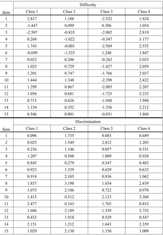
Thus, given that something is known about how the MCMC approach performs under the various conditions, it was determined that they would be particularly informative for the comparison of this method and MLE. It should be noted that the simulating item parameter values were drawn from item responses to a behavioral checklist given to adolescents through the auspices of the 2009 administration of the Youth Risk Behavior Survey (Centers for Disease Control, 2009). A MixIRT study involving these items was published by Finch and Pierson (2011) in which they report results for four latent classes based on 16,000 adolescents’ responses (yes or no) to items asking about participation in a variety of risky sexual and substance use behaviors. These data were fit with a Mix2PL model. The population item parameter values used in the generation of simulated data for the current study were drawn from this earlier work and are shown in Table 1. Manipulated Conditions
A total of 2, 3, and 4 latent classes were simulated with sample sizes of 400, 1,000 and
2,000 examinees. Group sizes were either equal or unequal. In the unequal case for two groups, the ratio was 75/25, for three groups the ratio was 50/25/25 and for four groups the ratio was 40/20/20/20. Two models were simulated, the Mix1PL and Mix2PL, and the appropriate model was fit for each replication. Specifically, when the Mix2PL model was used to generate the data, the Mix2PL model was fit to each simulated dataset. Finally, three conditions were simulated for the number of items, 5, 15 and 30. These were intended to simulate very short, moderate and somewhat longer instruments. The underlying latent trait was simulated to be unidimensional from the N(0,1) distribution.
In order to differentiate the groups in the simulations, the item discrimination and item difficulty parameter values for the groups were made to differ (Table 1 shows the values for each group). For the 5 item condition, the first 5 item parameter sets were used, and for the 30 item condition, the 15 item set was used twice, in keeping with the methodology laid out in Li, et al. (2009). The outcome variables of interest were the proportion of correctly placed individuals into the latent classes, the estimation bias for item difficulty and discrimination, mean standard error for parameters across replications and the coverage rates for the item parameters. In order to place all items on the same metric prior to estimating the outcome variables, methods outlined by Lloyd and Hoover (1980) were utilized.
Model Convergence Issues
Researchers using the MCMC approach to estimation must ensure that each time an analysis is run the results converge to the optimal solution. As a part of this, a burn-in period must be established, which means identifying a number of draws from the posterior distribution that will be ignored as the estimator seeks to converge to the solution for each parameter. After the burn-in has been established, samples are then drawn from subsequent values in the posterior in order to obtain the final parameter estimate. Based upon earlier work in this area, particularly that of Li, et al. (2009) and Cho and Cohen (2010), as well as examination of auto-correlation plots from several of the simulated datasets, 10,000
171
Table 1: Item Difficulty and Discrimination Parameters Used In the Monte Carlo Simulations
Item
Difficulty
Class 1 Class 2 Class 3 Class 4
1 2.817 1.188 -2.522 1.824 2 -1.447 0.099 0.306 1.054 3 -2.507 -0.835 -2.002 2.819 4 0.268 -1.022 -0.547 3.177 5 1.743 -0.001 -2.569 2.535 6 -0.699 -1.525 1.248 1.847 7 0.022 0.206 -0.262 2.025 8 1.025 0.729 -1.627 2.059 9 1.201 0.747 -1.766 2.037 10 1.444 1.348 -2.398 2.422 11 1.299 0.867 -2.085 2.207 12 1.056 0.681 -1.725 2.233 13 0.713 0.626 -1.048 1.948 14 1.154 0.352 -1.536 2.212 15 0.546 0.001 -0.851 1.868 Item Discrimination
Class 1 Class 2 Class 3 Class 4
1 0.096 1.735 0.083 0.689 2 0.025 1.549 2.812 1.203 3 0.236 1.146 0.057 0.351 4 1.207 0.568 1.009 0.928 5 0.845 0.279 0.547 0.483 6 0.923 1.339 0.629 0.632 7 0.918 2.105 0.836 1.062 8 1.857 3.198 1.654 2.459 9 1.075 2.106 0.722 0.978 10 1.415 0.512 2.133 3.304 11 2.477 0.163 1.765 0.853 12 1.606 2.189 1.359 2.752 13 0.432 1.918 0.529 0.547 14 2.151 1.212 1.643 2.359 15 1.029 2.130 1.150 1.009
172
iterations were used as the burn-in, 10,000 post burn-in values were used to obtain parameter estimates with MCMC and thinning of the posterior draws was set at 50.
Each method presented some difficulties in terms of convergence. The MLE approach had difficulty converging for the smallest sample size condition (400). Therefore additional simulations were run until the necessary 50 converged replicates were obtained for MLE. With respect to MCMC, difficulty was encountered in obtaining convergence for the 5 item condition for some of the replications. Thus, as with the MLE method, additional replications were run until the requisite 50 converged solutions were obtained. Although it was recognized that both conditions causing these problems (400 examinees and 5 items) might generally be viewed as problematic in practice, it is important to learn as much as possible about the relative performance of these two methods, including under relatively difficult circumstances such as these, given that such conditions are not uncommon in actual research practice, particularly for behavioral inventories and short mental health screening instruments. Label Switching
An issue of some importance in any study involving latent class analysis is that of label switching, in which a given latent class might take one number (e.g., 1) in one case, and another number (e.g., 2) in another case. In reality, however, the group is constituted of the same individuals or type of individuals. In a simulation study involving MCMC estimation, label switching consists of two separate problems. First, within the context of Bayesian analysis, label switching can occur across repeated sampling from the posterior distribution within a single analysis. In order to detect this type of label switching, it is necessary to monitor the posterior densities of group membership. A multimodal distribution would be indicative of such label switching. During the simulation the densities were monitored and multimodal solutions did not present themselves, thus this type of label switching was eliminated as a concern.
The second type of label switching occurs across replications of a simulation study
and is not limited to MCMC but can also occur for MLE. Essentially, it involves changing the arbitrary group label as described, but in this case from one replication to another. For this study, the methodology described in Cho, Cohen and Kim (2006) was used. Namely, the item parameter estimates from the individual sample replications were compared with those used to generate the data and the group labels from the sample replications were changed to match those to which they most closely conformed from the model generation groups.
Results Classification Accuracy
In order to identify statistically significant effects among the manipulated factors described, a repeated measures analysis of variance (ANOVA) was used. The within replication variable was method, and the between replication variables were the manipulated factors including number of items, sample size, number of groups, group size ratio and the underlying model. The dependent variable was the mean classification accuracy across replications. In addition to statistical significance, effect sizes were also calculated for all main effects and interactions.
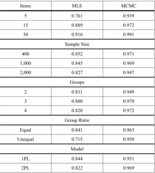
ANOVA results for the classification accuracy outcome variable indicate that the method of estimation interacted significantly with number of items (F < 0.001, η2= 0.363), number of subjects (F = −0.025, η2= 0.07), group size ratio (F = 0.006, η2= 0.117) and number of groups (F = 0.003, η2= 0.108). In addition, method (F < 0.001, η2= 0.721) itself was statistically significant. Table 2 shows the classification accuracy rates for each of the manipulated variables by method. Across all other conditions, the MCMC approach yielded more accurate group classification than did MLE. This difference was most noticeable for fewer items, with the gap between the two estimation techniques narrowing as the number of items increased, in large part due to improvements in the accuracy of MLE. In addition, the MLE approach was more accurate at classifying individuals when the groups were of equal size, whereas the MCMC was largely impervious to the group size ratio. Across
173
conditions MCMC yielded similar rates of correct classification, which were uniformly higher than 0.9, whereas MLE was much more likely to be influenced by the manipulated conditions and rarely had correct classification rates greater than 0.9.
Item Discrimination Parameter Estimation
As with the classification accuracy results, ANOVA was used to identify significant study effects with regard to bias in the estimation of the item discrimination parameter.
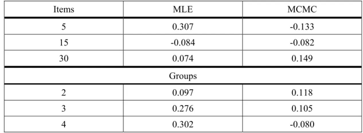
The interaction terms of method by number of items (F = 0.025, η2= 0.07) and method by number of groups (F < 0.001, η2= 0.147) were significantly related to bias in the a
parameter estimate. Table 3 shows the mean bias results across replications for these two terms. Regardless of the number of items, the Bayesian method provided estimates of a with bias under 0.15 in all cases. By contrast, MLE yielded very biased estimates in the case of 5 items, had comparable bias to the Bayesian for 15 items,
Table 2: Latent Class Classification Accuracy by Method, Number of Items, Number of Groups, Sample Size, Group Size Ratio and Underlying Model
Items MLE MCMC 5 0.761 0.939 15 0.889 0.972 30 0.916 0.991 Sample Size 400 0.852 0.971 1,000 0.845 0.969 2,000 0.827 0.947 Groups 2 0.831 0.949 3 0.880 0.970 4 0.820 0.972 Group Ratio Equal 0.841 0.963 Unequal 0.715 0.950 Model 1PL 0.844 0.951 2PL 0.822 0.969
174
and had lower bias for 30 items. With respect to the number of groups, item discrimination bias for MLE increased concomitantly with increasing number of groups. In contrast, estimation accuracy for the Bayesian approach seemed largely unaffected by the number of groups in terms of the absolute size of bias, though for 4 groups the estimates were somewhat underestimated whereas for 2 and 3 groups they were somewhat overestimated.
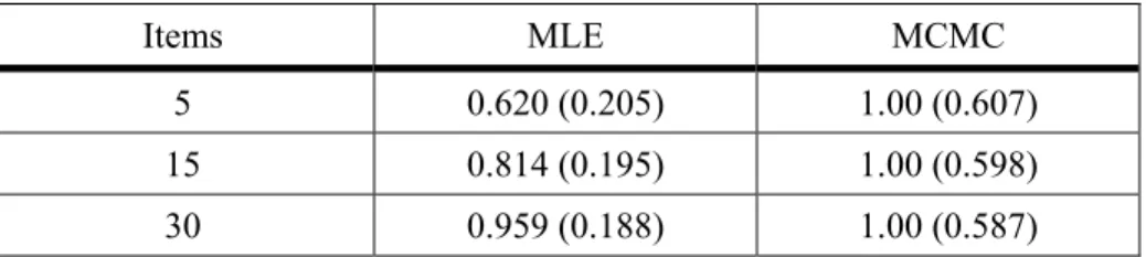
In addition to parameter estimation bias, the coverage rates for the discrimination parameters were also estimated. These coverage rates represent the proportion of simulation replications for which the nominal 95% confidence interval actually contained the true population value of a: ideally they would be 0.95. The results of the ANOVA indicated that the main effect of method (F < 0.001, η2=
0.762), as well as the interaction of method by number of items (F < 0.001, η2= 0.339) were statistically significant. Table 4 includes the coverage rates for each method by the number of items.
Across conditions, the coverage rates for the MCMC estimates were near 1.0 and were much higher than those of the MLE method. The latter estimation approach had higher coverage for tests with a larger number of items, though in no case were these rates comparable to those of the MCMC approach and they were generally lower than the nominal 0.95 level. The standard errors of these estimates also appear in Table 4, and show that those associated with MCMC were larger than those from MLE. These larger standard errors resulted in wider confidence intervals for the MCMC estimates, which contributed in part to the higher coverage rates for this approach.
Table 3: Item Discrimination Bias by Method, Number of Items and Number of Groups
Items MLE MCMC 5 0.307 -0.133 15 -0.084 -0.082 30 0.074 0.149 Groups 2 0.097 0.118 3 0.276 0.105 4 0.302 -0.080
Table 4: Item Discrimination Coverage Rates (Mean Standard Error across Replications) By Method and Number of Items
Items MLE MCMC
5 0.663 (0.394) 0.991 (0.902)
15 0.788 (0.378) 1.000 (0.886)
175
Item Difficulty Parameter Estimation
The ANOVA results for the item difficulty parameter bias revealed that only the interaction of method by number of groups was statistically significant (F = 0.013, η2= 0.082). Table 5 includes the b bias results for this interaction term. For both methods, underestimation bias of the b parameter increased concomitantly with increases in the number of groups. The significant interaction appears to be a function of the fact that for 2 groups, the bias in the MCMC estimator was somewhat smaller than that of MLE; however, for 3 groups this pattern was reversed and for 4 groups the bias of the two methods was comparable.
The ANOVA for the b parameter coverage rates showed that the main effect of method (F < 0.001, η2= 0.768) and the interaction of method by number of items (F < 0.001, η2= 0.263) were the two significant terms in this model. Table 6 includes the coverage rates for b by method and number of items. Item difficulty coverage rates were uniformly 1.0 for the MCMC estimator, whereas for MLE these rates were below the nominal 0.95 level except for the 30 item condition. An
examination of the average standard error for these estimates, also shown in Table 6, reveals that the MCMC estimator had a substantially larger standard error than did MLE, which in turn led to wider confidence intervals. Therefore, although the coverage rates for the MCMC approach were higher than those of MLE, the associated intervals were also wider, just as was the case for item discrimination.
Conclusion
It is hoped that the results of this study will prove useful to researchers and practitioners interested in using the MixIRT approach in order to gain a greater understanding of their data, whether in the context of characterizing DIF, or identifying specific item response profile groups, as was the case for the study upon which this work was built, or gaining further insights into the interplay of personality and item response profiles. In all of these cases, accurate estimation of item response and group membership parameters is crucial to obtaining useful results that can inform policy and practice. Prior applied research has focused on two different estimation methods, MCMC within the Bayesian framework, and MLE, and
Table 5: Item Difficulty Bias by Method and Number of Groups
Groups MLE MCMC
2 -0.029 -0.019
3 -0.031 -0.038
4 -0.057 -0.055
Table 6: Item Difficulty Parameter Coverage Rates (Mean Standard Error across Replications) by Method and Number of Items
Items MLE MCMC
5 0.620 (0.205) 1.00 (0.607)
15 0.814 (0.195) 1.00 (0.598)
176
has shown that both approaches appear to be useful for specific situations. In addition, a very brief simulation literature demonstrated some support for the MCMC technique in terms of parameter estimation, though no direct comparisons with MLE were made. At the same time, these earlier authors noted that the MCMC approach often requires a very lengthy time period in order to complete a single analysis (Li, et al., 2009), a fact which has also been reported by other authors. Therefore, while previous work indicates that the MCMC estimation approach might hold promise in terms of parameter estimation, the logistics of using it in many real world situations might limit its practical value. Given that there has been little simulation work examining MixIRT in general, and no studies that could be found comparing the two major parameter estimation approaches with one another, this the current study should prove informative to practitioners considering the use of the MixIRT paradigm in research.
Study results herein indicate that for correctly identifying which group an individual belongs to, the MCMC approach would seem to be more effective. Across virtually all conditions simulated, it was more accurate than MLE in terms of correct group identification. Across all simulated conditions, MCMC correctly classified respondents in over 96% of cases, whereas MLE was correct only 84% of the time. Furthermore, there was very little variation in the rates of accuracy for MCMC across manipulated conditions, however, for MLE the accuracy rates varied greatly, particularly as a function of the number of items. Thus, for researchers whose primary goal is to gain insights into the types of respondents present in the population, it would seem that MCMC is the preferable estimation approach.
For researchers who are most interested in the accuracy and precision of class specific item difficulty and discrimination values, the results of the study are somewhat more ambiguous. It seems that with respect to item discrimination estimates, the MCMC approach might provide somewhat less biased estimates for shorter instruments. By contrast, item discrimination bias was lower for MLE when the instrument contained 30 items. With respect to item difficulty, the length of the instrument was
not as salient as the number of latent classes, such that the presence of more groups was associated with greater item difficulty bias for both methods. It is possible that this relationship was due in part to the smaller number of individuals in the groups that was present when the number of groups increased.
In terms of estimate precision as measured by the average standard error value across replications and the coverage rates, MLE appears to have fared somewhat better than MCMC. It is true that the coverage rates for MCMC were uniformly higher than those of MLE, but this appears to have been due in the main to the larger standard errors associated with the Bayesian estimates. Thus, researchers using MCMC can be reasonably sure that the credible intervals for the estimates contain the population parameter value, but they also must be aware that these intervals will generally be wide. Such wide intervals may not be terribly informative to researchers interested in obtaining fairly precise estimates of the item difficulty and discrimination values.
Recommendations for Practice
Based on study results, some general recommendations for practice can be developed. First, when there are many items, the MLE approach might be optimal. With 30 items, MLE produced somewhat more accurate item parameter estimates than did MCMC and it had group classification accuracy rates above 90% (though this was lower than that of MCMC). In addition to the more accurate item parameter estimation in the presence of 30 items, MLE estimates were also more precise than those of MCMC, as witnessed in the narrower confidence intervals. However, when an instrument consists of very few items, MLE should probably be avoided, as it produced substantially more biased estimates than MCMC and will be less accurate in terms of classifying respondents. When researchers suspect that more than 3 groups are present, MCMC would also seem to be a better choice, particularly with regard to estimating item discrimination parameters. Such is not the case for item difficulty, which was compromised with equal severity for both estimation approaches for 4 groups. In short, situations in which many items are available to
177
describe many examinees and few groups are ideal for the use of MLE, whereas cases in which the number of items is small and/or the number of groups is large may be better suited to MCMC. All of these recommendations must be considered in light of the fact that the MCMC estimation will probably take substantially more time than will MLE.
Finally, with respect to using MixIRT models with relatively small samples as previously discussed, with a sample size of 400 individuals, both estimation methods had difficulty reaching convergence for many of the replications in the study. This was particularly an issue for MLE, though the Bayesian approach was also less successful for an N of 400 than for the larger sample sizes; thus, in practice researchers might find that they are unable to obtain useful estimates for this small sample size regardless of the method used. This problem was particularly acute for a larger number of groups in conjunction with the smaller sample size, because the number of individuals in each group became small. Therefore, one other recommendation for practice to come out of this study is that – for samples of 400 or fewer – MixIRT may not be particularly viable, except perhaps for the simplest models.
Limitations and Areas for Future Research As with any research, this study has some limitations which impact interpretations of the results that must be acknowledged. First, the Mix3PL model was not included in the study. This decision was made consciously, as the focus of the study was on instruments that are common in psychology, such as behavior inventories and personality assessments, for which chance responding is a negligible issue. In addition, the item parameter values used to generate the data were based on a behavior inventory. That this focus is believed to be appropriate for research in psychology, but it does limit the findings for those interested in cognitive assessments where chance responses to items are an issue. Future research should include a Mix3PL model. In addition, the current study examined a limited range of unequal group size conditions. Although this is the first study in this area to manipulate group sizes, it is recognized that more work in this area needs to
be conducted and thus a wider range of unequal group size conditions should be simulated. In addition, it is believed that the settings of the MCMC and MLE techniques used in this study were in keeping with recommended practice, it would be helpful if a wider array of values for the burn-in period and post burn-in iterations for MCMC were used and if more conditions in terms of number of random starts and convergence criteria were investigated for MLE. Such research would provide more information regarding the optimal settings for use with these estimators.
References
Bolt, D. M., Cohen, A. S., & Wollack, J. A. (2001). A mixture item response model for multiple-choice data. Journal of Educational and Behavioral Statistics, 26, 381-409.
Bolt, D. M., Cohen, A. S., & Wollack, J. A. (2002). Item parameter estimation under conditions of test speededness: Application of a mixture Rasch model with ordinal constraints.
Journal of Educational Measurement, 39, 331-348.
Centers for Disease Control. (2009).
Youth risk behavior survey: 2009 National YRBS data Users Manual. Atlanta, GA: Center for Disease Control.
Cho, S-J., & Cohen, A. S. (2010). A multilevel mixture IRT model with an application to DIF. Journal of Educational and Behavioral Statistics, 35(3), 336-370.
Cho, S-J., Cohen, A. S., & Kim, S-H. (2006). An investigation of priors on the probabilities of mixtures in the mixture Rasch model. Paper presented to the annual meeting of the Psychometric Society, Montreal, Canada.
Cohen, A. S., & Bolt, D. M. (2005). A mixture model analysis of differential item functioning. Journal of Educational Measurement, 42(2), 133-148.
Cohen, A. S., Cho, S.J., & Kim, S.H. (2005). A mixture testlet model for educational tests. Paper presented at the annual meeting of the American Educational Research Association, Montreal, Canada.
de, Ayala, R. J. (2009). The theory and practice of item response theory. New York, NY: The Guilford Press.
178
de Ayala, R. J., Kim, S. H., Stapleton, L. M., & Dayton, C. M. (2002). Differential item functioning: A mixture distribution conceptualization. International Journal of Testing, 2, 243-276.
Eid, M., & Zickar, M. (2007). Detecting response styles and faking in personality and organizational assessment by mixed Rasch models. In Multivariate and Mixture Distribution Rasch Models, M. vonDavier & C. Cartensen (Eds.), 255-270. New York: Springer.
Finch, W. H., & Pierson, E. E. (2011). A mixture IRT analysis of risky youth behavior.
Frontiers in Quantitative Psychology, 2,1-10. Junker, B. W. (1999). Some statistical models and computational methods that may be useful for cognitively-relevant assessment. Retrieved November 8, 2010, from http://citeseerx.ist.psu.edu/viewdoc/download?d oi=10.1.1.142.7053&rep=rep1&type=pd.
Li, F., Cohen, A. S., Seok-Ho, K., & Cho, S-J. (2009). Model selection methods for mixture dichotomous IRT models. Applied Psychological Measurement, 33(5), 353-373.
Maij-de Meij, A. M., Kelderman, H., & van der Flier, H. (2010). Improvement in detection of differential item functioning using a mixture item response theory model.
Multivariate Behavioral Research, 45(6), 975-999.
Mislevy, R. J., & Verhelst, N. D. (1990). Modeling item responses when different subjects employ different solution strategies.
Psychometrika, 55(2), 195-215.
Muthén, L. K. & Muthén, B. O. (2011).
MPlus software, version 6.1. Los Angeles, CA: MPlus.
Rost, J. (1997). Logistic mixture models. In Handbook of modern item response theory, W. J. van der Linden & R. K. Hambleton (Eds.), 449-463. New York, NY: Springer.
Rost, J. (1991). A logistic mixture distribution model for polychotomous item responses. British Journal of Mathematical and Statistical Psychology, 44, 75-92.
Rost, J. (1990). Rasch models in latent classes: An integration of two approaches to item analysis. Applied Psychological Measurement, 14, 271-282.
Samuleson, K. M. (2008). Examining differential item functioning from a latent class perspective. In Advances in latent variable mixture models, G. R. Hancock & K. M. Samuelson (Eds.), 67-113. Charlotte, NC: Information Age Publishing.
von Davier, M. & Rost, J. (1995). Polytomous mixed Rasch models. In Rasch models: Foundations, recent developments and applications, G. H. Fischer & I. W. Molenaar (Eds.), 371-379. New York, NY: Sprinter.
von Davier, M. & Carstensen, C.H. (2007). Multivariate and mixture distribution Rasch models. New York, NY: Springer.
von Davier, M., & Rost, J. (2007). Mixture distribution item response models. In
Handbook of statistics, 26: Psychometrics, C. R. Rao & S. Sinharay (Eds.), 643-661. Amsterdam: Elsevier.
von Davier, M., & Yamamoto, K. (2004). Partially observed mixture models of IRT models: An extension of the generalized partial credit model. Applied Psychological Measurement, 28, 389-406.
Willse, J. T. (2011). Mixture Rasch models with Joint Maximum Likelihood Estimation. Educational and Psychological Measurement, 17(1), 5-19.
Yamamoto, K. (1987). A model that combines IRT and latent class models. Unpublished doctoral dissertation, University of Illinois at Urbana-Champaign.