Energy Efficiency is not Enough,
Energy Proportionality is Needed!
Theo H¨arder, Volker Hudlet, Yi Ou, and Daniel Schall
Databases and Information Systems Group University of Kaiserslautern, Germany {haerder,hudlet,ou,schall}@cs.uni-kl.de
Abstract. Due to theenergy consumption/resource utilization
charac-teristics of todays centralized DB servers, the fastest configuration is also the most energy-efficient one. Extensive use of SSDs alone cannot enable a fundamental change of this overall picture, because the storage-related energy consumption is typically only a little fraction of the overall energy budget. Even, when this storage-related share is (almost) com-pletely reduced by optimized flash-aware buffer management, the saving effect achieved may be limited by less than∼10%. Therefore, we have designed a cluster of wimpy computing nodes called WattDB, where the individual nodes are dynamically attached and detached to the cluster on demand – depending on the current workload needs –, thereby aiming at energy-proportional DB management.
1
Introduction
In recent years, data management on new hardware evolved into an active and attractive field of research. Among the topics considered for data management are multi-core processors, vectorized query processing, flash memory, (column-oriented) main-memory databases, OLAP- or OLTP-specific optimizations, etc. Most efforts exclusively aim at performance enhancements for specific database applications – highlighted by the statement “One Size Does Not Fit All!”. Representative approaches include MonetDB [1], Greenplum [2], VoltDB [3], SanssouciDB [4], and others.
A few years ago, we started to explore the use of flash memory and the integration of SSDs (solid state disks) into the DB I/O architecture. Unlike most other projects, we primarily addressed energy efficiency for all tasks of database management, but also considered potential performance gains. Our strong hope was to improve both goals – “Keeping Performance While Saving Energy?” [5], which was supported by our initial experiments.
The remainder of this paper is organized as follows: Sect. 2 reviews indicative research results concerning our experiments of exploiting SSDs for DB manage-ment, whereas our findings concerning flash-aware DB buffers are summarized in Sect. 3. Sect. 4 highlights the need of energy proportionality. How such a goal can be approximated in DB applications, is sketched in Sect. 5, where we discuss design issues for ourWattDB system. Concluding remarks and future challenges are outlined in Sect. 6.
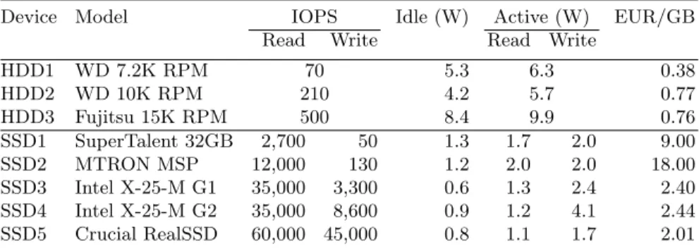
Table 1:Storage device characteristics
Device Model IOPS Idle (W) Active (W) EUR/GB Read Write Read Write
HDD1 WD 7.2K RPM 70 5.3 6.3 0.38 HDD2 WD 10K RPM 210 4.2 5.7 0.77 HDD3 Fujitsu 15K RPM 500 8.4 9.9 0.76 SSD1 SuperTalent 32GB 2,700 50 1.3 1.7 2.0 9.00 SSD2 MTRON MSP 12,000 130 1.2 2.0 2.0 18.00 SSD3 Intel X-25-M G1 35,000 3,300 0.6 1.3 2.4 2.40 SSD4 Intel X-25-M G2 35,000 8,600 0.9 1.2 4.1 2.44 SSD5 Crucial RealSSD 60,000 45,000 0.8 1.1 1.7 2.01
2
Experimental Results and Critical Observations
SSD ∕= SSD – this fact was drastically demonstrated in [6]. It is not only true when using a collection of different device types, but also for instances of the same device type. Reasons are continuous improvements of the SSD types as well as refinements of the flash translation layer (FTL) to optimize measures for wear leveling. All these optimization efforts are proprietary and kept as “business secrets” of the device manufacturers – resulting in a black-box view of SSD devices, often exhibiting surprising behavior. Table 1 gives an overview of the impressive success these efforts gained for almost all characteristics chosen.
Strong variations at the instance level are caused by the read/write/erase asymmetry which is amplified by the prevailing conditions or housekeeping tasks of an individual device, e. g., device “aging”, state-dependent garbage collection, frequency of erasures as reactions to load patterns, etc.
All these reasons lead to the conclusion that current, state-of-the-art SSDs cannot be easily integrated and used for database management. In any case, we have to cope in DB environments with a spectrum of heterogeneous SSDs with differing and instable access behavior. Furthermore, the data sheets of the device manufacturers often report performance figures which can never be met by typical DB workloads. To support our conclusion, we want to repeat here some indicative, empirical results of previous publications [6,7].
2.1 SSD Performance Measurements
Our initial experiments focused on DB-specific read and write performance of SSDs, for which the essential characteristics – taken from the data sheets of the manufacturers – are listed in Table 1. To stress all devices with the same access patterns, we developed a tool (similar to uFlip and IOmeter1) that allows us to
perform benchmarks on the devices. The tool supports adjustable page sizes and is able to read and write different access patterns from/to the devices; we used 32KB page sizes in all experiments2.
1
http://uflip.inria.fr/∼uFLIP/, http://www.iometer.org
2
‐ 1,000 2,000 3,000 4,000 5,000 6,000 RS RR RSS WS WR WSS SSD1 IOPS ‐ 1,000 2,000 3,000 4,000 5,000 6,000 RS RR RSS WS WR WSS SSD2 IOPS ‐ 1,000 2,000 3,000 4,000 5,000 6,000 RS RR RSS WS WR WSS SSD3 IOPS ‐ 1,000 2,000 3,000 4,000 5,000 6,000 RS RR RSS WS WR WSS SSD4 IOPS ‐ 1,000 2,000 3,000 4,000 5,000 6,000 RS RR RSS WS WR WSS SSD5 IOPS RS Read Sequential RR Read Random RSS Read Skip‐Sequential WS Write Sequential WR Write Random WSS Write Skip‐Sequential Legend
Fig. 1: Performance measurements using different SSD types
Our first test pattern is sequentially accessing𝑛 pages simulating DB scan operations. A second pattern is randomly accessing all pages of the test file, where each page is fetched only once. Finally, theskip-sequentialpattern accesses pages sequentially, but skips randomly over some pages. Hence, we mimic kind of index scans via (sorted) reference lists. Illustrated in Fig. 1, the results for the SSDs considered are briefly commented in the following:
– SSD1: Our results clearly show slow performance under all tested patterns as well as heavily degraded write performance. But, random read is as fast as sequential read.
– SSD2 shows improved performance to SSD1. Still, random writing is tremen-dously slower than other access methods.
– SSD3, as the first Intel generation, is really good at sequential reading, while random reading is comparatively slow. All write patterns are performing equally well – a significant operational difference w. r. t.SSD1 and SSD2.
– SSD4, as next Intel generation, came with the additional featureTRIM sup-port3. It reveals improved overall performance for all patterns. Nevertheless,
the disk is showing the same challenges as the first generation.
– While reading on SSD5 is faster than on all other SSDs we tested, random writing stresses this device remarkably. Although the data sheet promises 60,000 IOPS for random read, we could not get even close to this number (a fact we experienced in most other tests).
2.2 Result Interpretation
Using these performance results, we examine common assumptions, expert wis-dom, and rules of thumb regarding SSDs [9] and show that not all of them are true. Given that we cannot design a DBMS tailor-made to a single SSD of a specific type and that varying workloads are present, we may critically observe the following issues.
3
0 500 1000 1500 2000 2500 1 6 11 16 21 26 31 36 41 46 51 SSD3 random write IOPS sec Fig. 2: IOmeter per sec
0 500 1000 1500 2000 2500 3000 3500 1 6 11 16 21 26 31 36 41 46 51 SSD4 write after TRIM IOPS
sec Fig. 3: TRIM effects
Random access SSDs should not suffer from random access, in fact, they do. Random access may be substantially slower than sequential access.
Therefore, sequential accesses should still be preferred over random accesses, although it is not as vital as on hard disks. For hard disks, a rule of thumb recommends an index-based scan only if the selectivity factor of the predicate to be evaluated is below∼1–3%, otherwise a sequential scan of the whole table is advised. On SSDs, the selectivity factor can be shifted to higher percentages. Because of the different SSDs’ performance characteristics, it is not possible to spot a clear break-even point.
Database query optimizers can decide between random and sequential access based on configurable disk parameters.4 Simple rules of thumb, however, do
not work anymore [10], especially if the performance characteristics fluctuate over time. Therefore, optimizing algorithms under wrong assumptions or device models can make overall performance even worse. Furthermore, developers for flash-aware buffer algorithms have to consider that device-specific tweaks might be obsolete in no time.
Unstable and fluctuating behavior Using a tweaked IOmeter version, we
were able to get more detailed performance data from our devices. Fig. 2 visu-alizes the write performance of SSD3 in pages/second on a per-second basis. As illustrated, every 4 to 5 seconds, performance is heavily degraded for about 3 seconds. We conclude, the drive is performing internal reorganization like freeing up flash blocks or searching for another writable block.
While benchmarking SSD4, we had a look at the TRIM command intro-duced for this model and observed an interesting behavior. Fig. 3 depicts our write performance measurement right after deleting ∼130 GB of files on the drive and issuing corresponding TRIM commands to the drive. In this graph, a heavily degraded performance in the first half of the measurement is evident. Apparently, the SSD tries to free up flash blocks while we were simultaneously applying a write load to it. The proprietary FTL mapping particularly con-cerns device caching, block allocation, and garbage collection. All these mecha-nisms are software controlled and entirely hidden to the upper software layers.
4
E.g.: http://publib.boulder.ibm.com/infocenter/db2luw/v9r7/index.jsp? topic=/com.ibm.db2.luw.admin.perf.doc/doc/c0005051.html
Hence, optimization decisions in the OS or DBMS may be counterproductive and sometimes even worsen the time-consuming house-keeping activities. As in-ferred from Fig. 2, write latency may extremely vary. While less than ∼400 𝜇s in the best case, we have observed outliers of more than some hundred ms, that is a device-dependent variance of more than∼200–500. In contrast, disks with a device-dependent variance of∼2–5 exhibit quite stable access behavior and lend themselves to reliable optimizer decisions.
Another aspect is a kind of heterogeneity among the SSD types present in a DBMS environment, where several heterogeneous SSDs may coexist in an appli-cation (or they may be dynamically exchanged). As a consequence, tailor-made algorithms for specific SSD types, e. g., concerning indexing or buffer manage-ment, are not very useful. The same arguments apply for specific workload op-timizations (pure OLTP or OLAP processing, mixed workloads with varying degrees of reads/writes). A continuous adjustment or exchange of algorithms affected is not very practical in productive DBMS applications.
Read/write asymmetry It does not seem to be true in general. SSD1 and
SSD2, for example, do not exhibit degraded performance for (sequential) write, they are equally fast as sequential read. On all other SSDs, an asymmetry is measurable, but still not as bad as advertised. Exploited for buffer management, this observation may make at least some prevalent assumptions obsolete.
Slower when full? As a consequence of the erasures, overwriting some blocks on a full disk should be much slower than writing to an empty disk. We verified this assumption by filling all drives with random data and repeating our tests afterwards. No significant differences were measurable.
Impact of queue depth To gain more insights, we repeatedly measured various queue depths. By using a random read pattern, we give the FTLs a fair chance to optimize the queue. As reported in [6], the only significant improvement was observed between QD 1 and QD 2. Beyond this point, extending the QD did not improve data throughput. We did not expect this result, because manufacturers use even higher queue depths for their performance measurements.
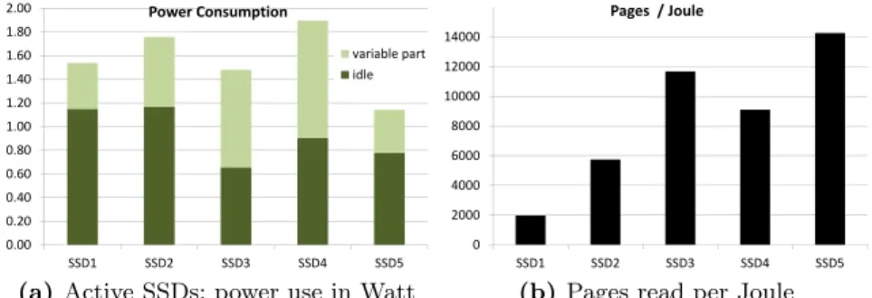
Energy consumption Fig. 4a shows the absolute power consumption of the
SSDs we tested. For this test, a sequential read pattern is used. Write patterns might consume even more energy. Obviously, the drives do consume energy when being idle; therefore, they are not as energy saving as expected. Power consump-tion ranges from ∼4–6 Watt for consumer disks to ∼9–14 Watt for disks of enterprise server quality. The SSDs’ power profiles are substantially different to those of hard disks; their power consumption for idle states and peak loads is con-siderably lower, for example, up to a factor of∼15 and∼8 for SSD3 and HDD3, respectively (see Table 1). Fig. 4b shows how many pages can be read by each SSD consuming one Joule of energy. As illustrated,𝑝𝑎𝑔𝑒𝑠/𝐽 𝑜𝑢𝑙𝑒 are constantly rising, thus newer SSDs are getting more energy efficient. On conventional disks
0.00 0.20 0.40 0.60 0.80 1.00 1.20 1.40 1.60 1.80 2.00 SSD1 SSD2 SSD3 SSD4 SSD5 Power Consumption variable part idle
(a) Active SSDs: power use in Watt
0 2000 4000 6000 8000 10000 12000 14000 SSD1 SSD2 SSD3 SSD4 SSD5 Pages / Joule
(b)Pages read per Joule
Fig. 4: Energy-related SSD measurements
we measured only∼600–1,800𝑝𝑎𝑔𝑒𝑠/𝐽 𝑜𝑢𝑙𝑒. Anyway, a more differentiated com-parison is cumbersome, because of the different performance characteristics and their implications on energy efficiency.
The critical question is whether these considerable differences of energy con-sumption at the device level cause perceptible energy saving at the system level. For this reason, we compare disk- and SSD-based DBMS buffer management in the next section.
3
Findings in DBMS Buffer Management
Because of the read/write/erase asymmetry, buffer management tailor-made to the SSD characteristics is a key issue for flash-aware DBMS optimizations. The fact “whether a page is read only or modified” is an even more performance-critical criterion for the replacement decision [11] than in disk-based DBMSs.
3.1 Objectives of Flash-Aware Replacement Algorithms
Even with SSDs, maintaining a high hit ratio – the primary goal of disk-based buffer algorithms – is still important, because the bandwidth of main memory is at least an order of magnitude higher than the interface bandwidth of storage devices. To exploit the SSD characteristics to the extent possible, flash-aware buffer management should observe the following basic principles [7]:
P1 Minimize the number of physical writes.
P2 Address write patterns to improve the write efficiency.
P3 Keep a relatively high hit ratio.
We have designed the CFDC (Clean-First Dirty-Clustered) algorithm [12] which perfectly addresses all these key issues. As our competitors, quite a number of flash-aware replacement algorithms were proposed trying to approximate these
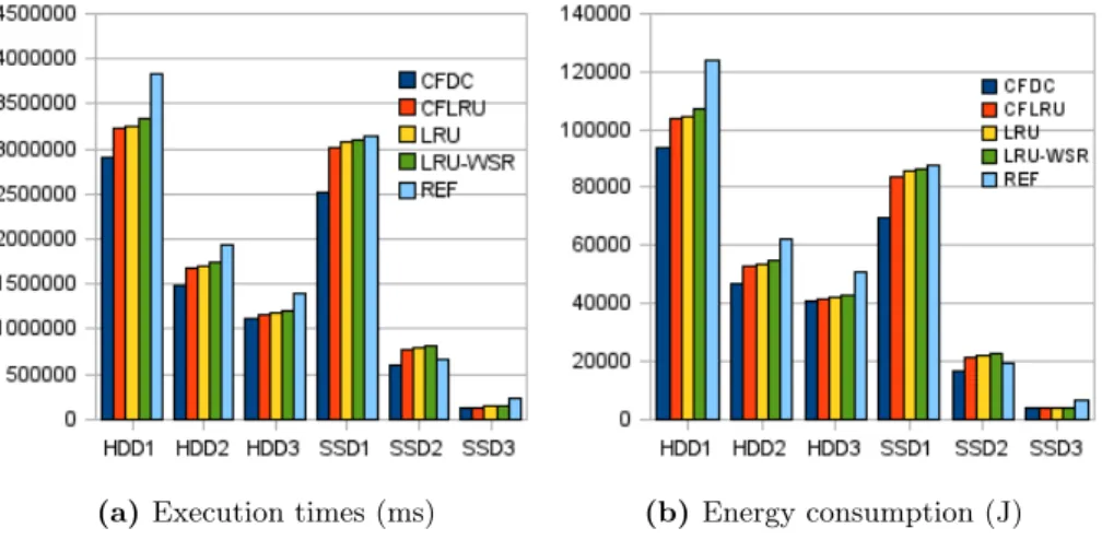
(a) Execution times (ms) (b)Energy consumption (J)
Fig. 5: Performance and energy consumption running the TPC-C trace
principles more or less successfully. Here, we cross-compare CFDC to the general-purpose algorithm LRU [11] and the algorithms CFLRU [13], LRU-WSR [14], and REF [15], which are tailor-made for SSD use.
Because DBMSs often use heterogeneous storage devices of mixed types, an important question needs to be answered: how well do these algorithms per-form on conventional magnetic disks? Furthermore, how much energy is used for buffer management in either case, i. e., how energy efficient are these algorithms in differing environments? Here, we want to repeat these answers given in [7], thereby preparing our arguments for energy-proportional DBMS management.
3.2 Experiments
Our test environment consists of an Intel Core2 Duo processor and 2 GB of main memory. Both the OS (Ubuntu Linux with kernel version 2.6.31) and the DB engine are installed on an IDE magnetic disk (system disk). The test data (as a DB file) resides on a separate magnetic disk/SSD (data disk, denoted as SATA). The data disks, as listed in Table 1, are chosen to represent low-end (HDD1/SSD1), middle-class (HDD2/SSD2), and high-low-end (HDD3/SSD3) devices. They are connected to the system one at a time.
Using a relational DBMS, we recorded an OLTP trace (a buffer reference string) of a 20-minutes TPC-C workload with a scaling factor of 50 warehouses. We ran the trace for each of the five algorithms under identical conditions and repeated it for each of the devices under test. Using a buffer size of 8000 pages (64 MB), we minimized the influence of the device caches. But, not the absolute but the relative differences are most expressive.
The illustration of the recorded execution times and energy consumptions in Fig. 5 is considered to be indicative for what we can expect as typical behavior and optimization potential under the various storage device settings. The differ-ence between the execution times of the algorithms becomes smaller on SSD3
(a) HDD3 (b) SSD3
Fig. 6: Break-down of average power (W)
(see Fig. 5) due to two reasons: 1. The I/O cost on SSD3 is much smaller than on other devices, yielding the buffer layer optimization less significant; 2. This device has supposedly the largest device cache, since it is the newest product among the devices tested.
Performance gain and energy saving are impressive, if we compare the results among devices of the same class. CFDC turns out to be the best performing algorithm on all devices. Because the time needed to run the trace is – under continuous and hardly varying utilization of the computer system – proportional to the energy consumption, CFDC is also the most energy-efficient one. This observation is in accord with the general thesis [16] that “within a single node intended for use in scale-out (shared-nothing) architectures, the most energy-efficient configuration is typically the highest performing one”.
4
Energy-Proportional Computing
The key effect observed in Fig. 5 is further explained by Fig. 6, which contains a break-down of the average working power of major hardware components of interest, compared with theiridle power values. The figures shown for the con-figurations HDD3 and SSD3 are indicative for all concon-figurations; they are similar for the other device types, because IDE and ATX – consuming the lion’s share of the energy – remain unchanged.
Ideally, the power consumption of a component (and the system) should be determined by its utilization. However, for both configurations, there is no signif-icant power variation when the system state changes from idle to working or even to its full utilization. Furthermore, no clear difference can be observed between the various algorithms, although they have different complexities and, in fact, also generate different I/O patterns. This is due to the fact that, independent of the workload, the processor and the other units of the mainboard consume most of the power (the ATX part in the figure) and these components are not
energy-100 80 60 40 20 % Power (Watt) 20 40 60 80 100 0 energy-proportional hardware optimization % System utilization power@utilization observed ideal software optimization behavior
Fig. 7: Power use over system utilization: single computing node
proportional, i. e., their power use is not proportional to the system utilization caused by the workload5.
The break-down of the average working power in Fig. 6 reflects the average system utilization obtained for individual trace executions. If we evaluate how energy consumption depends on system utilization, we roughly get for our con-figuration – with a single computing node – the characteristics sketched in Fig. 7. Main-memory power usage is more or less independent of system utilization and increases linearly with the memory size, i. e., the number of RAM modules. In our case, we only had a single 2GB module. Increasing the main-memory size by adding more RAM modules would rapidly shift in our scenario the relative power use close to 100%, even in the idle case.6 As indicated in Fig. 7, the
scope for optimizing the relative energy efficiency by software means is limited and would almost disappear when a large memory is present. But this scope could be widened, if hardware optimizations could be invented (e. g., reduction of RAM’s energy consumption). Using asingle computing node, we would never come close to the ideal characteristics of energy proportionality. Note, we cannot just switch off RAM chips, especially in the course of DBMS processing, because they have to keep large portions of DB data close to the processor. Preserving this reference locality is the key objective of each DBMS buffer.
Google servers mostly reach an average CPU utilization of∼30%, but often even less than∼20% [17]. With our current flash-based optimizations, we do not obtain any noticeable effect on overall energy saving – except for continuous peak load situations. Given normal load patterns and arrival times, an average request is processed more efficiently, i. e., system resources are allocated for shorter in-tervals, thereby reducing system utilization even further. What kind of system architecture enables a substantial approximation of ideal energy proportionality?
5 The elapsed time 𝑇 of the workload almost completely determines its energy
con-sumption𝐸(note,𝐸= ¯𝑃⋅𝑇, where ¯𝑃 is the average power measured).
6
5
Design Considerations of WattDB
Current approaches to data management on new hardware almost exclusively focus on high performance for continuous peak loads in specific application ar-eas and – to achieve this goal – primarily rely on extremely large main memo-ries. But from a “green perspective”, it is unreasonable to build systems, e. g., main-memory DBMSs for OLAP applications, which have a much lower average utilization and a power usage profile as sketched in Fig. 7.7
For this reason, we have started the WattDB project, where a cluster of wimpy, shared-nothing computing nodes replaces the powerful DB server ma-chine. The cluster core consists of asingle node8 and can attach further nodes
without interrupting DB processing. In this way, the cluster can scale up to
𝑛 nodes and is able to smoothly grow and shrink dynamically – depending on the current workload needs. Apparently, due to this dynamic node attach-ing/detaching, WattDB as a cluster will stepwise approximate the ideal course of power usage, i. e., its behavior is becoming energy proportional. Note, the clus-ter dynamics, i. e., the time span [18] where low-utilized nodes are disconnected from the cluster and deactivated or where overload situations are resolved by reactivating switched-off nodes, is a key question to be answered by the project. Each of the individual computing nodes must be able to access the entire database. As a consequence, we need to build an I/O architecture, where – at each point in time and each cluster configuration – all external storage devices (SSDs or HDDs) can be dynamically shared by all attached nodes, i. e., the shared-nothing processing architecture of the cluster has to be supported by a shared-disk I/O architecture.
As a consequence of dynamic node fluctuation, DB cluster coordination be-comes a frequent task to optimally support DB processing and maintenance as well as concurrency control and logging/recovery, etc. Static task assignment to specific computing nodes createssingle points of failures and may quickly lead to unbalanced system behavior [19]. Therefore, static and physical partitioning of storage structures and runtime responsibilities is impractical. Hence, new parti-tioning schemes and procedures based on logical predicates have to be developed. Instead of allocating physical partitions, flexible physiological DB partitioning is needed – a new outstanding challenge to make WattDB work.
5.1 Architecture Overview
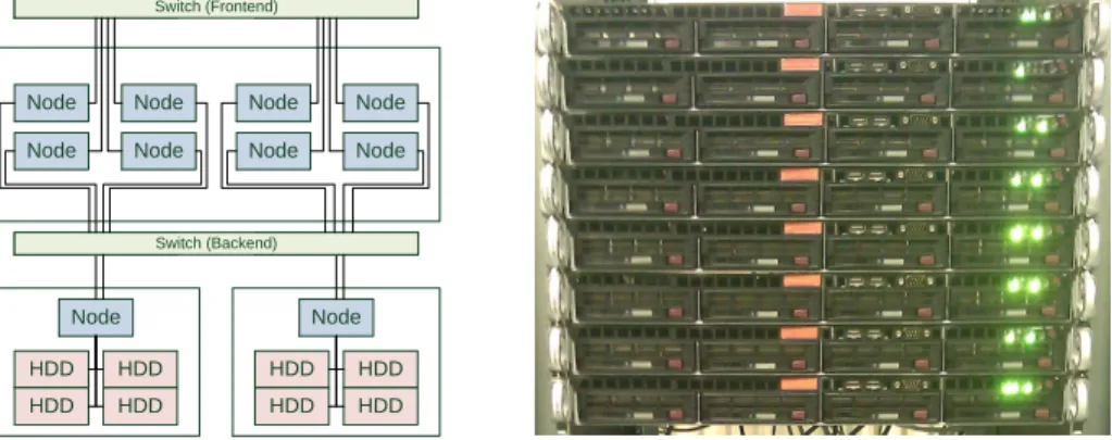
Our cluster currently consists of ten nodes with identical processors and main memory. Two nodes are equipped with four hard disks each to serve as DB storage. All nodes are interconnected by a Gigabit-Ethernet as depicted in Fig. 8. To minimize the energy footprint of each node, Intel Atom D510 light-weight
7
Such an extreme main-memory DB server would steadily consume 2.5 KW for each TB of main memory installed, no matter whether it is idle or working.
8
In this case, all coordination, query processing, and storage-related tasks have to be performed by this node.
HDD HDD HDD HDD Node HDD HDD HDD HDD Node Switch Switch Switch Switch Switch (Backend) Switch (Frontend) Node Node Node Node Node Node Node Node
Fig. 8:Physical cluster layout Fig. 9: Photo of the cluster
CPUs are used. In combination with the installed 2 GB of main memory and the mainboard, each node consumes less than 30 W in idle mode. The disks are designed for mobile use, so each disk consumes only 3 W . Our hardware isAmdahl-balanced, hence, processing power and data throughput are matched [20]. Still, a single node is not energy proportional as Table 2 shows. When idle, about 70% of the node’s peak power is consumed (see also Fig. 6). Although the single nodes are not energy proportional, the desired energy proportionality is approximated by load-dependent deactivation/reactivation of cluster nodes.
off suspend idle 100% CPU
1 disk 100% CPU 2 disks 100% CPU 4 disks Power Consumption [W] 3 3 29 32 35 41 % of peak 7% 8% 71% 78% 86% 100%
Table 2: Energy consumption of a single node
Dynamically powering nodes impacts all layers of database software. As a first step, we have analyzed the impact of node fluctuations forStorage Mapping, Query Processing andCluster Coordination.
5.2 Storage Mapping and Partitioning
Hard disks are one of the reasons, why common servers cannot be energy pro-portional, as explained in Sect. 2. They continuously consume energy to keep their platters spinning. Therefore, it would be a great opportunity for saving power, if unused disks could be switched off. If the related storage capacity is not needed right now, entire nodes could be powered down. Dynamically par-titioning data by their access frequencies may gain some improvements [21], but it is insufficient, because data on cold disks would have high access cost. In-stead, we propose a mechanism for dynamically consolidating data while keeping I/O performance agreements. The system’s storage can be scaled from energy
Table A
Partition A.1 Partition A.2
Disk 1
Table C
Partition C.1 Partition C.2
Disk 1 Disk 4
Partition
C.1.1 PartitionC.1.2 Partition C.2.1 Partition C.2.2
Disk 3 Disk 2 Table B Partition B.1 Disk 1 Disk 2 Partition B.2
Fig. 10:Storage partitioning schemes
efficiency requirements by consolidating data to as few disks as possible to high-performance needs by distributing data to more disks for faster parallel access. Fig. 10 shows examples of partitioning schemes. Table A is separated into two partitions that reside on a single disk. This is the most energy-efficient storage solution, because only a single disk needs to be powered. In turn, access per-formance is limited, as one disk can only achieve a certain number of IOPS. In contrast, table B is partitioned, too, but the partitions are distributed to sep-arate disks. Therefore, access to table B is up to two times faster than that to table A. At the same time, random IOPS should double compared to the first scheme, but energy consumption doubles as well. Finally,table C shows an even more distributed case, where data is distributed to four disks. While this raises the relative energy consumption of the data, access bandwidth and IOPS again are increased.
In these examples, the storage mapping resulted in a balanced tree of par-titions. WattDB will support even more flexible partitioning schemes. Hence, high-traffic areas of a table can be divided into finer grained partitions than rather cold areas – causing unbalanced partition trees. Management of a parti-tion subtree, e. g., either table C, partiparti-tion C.1, or partiparti-tion C.1.1 in Fig. 10, is delegated to a single node. By distributing a table to more nodes, the effective main-memory buffer for this table is increased.
5.3 Query Processing
By providing such an an energy-aware storage layer, query planning needs to consider the existing data distribution. A resulting query execution plan (QEP) has to reflect the data partitioning schemes and their assignment to nodes. As a consequence, subqueries can be formed to access partitions, process data, and emit intermediate results. Eventually, these results are consumed by a node which combines them to the final output and delivers it to the client. Fig. 11 sketches an example how this work assignment is achieved for a simple query. More sophisticated operations like distributed joins can be executed as well.
Our approach is considered fairly scalable, because partition management including buffering, locking, and recovery, consists of local tasks that scale with the number of nodes in the cluster. Still, a global transaction manager is needed to detect deadlocks in transactions spanning multiple nodes.
Table A
Partition ... Partition ... Partition ... Node 1 Table B Partition ... Partition ... Node 2 Table C Partition ... Partition ... Node 3 Master Node π( σ( A ) ) π( σ( C ) ) π( σ( A x B ) ) π( σ( A x C ) )
Fig. 11: Node assignment for query processing: an example
5.4 Cluster Coordination
Obviously, a centralized instance, called master, is needed for all coordination tasks. Cluster clients address a dedicated node as an entry point to submit their queries. Furthermore, it has to monitor and tune the performance of the cluster. Moreover, all tasks concerning allocation of new objects, housekeeping and reorganization on depraved storage structures, repartitioning after workload shifts, redistribution of responsibilities as an implication of cluster growth or shrinkage, etc. need centralized control. Therefore, we introduce a master node that will perform all these tasks. This node will also manage global deadlock detection and keep track of the energy consumption.
6
Conclusion and Future Work
We have sketched our main results of recent contributions concerning our flash-related research. At the device level, we have summarized performance behavior and energy efficiency of a spectrum of different SSD types and have discussed important consequences for DBMS processing. At the system level, we have com-pared performance and energy use of a number of flash-aware buffer management algorithms, when different classes of HDDs and SSDs were used as external stor-age. We could clearly verify the claim [16] that – within a single shared-nothing computing node – the most energy-efficient configuration is typically the highest performing one.
This observation guided our research endeavor towards energy-proportional computing applied to data management on new hardware to seriously observe energy saving – not only for peak loads, but also for low-load situations and even idle times. As a consequence, we designed WattDB, whose core components are currently implemented. In the future, we want to specialize WattDB towards differing directions to provide tailor-made support for the application classes OLTP, OLAP, and MapReduce.
References
1. Peter A. Boncz, Stefan Manegold, and Martin L. Kersten. Database Architecture Evolution: Mammals Flourished long before Dinosaurs became Extinct. InPVLDB 2(2), pages 1648–1653, 2009.
2. Greenplum. Driving the Future of Data Warehousing and Analytics.http://www. greenplum.com/, 2009.
3. VoltDB. Fast, Scalable, Open-Source SQL DBMS with ACID. http://voltdb. com/, 2010.
4. Hasso Plattner. SanssouciDB: An In-Memory Database for Processing Enterprise Workloads. InProc. BTW, LNI - P 180, pages 2–21, 2011.
5. Theo H¨arder, Karsten Schmidt, Yi Ou, and Sebastian B¨achle. Towards Flash Disk Use in Databases - Keeping Performance While Saving Energy? InProc. BTW, LNI - P 144, pages 167–186, 2009.
6. Volker Hudlet and Daniel Schall. SSD != SSD - An Empirical Study to Identify Common Properties and Type-specific Behavior. In Proc. BTW, LNI - P 180, pages 430–441, 2011.
7. Yi Ou, Theo H¨arder, and Daniel Schall. Performance and Power Evaluation of Flash-Aware Buffer Algorithms. InDEXA, LNCS 6261, pages 183–197, 2010. 8. Luc Bouganim, Bj¨orn Th´or J´onsson, and Philippe Bonnet. uFLIP: Understanding
Flash IO Patterns. InCIDR, 2009.
9. Goetz Graefe. The five-minute rule 20 years later (and how flash memory changes the rules). Commun. ACM, 52(7):48–59, 2009.
10. Daniel Schall, Volker Hudlet, and Theo H¨arder. Enhancing Energy Efficiency of Database Applications Using SSDs. InC3S2E, pages 1–9, 2010.
11. Wolfgang Effelsberg and Theo H¨arder. Principles of Database Buffer Management.
ACM TODS, 9(4):560–595, 12 1984.
12. Yi Ou, Theo H¨arder, and Peiquan Jin. CFDC: A Flash-Aware Buffer Management Algorithm for Database Systems. InADBIS, LNCS 6295, pages 435–449, 2010. 13. S. Park, D. Jung, et al. CFLRU: a Replacement Algorithm for Flash Memory. In
CASES, pages 234–241, 2006.
14. H. Jung, H. Shim, et al. LRU-WSR: Integration of LRU and Writes Sequence Reordering for Flash Memory. Trans. on Cons. Electr., 54(3):1215–1223, 2008. 15. D. Seo and D. Shin. Recently-evicted-first Buffer Replacement Policy for Flash
Storage Devices. Trans. on Cons. Electr., 54(3):1228–1235, 2008.
16. Dimitris Tsirogiannis, Stavros Harizopoulos, and Mehul A. Shah. Analyzing the Energy Efficiency of a Database Server. InSIGMOD, pages 231–242, 2010. 17. Luiz Andre Barroso and Urs H¨olzle. The Datacenter as a Computer: An
Introduc-tion to the Design of Warehouse-Scale Machines, Synthesis Lectures on Computer Architecture. Morgan & Claypool Publishers, 2009.
18. Susanne Albers. Energy-efficient Algorithms. Commun. ACM, 53(5):86–96, 2010. 19. Erhard Rahm. Evaluation of Closely Coupled Systems for High-Performance
Database Processing. InICDCS, pages 301–310, 1993.
20. Alexander S. Szalay, Gordon C. Bell, H. Howie Huang, Andreas Terzis, and Alainna White. Low-power Amdahl-balanced Blades for Data-intensive Comput-ing. SIGOPS Oper. Syst. Rev., 44.
21. Xiaodong Li, Zhenmin Li, Yuanyuan Zhou, and Sarita Adve. Performance-Directed Energy Management for Main Memory and Disks.Trans. Storage, 1:346–380, 2005.