i
ON MODELING THE SINGLE PERIOD SPARE PARTS DISTRIBUTION SYSTEM DESIGN PROBLEM BY MIXED INTEGER LINEAR
OPTIMIZATION
by
HAZAL ERCAN
Submitted to the Graduate School of Engineering and Natural Sciences
in partial fulfillment of the requirements for the degree of Master of Science
Sabancı University, July, 2019
iii
ACKNOWLEDGEMENTS
First and foremost, I would like to express my sincere gratitudes to Tübitak for giving me the opportunity of involving in the project 117M588.
I am heartily thankful to my supervisors Assoc. Prof. Dr. Güvenç Şahin and Asst. Prof. Dr. Tevhide Altekin for their patience, motivation, guidance and encouragement. I owe my deepest gratitudes to them, for not only inspring me every single day but also believing in me more than myself. Besides my supervisors, I would like to express my special appreciation to Assoc. Prof. Dr. Abdullah Daşçı and Asst. Prof. Dr. Ajinkya Tanksale for their expert advices and assistances.
Without my family, I would not be able to complete this thesis. Hence, I would like to thank my grandfather Salih Ercan and my grandmother Nafize Ercan for their endless support. Also, I am grateful to my father İskender Ercan and my mother Hale Özeren for always encouraging me throughout my thesis.
Last but not least, I would like to thank to my friends Lütfi Yiğit Erol, İmge Şipkan and Irmak Aktuğ for supporting me, believing in me and being there for me whenever I needed.
iv
ON MODELING THE SINGLE PERIOD SPARE PARTS DISTRIBUTION SYSTEM DESIGN PROBLEM BY MIXED INTEGER LINEAR
OPTIMIZATION
Hazal Ercan
Industrial Engineering, Master’s Thesis, 2019 Thesis Supervisor: Assoc. Prof. Dr. Güvenç Şahin
Thesis Co-Supervisor: Asst. Prof. Dr. Tevhide Altekin
Keywords: Distribution network, location-transportation problem, facility location, route generation, spare parts supply chain, post sale services
Abstract
Efficiency and effectiveness of spare parts logistics play a significant role in changing customers’ service levels. A company providing high quality after-sales support to their customers gains competitive advantages. To study a single period multi commodity spare parts distribution system design problem, we present a mathematical model in the form of a mixed integer linear programming problem formulation. The mathematical model incorporates facility location decisions and vehicle size selection as well as routing decisions. The problem formulation minimizes the total cost including opening and operating costs of the depots and transportation costs for the vehicles. In order to define and solve a realistic spare parts distribution system design problem, we use aggregation on the commodity flow data to reduce the size of the problem and generate the outbound distribution routes from the regional depots to the service points apriori to simplify the mathematical model. The main focus of this study is the apriori route generation; we aim to observe the impact of different route sets obtained by different heuristic methods. The solution quality and the computation time to solve the problems to optimality are used to compare the performance of the three routing heuristics.
v
TEK DÖNEMLİ YEDEK PARÇA DAĞITIM SİSTEMİ TASARIM PROBLEMİNİN KARIŞIK TAM SAYILI DOĞRUSAL OPTİMİZASYON İLE
MODELLENMESİ ÜZERİNE
Hazal Ercan
Endüstri Mühendisliği, Yüksek Lisans Tezi, 2019 Tez Danışmanı: Doç. Dr. Güvenç Şahin
Tez İkinci Danışmanı: Yard. Doç. Dr. Tevhide Altekin
Anahtar Kelimeler: Ağ tasarımı, yer-seçimi ulaştırma problemi, tesis yer seçimi,
rota oluşturma, yedek parça tedarik zinciri, satış sonrası hizmetleri
Özet
Yedek parça lojistik sistemlerinin etkinliği ve verimliliği müşterilerin hizmet düzeylerinin değiştirilmesinde önemli bir rol oynar. Yüksek kaliteli bir satış sonrası servisi vermesi firmaya rekabet üstünlüğü sağlar. Tek dönemli çok parçalı yedek parça dağıtım sistemi tasarım problemini çalışmak için, tesis yer seçimi ve araç büyüklüğü ile birlikte rotalama kararları da içeren tek amaç fonksiyonlu karmaşık tam sayılı doğrusal programlama problem gösterimi, depoların kurulum ve işletme maliyetleri ve araçların taşıma maliyetlerini içeren toplam maliyetini en küçükler. Gerçekçi bir yedek parça dağıtım sistemi probleminin tanımlanmasının ve çözülmesinin mümkün olması için, problemi küçültmek amacıyla ürün akış verisinde toplulaştırma ve matematiksel modelin kolaylaştırılması amacıyla servis noktalarına dağıtım rotalarının önceden yaratılması yoluna gidilmiştir. Çalışmamızın ana odağı rotaların önceden yaratılmasıdır. Farklı rotalama sezgiselleriyle yaratılan rota kümelerinin etkilerini gözlemlemeyi hedeflemekteyiz. Üç farklı rotalama sezgiselinin performansları, çözüm kalitesi ve optimal çözüm elde etmek için gerekli hesaplama zamanına bakılarak karşılaştırılacaktır.
vi
TABLE OF CONTENTS
1. Introduction ... 1
2. Spare Parts Distribution System Design ... 3
2.1. Literature Review ... 3
2.2. Problem Definition and Mathematical Model ... 7
2.2.1. Problem Definition ... 7
2.2.2. Mathematical Model ... 10
3. Part Aggregation and Route Generation ... 14
3.1. Part Aggregation ... 14
3.1.1. Supplier Based Aggregation ... 15
3.1.2. Part Based Aggregation... 15
3.1.3. Code Based Aggregation... 15
3.2. Route Generation ... 16 3.2.1. Literature Review ... 16 3.2.2. Heuristic Methods ... 18 4. Computational Results ... 24 4.1. Experimental Design ... 24 4.2. Computational Experiments ... 26
4.2.1. Summary of Generated Routes ... 26
4.2.2. Results of Computational Experiments ... 31
4.2.2.1. Results for an Example Problem ... 31
4.2.2.2. Overall Results ... 36
5. Conclusion ... 45
REFERENCES ... 47
APPENDIX A: Detailed Information on Routes Generated by ENS Heuristic for problem Instance 1 in the set with 30 Service Points and 10 Regional Depots ... 52
APPENDIX B: Detailed Information on Routes Generated by NN Heuristic for problem Instance 1 in the set with 30 Service Points and 10 Regional Depots ... 55
APPENDIX C: Detailed Information on Routes Generated by SAV Heuristic for problem Instance 1 in the set with 30 Service Points and 10 Regional Depots ... 56
APPENDIX D: Service Points – Parts Assignment for ENS Heuristic ... 58
APPENDIX E: Service Points – Parts Assignment for NN Heuristic ... 59
APPENDIX F: Service Points – Parts Assignment for SAV Heuristic ... 60
vii
LIST OF TABLES
Table 2.1 The differences between our study and most similar studies ... 6
Table 3.1 The differences between our study and other route generation studies .... 19
Table 4.1 Inbound transportation costs used ... 26
Table 4.2 Outbound transportation costs used ... 26
Table 4.3 Summary of ENS generated routes ... 27
Table 4.4 Summary of NN generated routes ... 27
Table 4.5 Summary of savings algorithm generated routes ... 27
Table 4.6 Number of routes and number of variables of the three heuristics ... 29
Table 4.7 Number of binary variables and number of constraints of the three heuristics ... 30
Table 4.8 Number of common routes between heuristics ... 31
Table 4.9 Total cost breakdown of the solution using ENS algorithm’s routes ... 32
Table 4.10 Regional depots and IB shipment details using ENS algorithm’s routes ... 32
Table 4.11 Selected routes and OB shipment details using ENS algorithm’s routes ... 33
Table 4.12 Total cost breakdown of the solution using NN algorithm’s routes ... 34
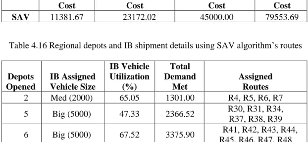
Table 4.13 Regional depots and IB shipment details using NN algorithm’s routes . 34 Table 4.14 Selected routes and OB shipment details using NN algorithm’s routes . 34 Table 4.15 Total cost breakdown of the solution using SAV algorithm’s routes ... 35
Table 4.16 Regional depots and IB shipment details using SAV algorithm’s routes ... 35
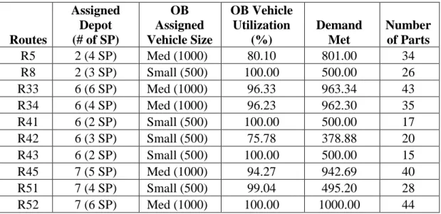
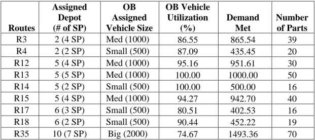
Table 4.17 Selected routes and OB shipment details using SAV algorithm’s routes ... 35
Table 4.18 Number of vehicles of three heuristics ... 36
Table 4.19 Objective function values and bounds obtained using the three route sets ... 37
Table 4.20 Number of best solutions found by each route generation heuristic ... 38
Table 4.21 Average of percentage differences with the best heuristic ... 38
Table 4.22 Average of the cost componets according to the problem sizes and heuristics ... 40
Table 4.23 Average of the number of vehicles used ... 40
Table 4.24 Average of inbound and outbound vehicle utilizations ... 40
Table 4.25 Average number of service points with multiple routes ... 41
Table 4.26 Average number of selected routes ... 41
Table 4.27 Average number of regional depots opened ... 42
Table 4.28 Percentage gaps and CPU times of each route generation heuristic ... 43
viii
LIST OF FIGURES
Figure 2.1 Proposed spare parts distribution system ... 10 Figure 2.2 Demonstration of two regional depots and two routes assigned to each . 13 Figure 4.1 Instance 1 of 30 service points and 10 regional depots ... 25
1
1. Introduction
After-sales service refers to the processes that are undertaken by the company for the care of the customers after they purchase a good or a service. In most manufacturing companies, after-sales service has a critical role since it increases profitability, customer satisfaction and
customer retention potential (Saccani et al. 2007; Alexander et al. 2002). The profit margins
for initial sales of a company is approximately 10%, whereas for after-sales services it is
three times larger (Murthy et al. 2004). In some of the industries such as automobiles, white
goods and information technology, the after-sales service market sizes are up to five times larger than the equipment businesses (Bundschuh and Dezvane 2003; Cohen 2006). Therefore, the companies that provide high quality after-sales support to their customers can gain also competitive advantage in the market (Cohen 2006).
We investigate a spare parts distribution system design problem which is inspired from the case of a white household goods manufacturer in Turkey. The household appliances company engages in the production as well as the marketing of the durable goods, components and multiple product parts. We consider an after-sales services supply chain that consists of a distribution center, regional depots and service points representing authorized repair vendors. The inbound transportation of the spare parts from the distribution center to the regional depot can be done using different vehicles. Similarly, the outbound transportation from regional depots to the service points can be done utilizing different vehicles and routes. Our aim is to determine intermediate regional depot locations and assign service points to the regional depots while considering other real life aspects such as routing decisions and selecting vehicle sizes. While minimizing the total cost of the network, both strategic (regional depot location determination) and tactical (route and vehicle size selection) level decisions are included. Therefore, this spare parts distribution system design problem can be associated with location-routing and location-transportation problems.
In order to design the after-sales spare parts distribution system, a static single period multi-commodity system design problem is defined and a mixed integer linear mathematical model is developed. The mathematical programming formulation’s objective function is based on minimizing the total cost and includes the opening and operating costs of the
2
regional depots and both inbound and outbound transportation costs. The proposed mathematical formulation is solved using a commercial solver for instances of four different problem sizes. However, route optimization is beyond the scope of our study. Alternative routes are generated using the savings algorithm, nearest neighbor algorithm and expanded neighbor search algorithm in order to analyze the impact of given route sets. Our contributions can be summarized as follows:
• We define a realistic new spare parts distribution system design problem that
incorporates route and vehicle size selection decisions. Hence, staircase cost structures are used to represent different vehicle sizes for inbound and outbound transportations.
• We develop the mathematical model for the spare parts distribution system design
problem.
• Three different heuristics are used to provide different route sets as input. Based on
the analysis of the given routes of the white household goods manufacturer in Turkey, we adopt two algorithms from the literature and propose an extension.
• Similarly, the determination of the number of spare parts to include in our
multi-commodity problem is based on aggregating more than 40,000 spare parts of the same manufacturer.
• We demonstrate the impact of the given route sets on the solution quality and
computation time.
The remainder of this thesis is organized as follows: Chapter 2 consists of a literature review, problem definition and the proposed mathematical model. Demand aggregation strategies and route generation heuristics are given in Chapter 3. In Chapter 4, we present the computational results. Finally, we conclude with the main findings in Chapter 5.
3
2. Spare Parts Distribution System Design
In this chapter, we first summarize the literature of after-sales logistics systems. Then, we continue with comparing our study with the most similar studies. We also present our problem definition and underline the distinguishing features of our study, which involve the inclusion of vehicle size (type) selection and route selection. Finally, we present our mixed integer linear programming model.
2.1. Literature Review
After-sales logistics systems provide spare parts, maintenance and repair services to their
customers (Cohen et al. 1997). Typically, the profit margin for initial sale products is
approximately 10% in contrast to 30% on the post-sale service products (Murthy et al.
2004). For a typical manufacturing company, after-sales services and parts can contribute up to 50% of all profits (Dennis and Kambil 2003). After-sales activities are one of the most important types of sources of income, which provide a competitive advantage to the
producers (Saccani et al. 2007; Cohen et al. 2006).
Hertz et al. (2012) suggest that planning problems of the traditional supply chains have been
investigated for decades but they are newly investigated for the after-sales networks. In the literature, spare part distribution systems are claimed to differ from the production distribution systems due to various factors such as large number of parts, high prices, short lead times, uncertainty in demand, multiple classes of services and the requirement to meet
service requests in a timely manner (Cohen et al. 1999; Cohen et al. 2006; Huiskonen 2001).
Our system is considered as a spare part distribution system rather than a production-distribution system due to the various differentiations such as large number of spare parts, unpredictable demands, heterogeneous product portfolio, quick response needs of services.
The variety of the operational control characteristics of the spare parts have a huge impact on network structure, positioning of materials, responsibility of control and control principles. Operational control characteristics such as criticality, specificity, value of parts and demand pattern are evaluated due to their impact on the plan and the design of the network logistics system (Huiskonen 2001). Due to the difference between the operational control characteristics, spare part distribution systems are prominently different than the traditional production distribution networks.
4
Hu et al. (2018) provide a review of operational research models used in spare parts management. However, their analysis on optimization techniques used has excluded the studies on the design of distribution networks for spare parts. The literature on distribution network design for spare part supply chains is somehow very limited.
Murthy et al. (2004) summarize product warranty logistics literature. Bacchetti and Saccani
(2012) investigate theoretical contributions about spare parts classification and demand
forecasting for stock control. Cohen et al. (1997) present a comparison analysis between
high value products and technologically complicated products. The literature of supply chain spare part distribution design also involves empirical studies which are from different
industries. For instance, Saccani et al. (2006) examine household appliances, information
technologies, consumer electronics and automotive industries, whereas Saccani et al. (2007)
investigate durable consumer goods industry. In addition to the industry based studies, there are also studies on the improvement of after-sales services of particular production companies such as:
• IBM (Cohen et al. 1990; Jalil et al. 2011)
• Teradyne (Cohen et al. 1999)
• Saturn (Cohen et al. 2000)
• Heavy duty equipment producer (Persson and Saccani, 2009)
• Digital cinema projector producer (Landrieux and Vandaele, 2012)
• High valued fixed asset producer (Driessen et al. 2015)
• Household appliances manufacturer (Altekin et al. 2017)
Among the literature that involves the design of the after-sales logistics networks, in order to determine the locations of the facilities and determine the flow among those facilities,
quantitative methods are proposed by Persson and Saccani (2009), Wu et al. (2011), Jalil et
al. (2011) and Landrieux and Vandaele (2012). Persson and Saccani (2009) analyze the
allocation of parts and suppliers for a second European warehouse through a simulation model. This study focuses on evaluating possible choices of spare part inventory locations, as well as analyzing the classification criteria of the spare parts that determine the inventory
policy to be used. The study of Wu et al. (2011) involves decisions such as logistic network
design, service point selection and transportation mode selection in order to solve a
5
spare parts logistics through an installed based real-life case. Also, the data errors of their installed base case are identified and the effects of these errors on the performance of spare parts planning are determined. Landrieux and Vandaele (2012) develop a model for the distribution of the spare parts. Under four different scenarios, solutions of the spare parts inventory management and facility location problem are evaluated based on the total cost and facility assignment of the customers.
Altekin et al. (2017) have formulated the multi-level, multi-commodity spare parts
distribution network of a household appliances manufacturer in Turkey. The large-scale problem consisting of more than 40,000 spare parts and nearly 700 facility locations has been transformed into a realistic smaller scale problem. The proposed mixed integer programming model minimizes the total cost of the network, determines the locations of the facilities, assigns the service points to the selected facilities and selects transportation modes. For eight scenarios representing different network configurations, optimal solutions obtained using a commercial solver are evaluated.
Our study is inspired by the spare parts distribution system design problem in Altekin et al.
(2017). Two of their scenarios included 73 routes given by the company for the outbound shipments of the spare parts from regional depots to service points. Hence, we include the selection of route decisions for outbound shipments. We also incorporate vehicle size selection decisions for both the inbound and outbound transportations using a staircase cost
structure. Stochastic multi-period location-transportation problem in Klibi et al. (2010) also
consists of determining vehicle sizes and routes to be used from given alternative routes in addition to facility location decisions. Their objective function is maximizing profit and they exclude inbound transportations.
We develop a mathematical model that will be solved by a commercial solver. The main decisions include the number and location of regional depots, number and size of inbound and outbound vehicles, selection of routes and transportation quantities. Our objective includes understanding the effect of the given routes on the solution time and quality.
Weak lower bounds may rise because of the staircase cost structures (Croxton et al. 2003a)
which also lead to create weak formulations in some of the transportation problems (Croxton et al. 2003b; Harks et al. 2014). Staircase cost structures arise and cause computational challenges not only in transportation problems but also in location and capacity problems
6
(Holmberg 1994; Holmberg and Ling 1997; Correia and Captivo 2003; Correia and Captivo
2006; Correie et al. 2010), design problems (Mahey et al. 2001; Christensen 2013), and
supplier selection problems (Andrade-Pineda et al. 2017).
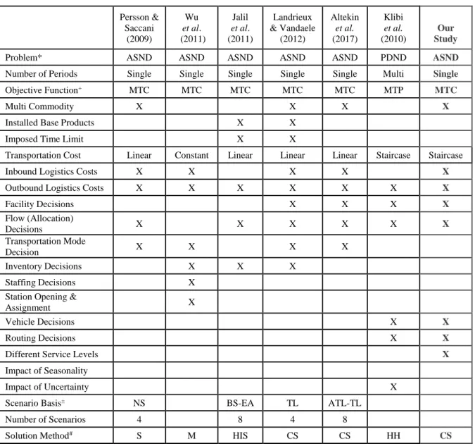
The differences between our study and most similar studies are given in Table 2.1. Our objective is to provide a realistic spare parts distribution system design problem definition, to formulate it as a mixed integer linear programming model, to solve it using a commercial solver and to demonstrate the impact of the given routes on solution time and quality.
Table 2.1 The differences between our study and most similar studies
Persson & Saccani (2009) Wu et al. (2011) Jalil et al. (2011) Landrieux & Vandaele (2012) Altekin etal. (2017) Klibi et al. (2010) Our Study
Problem* ASND ASND ASND ASND ASND PDND ASND
Number of Periods Single Single Single Single Single Multi Single
Objective Function+ MTC MTC MTC MTC MTC MTP MTC
Multi Commodity X X X X
Installed Base Products X X
Imposed Time Limit X X
Transportation Cost Linear Constant Linear Linear Linear Staircase Staircase
Inbound Logistics Costs X X X X X
Outbound Logistics Costs X X X X X X X
Facility Decisions X X X X Flow (Allocation) Decisions X X X X X X Transportation Mode Decision X X X X Inventory Decisions X X X Staffing Decisions X
Station Opening &
Assignment X
Vehicle Decisions X X
Routing Decisions X X
Different Service Levels X
Impact of Seasonality
Impact of Uncertainty X
Scenario Basis± NS BS-EA TL ATL-TL
Number of Scenarios 4 8 4 8
Solution Method# S M HIS CS CS HH CS
* ASND: After-Sales Network Design; PDND: Production Distribution Network Design. + MTC: Minimize Total Cost; MTP: Maximize Total Profit.
± NS: Number of suppliers served by new warehouse; BS-EA: Installed base size and error accuracy;
TL: Time Limit; ATL: Allowed transportation links.
# S: Simulation; M: Metaheuristics; IHS: In-house solver; CS: Commercial solver; HH: Hierarchical heuristics (tabu
7
2.2. Problem Definition and Mathematical Model
2.2.1. Problem Definition
This study is motivated by the purpose of introducing a new spare parts distribution system design problem through the inclusion of route selection for outbound shipments and vehicle size selection for both inbound to and outbound transportations from the regional depots. After-sales service systems provide an interface between the firms and customers in order to respond to customers’ maintenance and repair requests. Through its regional depots and distribution systems, after-sales service systems are responsible of transporting of a high variety of parts that are procured from various suppliers to a high variety of service points. Although there is a variety of decisions involved in establishing and operating such systems, we focus on finding the locations of the regional depots from which the parts are sent to the service points. This higher level decision profoundly affect impact on the performance/effectiveness of the system. As well as specifying the location of the regional depots, we also consider other operational issues such as spare part flows, and selection of routes as well as sizes of vehicles for both inbound and outbound transportations.
We are inspired by the spare parts distribution system of a household appliance manufacturer in Turkey, which was studied previously in Aylı (2015). Although it is known that the responsiveness to the customers has an immense importance in terms of the
competition in the market, in Altekin et al. (2017), it is noted that the spare parts service
systems in Turkey are managed in a cost-oriented manner. The reviewed literature on spare parts distribution system design demonstrates the available content is limited. Therefore, in both practice and academia, more realistic approaches are necessary in order to design more effective and efficient spare parts distribution systems. Next, we will present the details on two features that differentiate our study from the available studies and enable the design of efficient and effective spare parts distribution systems.
8 Route Selection Decisions
The first extension on Altekin et al. (2017), is the inclusion of alternative approaches of
route formation where a route is defined as a set of service points to be visited by the vehicle. Even though route optimization is beyond the scope of this study, alternative routes will be
constructed for the given service points. In Altekin et al. (2017), 73 given routes are used to
cover all of the 531 service points. The routes given by the company and used in Altekin et
al. (2017) are examined and the following observations are made:
• All of the 531 service points are covered by a single regional depot (i.e.
single-sourcing is enforced).
• Every service point is assigned exactly to one route.
• It is not certain if the company includes the vehicle size constraint while constructing
the 73 routes.
• We think factors such as maximum driving speed, daily limit on driving hours,
service time associated with unloading and delivering the spare parts have been used in addition to classifications based on congestion of the locations of the service points.
Altekin et al. (2017) have solved the problem with a more limited approach, where delivery
routes are pre-specified. In our study, in order to observe the effect of the given alternative routes on the results of the mathematical model, alternative routes will be generated by three different algorithms.
Alternative Vehicle Types
We extend the work and the contribution in Aylı (2015) and Altekin et al. (2017) by also
including the selection of vehicle sizes. The vehicle size dimension consists of three options: small, medium and large. As the volume of the vehicle increases, the fixed cost of using that truck also increases. The motivation behind this extension is the opportunity of creating a possible decrease on the total cost.
The solution to a spare part system design problem should satisfy the demands of the service points from the distribution center through regional depots. There are some assumptions that
9
define the structure of the spare part distribution system design problem such as the following:
• There is only one distribution center in the system.
• There is no restriction on the number of opened and operated regional depots and
the corresponding costs of opening and operating those regional depots are given.
• There is no restriction on the capacity of regional depots.
• The locations of the service points, regional depots and distribution center are given.
• The demands of the service points for different parts are known.
• The transportation costs are defined with an increasing staircase cost function.
• The transportation from the regional depots to the service points will be through the
given routes.
• A service point can be assigned to more than one route. Thus, a service point can
also be covered by more than one regional depot.
• The given routes are generated for each regional depot. Hence, the same route might
be independently generated for more than one regional depot.
• Determining the inventory levels of the spare parts of the distribution center and the
regional depots are beyond the scope of this study.
Figure 2.1. demonstrates the proposed spare parts distribution system. The main aim of the spare part distribution system design problem is to minimize the total cost while the main decisions are summarized as follows:
• the number and location of the regional depots to open,
• the amount of spare parts transported from distribution center to the regional depots,
• the route and the amount of spare parts to be transported from the regional depots to
the service points,
• the size of the vehicles to be used for inbound transportation,
10
Figure 2.1 Proposed spare parts distribution system
2.2.2. Mathematical Model
In order to depict the mathematical model developed for the spare part distribution system design problem, we first present the sets, the parameters and the decision variables.
Sets:
𝐼: alternative regional depots
𝐽: service points
𝑃: part families
𝑅: all routes from potential regional depot locations to service points
𝑅𝑖: set of routes that are assigned to regional depot i 𝑅𝑗: set of routes that contain service point j
𝐽𝑟: service points covered in route r
𝑘 ∈ 𝐾𝑟: volume breaks (0 < 𝑄𝑟1 < 𝑄𝑟2 < . . . ) for outbound transportation cost
function for route r
𝑘 ∈ 𝐾𝑖′: volume breaks (0 < 𝑄′𝑖1 < 𝑄′𝑖2 < . . . ) for inbound transportation cost
11 Parameters:
𝐷𝑗𝑝: demand of service point j for part p (in terms of volume)
𝑓𝑖: fixed cost of opening a regional depot at location i
𝑐𝑟𝑘: outbound transportation cost for volumes less than or equal to Qrk on route r
𝑐′𝑖𝑘: inbound transportation cost for volumes less than or equal to 𝑄′𝑖𝑘 from
distribution center to the regional depot i
Decision variables:
𝑥𝑗𝑝𝑟: Amount (volume) of part 𝑝 delivered to service point 𝑗 through route r
𝑦𝑖: {
1, if a regional depot is opened at location 𝑖
0, otherwise
𝑣𝑟𝑘: {
1, if transportation option k is utilized on route r
0, otherwise
𝑤𝑖𝑘:
{
1, if transportation option 𝑘 is utilized from distribution center to regional
depot 𝑖
0, otherwise
Accordingly, the mathematical model can be presented as follows:
Minimize ∑ 𝑓𝑖 𝑖∈𝐼 𝑦𝑖 + ∑ ∑ 𝑐𝑟𝑘 𝑘∈𝐾𝑟 𝑣𝑟𝑘 𝑟∈𝑅 + ∑ ∑ 𝑐′𝑖𝑘 𝑘∈𝐾𝑖′ 𝑤𝑖𝑘 𝑖∈𝐼 (1) subject to ∑ 𝑥𝑗𝑝𝑟 𝑟∈𝑅𝑗 = 𝐷𝑗𝑝 , ∀ (𝑗, 𝑝) ∈ (𝐽, 𝑃), (2) ∑ ∑ 𝑥𝑗𝑝𝑟 𝑝∈𝑃 𝑗∈𝐽𝑟 ≤ ∑ 𝑄𝑟𝑘 𝑘∈𝐾𝑟 𝑣𝑟𝑘 , ∀ 𝑟 ∈ 𝑅, (3) ∑ ∑ ∑ 𝑥𝑗𝑝𝑟 𝑝∈𝑃 𝑗∈𝐽𝑟 𝑟∈𝑅𝑖 ≤ ∑ 𝑄′𝑖𝑘 𝑘∈𝐾𝑖′ 𝑤𝑖𝑘 , ∀ 𝑖 ∈ 𝐼, (4) ∑ 𝑣𝑟𝑘 𝑘∈𝐾𝑟 ≤ 𝑦𝑖 , ∀ (𝑖, 𝑟) ∈ (𝐼, 𝑅𝑖), (5) ∑ 𝑤𝑖𝑘 𝑘∈𝐾𝑖′ ≤ 𝑦𝑖 , ∀ 𝑖 ∈ 𝐼 , (6) 𝑥𝑗𝑝𝑟 ≥ 0 , ∀ (𝑗, 𝑝, 𝑟) ∈ (𝐽, 𝑃, 𝑅𝑗), (7) 𝑦𝑖 ∈ {0,1} ∀ 𝑖 ∈ 𝐼, (8)
12
𝑣𝑟𝑘 ∈ {0,1} ∀ (𝑟, 𝑘) ∈ (𝑅, 𝐾𝑟), (9) 𝑤𝑖𝑘 ∈ {0,1} ∀ (𝑖, 𝑘) ∈ (𝐼, 𝐾𝑖). (10)
The objective function (1) minimizes the total cost of the network and consists of fixed opening and operating costs of the regional depots, inbound transportation costs from DC
to regional depots as well as outbound transportation costs from regional depots to the
service points. Constraint (2) ensures that the demand of each service point is satisfied for all part families. Constraints (3) and (4) are the outbound and inbound flow capacity constraints that warrant the transportation capacities for the deliveries depending on the selected vehicle size. The outbound flow capacity constraint includes the delivery from the regional depots to the service points where the inbound capacity constraint includes the delivery from the DC to the regional depots. Constraints (5) and (6) are the outbound and inbound truck selection constraints ensuring that only open regional depots are used for the possible deliveries and also that one volume break is used during these deliveries representing the vehicle size selection decision. Finally, constraints (7), (8), (9) and (10) are the domain constraints for the decision variables.
The provided mathematical model is also strengthened with the addition of the following three valid inequalities.
∑ ∑ 𝑣𝑟𝑘 𝑘∈𝐾𝑟 𝑟∈𝑅𝑗 ≥ 1, ∀𝑗 ∈ 𝐽+ = {𝑗 ∈ 𝐽: 𝐷𝑗𝑝 > 0, ∃𝑝 ∈ 𝑃}, (11) ∑ ∑ 𝑣𝑟𝑘 𝑘∈𝐾𝑟 𝑟∈𝑅𝑖 ≥ 𝑦𝑖 , ∀ 𝑖 ∈ 𝐼, (12) ∑ 𝑤𝑖𝑘 𝑘∈𝐾𝑖′ ≥ 𝑦𝑖 , ∀ 𝑖 ∈ 𝐼. (13)
Valid inequality (11) ensures that a service point with any positive demand for the spare
parts, will visited. If depot i is opened, valid inequalities (12) and (13) ensure the usage of
inbound and outbound vehicles.
A solution to this static problem yields a set of opened regional depots, number and sizes of inbound vehicles to the regional depots from the distribution center, a set of selected routes, sizes of vehicles used on the selected routes for the outbound vehicles to the service points and quantities of the transported spare parts. Figure 2 demonstrates a simple solution with
13
two regional depots and two routes assigned to each. A service point can be assigned to more than one depot. Moreover, a service point can be served using two different routes. Thus, it can be underlined that our model provides flexibility by not enforcing single
sourcing which was the case in Altekin et al. (2017).
14 3. Part Aggregation and Route Generation
In this chapter, alternative aggregation strategies are implemented on the past data regarding the commodity flows in the system obtained from the household appliances manufacturer
in Altekin et al. (2017) in order to decrease the number of part families to be included so as
to reduce the problem size with respect to type of commodities. After determining the number of part families, we focus on the route generation and provide both a brief review of the relevant literature and the details of the three heuristics used.
3.1. Part Aggregation
In large-scale distribution system design problems, an important issue is associated with the aggregation of commodity flow data as this process has direct impact on the problem size
due to the number of parts included in the problem. Altekin et al. (2017)’s multi-level
facility location problem for spare parts distribution system design studied an aggregation based on the suppliers. First, each supplier was assumed to provide one aggregated spare part with a demand equal to total demand (in volume) of all parts from the same supplier. Then, 93 supplier-based items were reduced to 16 using Pareto analysis. In our study, one
of the main purposes is to develop alternative aggregation approaches to those in Altekin et
al. (2017) in which more than 40,000 individual spare parts exist.
In the multi-level facility location problem representing our spare parts distribution system we have studied alternative aggregation strategies in order to determine the number of parts to be included. Among 1,801 spare parts, 94 parts have incomplete information. Hence, the aggregation strategies are applied to the remaining 1,707 spare parts whose volume and demand information are available and those that have demand greater than 1,000 units. Accordingly, the following three aggregation strategies are proposed:
• Supplier based strategies
• Part based strategies
15
3.1.1. Supplier Based Aggregation
We present two different supplier-based aggregation strategies. In the first one, each supplier is treated as an individual part family. Since there are 49 suppliers of those 1,707 parts, we have 49 different part families. Hence, for each part family, the parts are provided by the same supplier. Then, the number of parts supplied by these 49 suppliers are determined. If the number of parts that are supplied by the same supplier is less than ten, such suppliers are merged under one fictive supplier. With this approach, 16 part families are obtained.
In the second one, the suppliers that provide more than ten parts are investigated individually. For each supplier, the volumetric demand of all the parts they provide are sorted in an increasing order. Then a Pareto-based analysis is used to construct part families. Hence, instead of taking each supplier as a single part family, this strategy facilitates inclusion of multiple part families from big suppliers. For all of the suppliers that supply
less than ten parts, the fictive supplier is assumed to provide a single part.
3.1.2. Part Based Aggregation
The corresponding volumetric demand information of every single part (independent from their supplier) are identified and sorted. Again, Pareto-based analysis is used to construct the part families. The same approach can be implemented by either using only the volume or only demand data.
3.1.3. Code Based Aggregation
In this strategy, part families are constructed by using only their code number. The first number of the part code and the number of digits in the code number are used for the identification of part families. Then, each part family (13) is investigated based on volumetric demand information and sorted accordingly. Again Pareto-based analysis of each part family is used to further divide it into several new part families. The number of part families that are constructed as a result of this strategy is 42. In order to further decrease the number of the part families, the summations of the volumetric demand values of each part family (42) are sorted. Application of similar Pareto-based analysis has yielded 7 part families.
16
As a result of the analysis of these three different part aggregation strategies, the obtained number of the part families ranges between 7 and 16. In the scope of our spare part distribution system design problem, we eventually study problems with 10 part families; this is not only consistent with the results of the aggregation strategies we test but also compatible with real life data of our example.
3.2. Route Generation
The efficiency and effectiveness of the proposed mathematical model depends on the given set of routes and involves a trade-off: providing a high number of routes increases both the solution time and quality while providing few number of routes decreases the solution time and might lead to inferior solutions in terms of the total cost. On the other hand, for big instances solutions with lower optimality gaps might be obtained when fewer routes are given. Hence, we study three different algorithms to generate routes to investigate their impact on the solution quality for the spare parts distribution system design problem and required computational effort.
We first provide a brief overview of literature on the facility location problem that includes routing decisions, and then, present the three alternative heuristic methods to generate routes in detail.
3.2.1. Literature Review
In the literature, production distribution system design problem focuses on two main issues which are determination of the facility locations and generation of the routes.
Elson (1972) presents the first mathematical modelling of the facility location problem which shows that mixed integer programming can be applicable to the solution of certain site location problems. Geoffrion and Graves (1974) study the optimal locations of distribution facilities between plants and customers. Solution technique of that distribution system design problem is based on Bender’s decomposition. They apply their solution approach to a real problem of a food company. In addition to their consideration of facility opening costs, Geoffrion and Graves (1974) propose the first route oriented formulation. With a similar model to Geoffrion and Graves (1974), Pirkul and Jayaraman (1996) focus on a plant and warehouse location problem where they employ Langrangian relaxation.
17
Most of the facility location problems consider that transportation alternatives are planned and uncapacitated. Moreover, majority of the studies assume that the approximate transportation cost between two points is a simple linear function of the amount transported. However, there are some studies that avoid these assumptions by including transportation
capacity constraints (Yılmaz and Çatay (2006); Li et al. (2009); Carle et al. (2012) and
Meisel et al. (2016)), transportation mode decisions (Carle et al. (2012); Sadjady and
Davoudpour (2012) and Meisel et al. (2016)) and vehicle type decision (Eskigun et al.
(2005) and Validi et al. (2015)).
Even though, many studies in the literature discuss issues such as capacitated transportation alternatives, transportation mode selection and vehicle type selection, these studies assume direct transportation between the facilities and customers instead of milk-run logistics structure. Milk-run is a delivery method in which a vehicle visits each supplier on a fixed route in order to meet customer needs instead of visiting each supplier separately. In their study, Brar and Saini (2011) state that milk-run system results in transportation cost reduction and vehicle utility maximization. Although milk-run is a procurement method that uses routing to deliver goods to the consumers, it excludes routing decisions. The first combination of facility location decisions and routing decisions are discussed in Maranzana (1964). In the 1990s, the number of studies that combine location-transportation problem
with routing has increased and include: Min et al. (1998), Nagy and Salhi (2007), Lopes et
al. (2013), Prodhon and Prins (2014) and Drexl and Schneider (2015).
Bookbinder and Reece (1988) enhance the study of Geoffrion and Graves (1974) by adding routing decisions and vehicle size selection. In location-routing literature, the most similar study to ours is the study of Bookbinder and Reece (1988) since it also focuses on a two-stage distribution system in which the transportation from factories to consumers is done via depots.
Jacobsen and Madsen (1980) and Madsen (1983) discuss the two-stage location-routing problem for the first time in the literature. Following Madsen (1983), Ambrosino and
Scutella (2005) and Ambrosino et al. (2009) develop models that combine distribution
system design and detailed routing. Through their study of two-stage location-routing problem, Lin and Lei (2009) categorize clients as big clients and other clients and only include the big clients to the first-level routing.
18
Route optimization is beyond the scope of our study. Hence, route optimization is included neither at the first-level nor at the second-level of the spare parts distribution system. Furthermore, routing decisions are not included in the first-level our system which involves transportation from DC to the regional depots. Therefore, the main focus of the first-level is determining the locations of the regional depots and inbound vehicle type size selection. However, the routing decisions in the second-level involve selecting the routes from opened regional depots to the service points. Consequently, our study is not a location-routing problem; route planning decisions are made heuristically by giving a set of generated routes as input. Similar to Nagy and Salhi (2007), our study is associated with location-transportation problem.
In our study, we aim to solve a spare part distribution system design problem inspired from a real-life household appliances manufacturer by using the proposed mathematical model.
Recall that Klibi et al. (2010) was also incorporating routing decisions in a similar approach
to ours. In order to generate the alternative routes, we reviewed the routing literature for
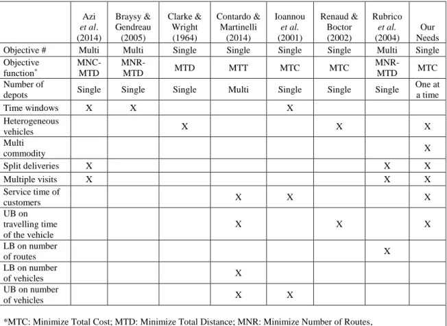
existing routing heuristics which can be applied to our study such as Azi et al. (2014),
Braysy and Gendreau (2005), Clarke and Wright (1964), Contardo and Martinelli (2014),
Ioannou et al. (2001), Renaud and Boctor (2002) and Rubrico et al. (2004). Table 3.1
presents a comparison of these studies and the factors that must considered while generating routes for our problem. After assessing the relevant studies in terms of various features that are needed in our study, we have found Clarke and Wright (1964)’s savings algorithm along with the nearest neighbor algorithm applicable for heuristically generating good routes.
3.2.2. Heuristic Methods
In this study, alternative routes will be generated by using three heuristics in order to facilitate route planning decisions of the proposed mathematical model. The two of the heuristics are modifications of existing heuristics which are Clarke and Wright (1964)’s savings algorithm and nearest neighbor algorithm. Although the three algorithms differ from each other, they have common points, such as creating a candidate service point list for each depot. For a service point to be included in the candidate service point list of a regional depot, the distance from the service point to the corresponding depot should be less than or equal to a given threshold value; we call this value as the routing diameter.
19
Recall that in our study a route defines only the set of service points visited. Therefore, in all the three algorithms, for each regional depot, if two of the generated routes cover the same service points (regardless of their order) they are treated as the same route. Hence, our algorithm excludes the duplicates of the existing routes.
Table 3.1 The differences between our study and other route generation studies
Azi et al. (2014) Braysy & Gendreau (2005) Clarke & Wright (1964) Contardo & Martinelli (2014) Ioannou et al. (2001) Renaud & Boctor (2002) Rubrico et al. (2004) Our Needs Objective # Multi Multi Single Single Single Single Multi Single Objective function* MNC- MTD MNR- MTD MTD MTT MTC MTC MNR- MTD MTC Number of
depots Single Single Single Multi Single Single Single
One at a time Time windows X X X Heterogeneous vehicles X X X Multi commodity X Split deliveries X X X Multiple visits X X X Service time of customers X X X UB on travelling time of the vehicle X X X LB on number of routes X LB on number of vehicles X UB on number of vehicles X X
*MTC: Minimize Total Cost; MTD: Minimize Total Distance; MNR: Minimize Number of Routes, MNC: Minimize Number of Served Customers; MTT: Minimize Total Time
Savings Algorithm
One of the well-known and widely used route construction heuristics for routing problems is the savings algorithm; it has been developed by Clarke and Wright (1964). The savings algorithm is easy to understand and easy to implement. Initially, it begins with a solution
that includes individual routes (0, 𝑗, 0) for all nodes 𝑗 ∈ 𝐽 (with 0 denoting the depot) in
which every customer is connected and served directly from the depot. At any iteration, the
algorithm progresses by merging two routes based on the notion of “savings”. Cost savings
20
(0, 𝑗2 ,0). By removing the arcs ( 𝑗1 ,0) and (0, 𝑗2) and adding the arc ( 𝑗1, 𝑗2), the cost
savings is calculated as 𝑆𝑗1,𝑗2 = 𝑐𝑗1,0+ 𝑐0,𝑗2 − 𝑐𝑗1,𝑗2 . Once all feasible route pair mergers’
cost savings are calculated, the maximum of cost savings is chosen to determine the pair of routes to be merged. The algorithm is terminated when there is no positive cost saving left, i.e., there is no pair of routes that can be merged.
In our implementation, we consider a daily limit on driving hours and a maximum speed for the vehicles along with a service time associated with unloading the spare parts at each service point visited on the route. Therefore, the heuristic methods need to incorporta such issues that may require a bit of customization.
For each regional depot, our modified savings algorithms steps can be listed as follows:
Step 1: Construct initial routes where every service point is served individually by a route originating from the regional depot (RD). Add each to route to current routes set. Assuming each service point’s demand will be singly sourced from the RD, calculate the current demand met. Determine the vehicle sizes given the current demand met on each individual route. Finally, by including the service time, calculate the distance of each individual route.
Step 2: Calculate the savings from merging all possible pairs of routes in current routes set. Savings will be calculated by considering vehicle costs and distances due to merging two routes.
Step 3: Calculate the total distance from merging all possible pairs of routes in current routes set. If the total distance is exceeding the allowed maximum driving distance, make the savings of that merger pair negative to prevent the selection of that merger due to exceeding the given maximum route length.
Step 4: Sort the savings in descending order. If there is no positive saving, terminate. Otherwise, go to Step 5.
Step 5: Select the greatest positive saving and merge the corresponding two routes. Update the current routes, current demand met, current vehicles and current distances by first removing the data of the two routes that will be merged. Then, add the corresponding entries for the new route that consist of the merged routes. Go to Step 2 until no positive savings can be found.
21
In our savings algorithm, a route length should not exceed the given maximum driving distance. In order to prevent exceeding the maximum driving distance, when a route length exceeds the maximum driving distance, the corresponding savings merge is ignored. The process repeats itself for each regional depot until no possible savings can be found by merging the formed routes.
Nearest Neighbor Heuristic
One of the first algorithms used to solve the traveling salesman problem is the nearest neighbor algorithm. In the traveling salesman problem, a traveling salesman starts from a customer and wants to visit each customer exactly once. In our case, the nearest neighbor heuristic starts from a given regional depot; it searches for the closest service point and selects that service point to be added to the route as the next destination, as long as the given maximum driving distance is not exceeded. At each iteration, the algorithm searches for the closest neighbor of the last service point to be added to the current route without exceeding the maximum distance. If the closest neighbor cannot be added to the current route, the current route is closed, and a new route is started from the regional depot. The heuristic ends when all the candidate service points are visited on the generated routes. For each regional depot, the implementation details of the nearest neighbor algorithm are provided below:
Step 1: Start a new route from the corresponding regional depot (RD).
Search for nearest service point to the current node in unassigned service points list.
Step 2: Select the nearest service point to the depot in unassigned service points set. Remove the service point from unassigned service points list.
Calculate the current route distance by considering the service time as well as the distance.
If unassigned service points list is empty, go to step 4. Otherwise. go to step 3.
Step 3: Find the nearest service point to the current service point in the unassigned service points list using given distances.
If the current route distance is not exceeding the allowed maximum driving distance, update the current route distance and go to Step 2. Otherwise. go to Step 4.
22 Step 4 Close the route.
Add the route to the generated routes set.
If unassigned service points list is not empty, go to step 1. Otherwise, terminate.
Expanded Neighborhood Search
In a standard nearest neighbor algorithm, beginning from the starting point, the closest service point is chosen to be visited. After reaching that service point, the closest service point is chosen among the rest of the unassigned service points until all have been visited. Hence, each service point is included only in one of the generated routes. The reason why we name this algorithm as the expanded neighborhood search is due to starting a new route from each of the service points in the regional depot’s candidate service points list. Hence, in this algorithm, one by one all of the service points in the candidate service point list are included as the first service point of a new route. However, for each route the other service points are added one by one similar to the nearest neighbor algorithm. Hence, service points are added until the given maximum driving distance is reached and that tour is closed. For each regional depot, the number of routes generated by this algorithm is equal to the number of service points in the candidate service points set. This algorithm also allows the assignment of a service point to more than one route. For each regional depot, the steps of the algorithm can be summarized as follows:
Step 1: Start a new route from the corresponding regional depot (RD).
Create an assignable service points list which includes covered service points of the corresponding regional depot.
Step 2: Let service point k in the unassigned service points list be the first service point on the route.
Remove k from unassigned service points list.
Add current service point k to the current route.
Calculate the current route distance by considering the service time as well as the distance.
If unassigned service points list is empty, go to step 4. Otherwise. go to step 3.
Step 3: Find the nearest service point to the current service point in the unassigned service
23
If the current route distance is not exceeding the allowed maximum driving distance, update the current route distance and repeat Step 3. Otherwise. go to Step 4.
Step 4 Close the route.
Add the route to the generated routes set.
If unassigned service points list is not empty, replace k with another service point
24 4. Computational Results
In this chapter, we first present the experimental design of our study. Then, we continue with analyzing the results of computational experiments which also incorporates a summary of generated routes and a comparison of the routing heuristic approaches.
4.1. Experimental Design
In the interest of observing the response, imposing a treatment on a group of subjects is called an experiment. Organizing the experiment properly has a key importance because the validity of experiment is directly associated with its construction and execution. An experimental design differs from an observational study which includes an analysis without changing the existing conditions.
In our study, it is assumed that in every problem the same ten spare parts are distributed. In order to observe the impact of the problem size to our mathematical formulation and routing approaches, we generate four different problems that contain different number of service points and regional depots:
• 30 service points and 10 alternative regional depots
• 50 service points and 15 alternative regional depots
• 100 service points and 30 alternative regional depots
• 250 service points and 75 alternative regional depots
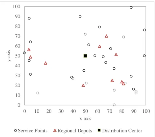
While generating the random problem instances, for each problem size the distribution center is placed at the center of a 100 x 100 grid coordinate system. The locations of the service points in the coordinate system are determined randomly, whereas the locations of the regional depots are determined with the k-means approximation algorithm. With this approach, for each problem size ten different instances in terms of demands and locations of the service points and regional depots are created. In Figure 4.1, instance 1 with 30 service points and 10 regional depots is illustrated on the 100 x 100 grid coordinate system. The distances between the facilities are calculated using Euclidean distance.
25
Figure 4.1 Instance 1 of 30 service points and 10 regional depots
The routing diameter is set as 40 distance units. The daily limit on driving hours is 8 hours and the maximum speed of the vehicles 10 distance units per hour; the maximum length of a route is considered as 80 distance units accordingly. The service time is assumed as 15 minutes, and it is converted into distance units using the maximum speed limit; 15 minutes of service time is represented as 2.5 distance units considering a maximum speed limit of 10 distance units per hour.
The regional depot opening and operating costs are randomly generated between 3000 and 6000. In our study, both the inbound transportation cost to the regional depots from the distribution center and the outbound transportation cost from the regional depots to the service points are represented with staircase cost structures considering three different vehicle sizes. The inbound transportation costs are a function of the vehicle size and the distance between the distribution center and given regional depots. The outbound transportation costs depend only on the selected vehicle type. The values used to represent the inbound and outbound transportation costs are given in Tables 4.1 and 4.2.
0 10 20 30 40 50 60 70 80 90 100 0 10 20 30 40 50 60 70 80 90 100 y-ax is x-axis
26
Table 4.1 Inbound transportation costs used
Volume Break (k) Vehicle Size Vehicle Capacity (Volume)
Cost per Unit Distance
1 Small 1000 100
2 Medium 2000 180
3 Large 5000 250
Table 4.2 Outbound transportation costs used
Volume Break (k) Vehicle Size Vehicle Capacity (Volume) Cost per Vehicle 1 Small 500 2500 2 Medium 1000 4500 3 Large 2000 6500 4.2. Computational Experiments
4.2.1. Summary of Generated Routes
In the input preparation phase of our location-transportation problem, alternative routes are generated by using three different heuristics. The detailed results of the three heuristics for instance 1 with 30 service points and 10 regional depots are given in Appendices A, B and C.
The results of the expanded neighborhood search (ENS) heuristic can be found in Appendix A. For instance 1 with 30 service points and 10 regional depots, 91 alternative routes are generated. The first route (R1) is generated starting from the first regional depot to the service points 1, 2, 4 and 5 in this order. The total distance from the first regional depot to the last service point selected (5) is 60.80 distance units. The total demand covered on this route is 888 units. R6, R30, R41 and R43 are the routes that visit the minimum number of service points which is two. R7, R89 and R91 are the routes that visit the maximum number of service points which is seven. The minimum, average and maximum distances of the routes are 33.64, 53.95 and 88.57 distance units, respectively.
For all the 10 instances of the smallest problem size consıstıng of 30 service points and 10 regional depots, ENS has generated a total of 796 routes. The number of routes formed vary
27
from one instance to another. The instance with minimum number of routes generated for 30 service points and 10 regional depots is instance 2 and incorporates 52 routes. Whereas the instance with maximum number of routes generated for 30 service points and 10 regional depots is instance 10 and has 116 routes. Table 4.3 provides a brief summary of the total number of routes, number of regional depots per service point’s minimum, average and maximum, and number of routes per service point’s minimum, average and maximum. For the sake of completeness, in Table 4.4 and 4.5 similar route summaries for nearest neighbor (NN) and savings algorithm (SAV) are given.
Table 4.3 Summary of ENS generated routes
Problem Size
Total # Routes
# of RD per SP # of Route per SP Min. Avg. Max. Min. Avg. Max.
30 SP & 10 RD 796 6.00 8.85 10.00 2.50 3.06 3.75
50 SP & 15 RD 1684 10.00 11.75 12.50 3.12 3.76 4.17
100 SP & 30 RD 7664 16.67 19.67 20.00 4.35 4.55 5.00
250 SP & 75 RD 47569 17.86 20.05 20.83 5.21 5.73 6.10
Table 4.4 Summary of NN generated routes
Problem Size
Total # Routes
# of RD per SP # of Route per SP Min. Avg. Max. Min. Avg. Max.
30 SP & 10 RD 345 6.00 7.85 10.00 2.73 3.05 3.33
50 SP & 15 RD 645 10.00 11.50 12.50 3.33 3.85 4.55
100 SP & 30 RD 2002 16.67 19.33 20.00 4.35 4.79 5.56
250 SP & 75 RD 8720 19.23 20.67 20.83 5.56 5.98 6.58
Table 4.5 Summary of savings algorithm generated routes
Problem Size
Total # Routes
# of RD per SP # of Route per SP Min. Avg. Max. Min. Avg. Max.
30 SP & 10 RD 713 6.00 8.35 10.00 1.43 1.64 1.88
50 SP & 15 RD 1514 10.00 11.50 12.50 1.61 1.77 2.00
100 SP & 30 RD 6034 16.67 19.33 20.00 1.79 1.86 2.00
28
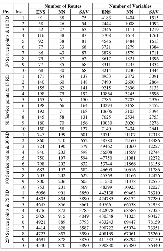
The given routes affect the size of our mathematical problem. For the sake of brevity, the number of routes, corresponding number of variables and binary variables for all the 40 instances using the ENS, NN and savings algorithm are given in Tables 4.6 and 4.7. The nearest neighbor algorithm yields the smallest route set for all the 40 instances. The number of routes generated by the savings algorithm are pretty close to that of the expanded neighborhood search. However, when the routes of instance 1 provided in Appendices A and C are compared, we see that the routes generated by the savings algorithm are significantly shorter due to visiting one or two service points (except R28 where three service points are visited).
29
Table 4.6 Number of routes and number of variables of the three heuristics
Pr.
Ins.
Number of Routes Number of Variables
ENS NN SAV ENS NN SAV
30 S ervic e point s & 1 0 R D 1 91 38 75 4183 1404 1515 2 58 26 54 2444 1008 1092 3 52 27 63 2346 1111 1219 4 116 38 87 5708 1614 1761 5 92 38 81 4546 1484 1613 6 77 33 68 3721 1279 1384 7 86 43 87 3878 1579 1711 8 79 37 62 3617 1321 1396 9 77 35 68 3311 1235 1334 10 68 30 68 3214 1230 1344 50 S ervic e point s & 1 5 R D 1 171 64 137 8933 2872 3091 2 140 60 148 7490 2600 2864 3 155 62 141 9215 2896 3133 4 198 75 192 10864 3245 3596 5 155 61 150 7785 2703 2970 6 198 66 164 10294 3158 3452 7 192 71 168 10606 3103 3394 8 145 58 131 7625 2534 2753 9 180 70 156 10030 3020 3278 10 150 58 127 7140 2434 2641 100 S ervic e point s & 3 0 R D 1 747 199 601 50711 11107 12313 2 860 210 652 58780 12160 13486 3 724 190 579 49462 11060 12227 4 846 203 598 56508 11559 12744 5 750 197 594 47750 11081 12272 6 798 202 632 53744 11866 13156 7 683 192 582 46609 10616 11786 8 703 202 622 45369 11166 12426 9 800 206 605 51530 11378 12575 10 753 201 569 48399 10923 12027 250 S ervic e point s & 7 5 R D 1 5056 901 3850 442138 69463 78310 2 4805 854 3890 424785 68172 77280 3 4647 856 3661 407661 66538 74953 4 4746 872 3785 422078 68586 77325 5 5026 915 4049 430348 71025 80427 6 4921 889 3793 433243 69447 78159 7 4414 828 3587 390722 65074 73351 8 4723 857 3590 408169 67061 75260 9 4691 878 3830 411533 68294 77150 10 4540 870 3890 390830 67380 76440
30
Table 4.7 Number of binary variables and number of constraints of the three heuristics
Pr.
Ins.
Number of Binary Variables Number of Constraints
ENS NN SAV ENS NN SAV
30 S ervic e point s & 1 0 R D 1 313 154 265 542 436 510 2 214 118 202 476 412 468 3 196 121 229 464 414 486 4 388 154 301 592 436 534 5 316 154 283 544 436 522 6 271 139 244 514 426 496 7 298 169 301 532 446 534 8 277 151 226 518 434 484 9 271 145 244 514 430 496 10 244 130 244 496 420 496 50 S ervic e point s & 1 5 R D 1 573 252 471 937 723 869 2 480 240 504 875 715 891 3 525 246 483 905 719 877 4 654 285 636 991 745 979 5 525 243 510 905 717 895 6 654 258 552 991 727 923 7 636 273 564 979 737 931 8 495 234 453 885 711 857 9 600 270 528 955 735 907 10 510 234 441 895 711 849 100 S ervic e point s & 3 0 R D 1 2361 717 1923 2684 1588 2392 2 2700 750 2076 2910 1610 2494 3 2292 690 1857 2638 1570 2348 4 2658 729 1914 2882 1596 2386 5 2370 711 1902 2690 1584 2378 6 2514 726 2016 2786 1594 2454 7 2169 696 1866 2556 1574 2354 8 2229 726 1986 2596 1594 2434 9 2520 738 1935 2790 1602 2400 10 2379 723 1827 2696 1592 2328 250 S ervic e point s & 7 5 R D 1 15468 3003 11850 13087 4777 10675 2 14715 2862 11970 12585 4683 10755 3 14241 2868 11283 12269 4687 10297 4 14538 2916 11655 12467 4719 10545 5 15378 3045 12447 13027 4805 11073 6 15063 2967 11679 12817 4753 10561 7 13542 2784 11061 11803 4631 10149 8 14469 2871 11070 12421 4689 10155 9 14373 2934 11790 12357 4731 10635 10 13920 2910 11970 12055 4715 10755