Active and Merging Galaxies

(1)

Active and Merging Galaxies

Caroline Scott

Astrophysics Group

Department of Physics

Imperial College London

Thesis submitted for the Degree of Doctor of Philosophy to

Imperial College London

(2)

Abstract

Galaxy close pairs are studied to investigate the effects of gravitational interactions on star formation and black hole accretion processes in merger progenitors. We derive star formation rates from near-ultraviolet luminosities; this is a new method for studying mergers and provides unique insight into recent star formation rates. A range of progenitor masses are considered, as well as the separation between merging galaxies and the environment they inhabit. Star formation enhancements in major versus minor close pairs are also considered. Pairs are extracted from the SDSS by identifying galaxies with small angular separation and small recessional velocity difference. Optical photometry in five filters is available for these galaxies. The pairs sample is cross-matched with near-ultraviolet flux measurements from GALEX and specific star formation rates are derived. We study the fraction of active galaxies as a function of separation in close pairs and seek observational evidence for merger activity triggering black hole accretion. Optical emission lines are used to identify progenitors harbouring active galactic nuclei, and the ratio of active galaxies in close pairs is compared to that of non-mergers.

The variable properties of a sample of quasi-stellar objects (QSOs) are analysed. We present optimal QSO classification algorithms that exploit time series variabil-ity features calculated from Pan-STARRS light curves. This groundbreaking work crosses boundaries between astrophysics, statistics and machine learning. Spectro-scopically confirmed QSOs and stars are used to train Support Vector Machine and Random Forest algorithms. We compare and evaluate the outcome of these models then apply them to Pan-STARRS light curves over nine medium deep fields, each covering 7◦-squared and located uniformly across the sky, to predict likely QSO can-didates. We present a host of new variability features to characterise and provide measures of QSO variability.

(3)

List of Tables

2.1 GALEX Baseline Mission Surveys (up to GR4, completed in Fall 2007). . 57

4.1 Median SSFR (yr−1) derived from NUV luminosity for each stellar mass and separation bin. . . 107 4.2 Median SSFR (yr−1) derived from NUV luminosity for each environment

and separation bin. . . 109 4.3 Summary of the SSFR enhancements from the lowest separation bin to

the highest separation bin (i.e. close pairs versus the control sample) from the various analyses in this chapter. . . 123

6.1 Cross Validation results for Stars (S) and QSOs (Q) for RF Models I, II and III. There were 1,468 QSOs and 3,643 stars in the training set. . . 162 6.2 Cross Validation results for Stars (S) and QSOs (Q) for SVM Models I, II

and III. There were 1,468 QSOs and 3,643 stars in the training set. . . 164 6.3 Analysis of Top Features: RF Cross Validation results for combinations of

the top features in g-band only. . . 174 6.4 Predictions from RF Model I, RF Model II and RF Model III. . . 175 6.5 RF blind test evaluation table: precision and recall rates are shown for

Stars and QSOs predicted from RF Models I, II and III. . . 178 6.6 Predictions from SVM Model I, SVM Model II, and SVM Model III. . . . 186 6.7 SVM blind test evaluation table: precision and recall rates are shown for

Stars and QSOs predicted from SVM Models I, II and III.. . . 188

(8)

List of Figures

1.1 Centaurus A . . . 27 1.2 The Hubble tuning fork illustrates Edwin Hubble’s system of

morphologi-cal classification; showing elliptimorphologi-cal, SO, spiral and barred spiral galaxies. . 30 1.3 Top left: M87 elliptical galaxy. Top right: Lenticular galaxy NGC 5866.

Bottom left: M101 spiral galaxy, also known as thePinwheel galaxy. Bot-tom right: NGC 6822, also known asBarnard’s Galaxy. . . 31 1.4 Very Large Array (4.9GHz) image of the radio emission from the quasar

3C 175 atz= 0.77 (Bridle et al., 1994). . . 35 1.5 Illustration of the AGN Unification model.. . . 36 1.6 Top (excerpted from Fan (2012)): Evolution of the density of luminous

quasars. Bottom (excerpted from Bouwens et al. (2011) and Fan (2012)): Rest-frame continuum UV luminosity density atz∼10, and star formation rate density derived from the extinction-corrected luminosity density. . . . 41 1.7 Excerpted from Larson & Tinsley (1978): The two-colour plots for

mor-phologically normal and peculiar galaxies with latitudes|b|>20◦.. . . 45 1.8 Excerpted from Bridge et al. (2007): Number of mergers per galaxy (LIR≥

5×1010 ) as a function of redshift. . . 51 2.1 Excerpt from Morrissey et al. (2007), Table 1. . . 56 2.2 BOSS spectroscopy for two QSO TDSS targets. Left: z = 3.53, right:

z= 5.01 (excerpted from a TDSS presentation by Paul Green, 2013). . . . 59 2.3 Excerpted from Schawinski et al. (2007a): Volume-limited UV

color-magnitude relation.. . . 64 2.4 Excerpted from Yi (2008), originally used by Yi, Demarque & Oemler

(1998): The composite spectrum of the giant elliptical galaxy NGC 4552 shows a classic example of the UV upturn. . . 65 2.5 Excerpted from Shimasaku et al. (2001): Correlation of concentration

in-dex with visually classified Hubble type,T, for 426 galaxies with R50≥200. 67

(9)

2.6 Excerpted from Baldry et al. (2004): Colour-magnitude distributions. (a): Observed bimodal distribution, corrected for incompleteness. (b): Decon-volved and parametrised distributions. . . 70 2.7 Excerpted from Kauffmann et al. (2003a): BPT plot with emission-line

flux ratio [OIII]/Hβ versus the ratio [NII]/Hα for 55,757 galaxies where all four lines are detected with S/N>3. . . 75 3.1 Top: NUV-r colour-magnitude plot. Bottom left: Optical

colour-magnitude plot for galaxies from the optical close pairs sample after our K-correction and extinction correction. Bottom right: NUV-r distribution. 84 3.2 Comparison between our mass estimates with MPA masses for both close

and wide pairs samples. . . 85 3.3 Top: NUV-r against stellar mass plot (left) for the wide pairs (black) and

close pairs (red) samples. Bottom: Stellar mass distribution for the wide pairs (black histogram) and close pairs (red histogram) samples. . . 86 3.4 Halo mass distribution for the close and wide pairs samples.. . . 88 3.5 BPT plots: log10([NII]/Hα) is plotted against log10([OIII]/Hβ) for the

close pairs (top) and wide pairs (bottom). Objects are classified as Star-forming, Transition, LINER or Seyfert depending on the region they in-habit on the BPT diagram. . . 89 3.6 Emission-line luminosity-derived SFRs from the MPA SDSS DR7

cata-logue (black) are compared with NUV photometry-derived SFRs for our wide pairs sample (green) and close pairs sample (red). . . 92 3.7 NUV-r and log10 SFR plot before (top) and after (bottom) internal

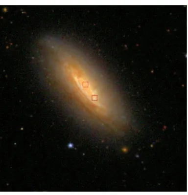
ex-tinction correction. . . 93 3.8 SDSS galaxy: ra, dec = (179.714, 42.7187), z = 0.0019. The red squares

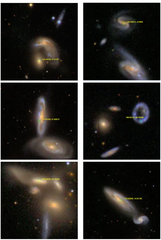
show peaks identified by the pair-extraction code; since there are two peaks our procedure incorrectly concludes that there are two neighbouring galaxies. 95 3.9 Examples from the SDSS online image viewer of galaxy mergers from our

close pairs sample. . . 96 3.10 Examples from the SDSS online image viewer of galaxy mergers from our

close pairs sample. . . 97 3.11 Examples from the SDSS online image viewer of galaxy mergers from our

close pairs sample. . . 98

(10)

3.12 Optical colour-magnitude contour plots showing SDSS galaxies from the close pair catalogue separated by visually classified morphological type. We overplot the visually classified bulge-dominated spirals with green con-tours in the right plot. . . 99 3.13 Redshift distribution (top) and optical colour-magnitude plot (bottom) for

major and minor close pairs samples. . . 101 3.14 Top (left and right): NUV−r distribution for major and minor mergers.

Bottom left: Stellar mass distribution for major and minor mergers. Bot-tom right: Halo mass distribution for major and minor mergers. . . 102 3.15 Emission-line luminosity-derived SFRs from the MPA SDSS DR7

cata-logue are compared with NUV photometry-derived SFRs for our wide pairs sample for the majors sample (left) and minors sample (right). . . 102

4.1 Top: Median NUV-r colours for close and wide pairs binned by separation for both low stellar mass galaxies and high stellar mass galaxies. Bottom: SSFR difference between the separation bin in question and the widest separation bin, for both low and high mass galaxies. . . 106 4.2 Top: Median NUV-r colours for close and wide pairs binned by separation

for pairs in field, group and cluster environments. Bottom: SSFR differ-ence between the separation bin in question and the widest separation bin, for each environment. . . 108 4.3 Median NUV-r and ∆SSFR values for each environment/separation bin

are plotted for low stellar mass galaxies and high stellar mass galaxies. . . 109 4.4 Median NUV-r and ∆SSFR values are plotted for the major mergers

sam-ple (with pair mass ratio>1/3) -top, and and minor mergers sample (with pair mass ratio<1/3) -bottom. . . 111 4.5 Median NUV-r and ∆SSFR values are plotted for the minor mergers

sam-ple split into primary progenitors and secondary progenitors. . . 112 4.6 Median NUV-r colour for minor merger primaries (red) and secondaries

(blue) binned by mass ratio (only close pairs are considered here). . . 114 4.7 Median NUV-rcolour for minor merger primaries (dotted) and secondaries

(dashed) binned by mass ratio. . . 115 4.8 Median NUV-r and ∆SSFR values are plotted for the major mergers

sam-ple (with pair mass ratio>1/3) -top, and and minor mergers sample (with pair mass ratio<1/3) -bottom, for pairs in field (black), group (blue) and cluster (red) environments. . . 116

(11)

4.9 Top: primaries and secondaries for minor mergers in field environments. Bottom: primaries and secondaries for minor mergers in group/cluster environments. . . 117 4.10 Fraction of Transition, LINER and Seyfert galaxies in four separation bins.

Top Left: All masses and environments. Top Right: Restricted to high mass galaxies. Bottom left: High mass galaxies in field environments. Bottom right: High mass galaxies in group environments. . . 119 4.11 Fraction of Transition, LINER and Seyfert galaxies in four separation bins.

Major merger sample (top) and minor merger sample (bottom). . . 120 4.12 Fraction of Transition, LINER and Seyfert galaxies in four separation bins

for major mergers in field and group/cluster environments. . . 121

5.1 Left: Support vectors are the data points located nearest to the hyper-plane. Right: Non-linearly separable data points can often be mapped to a higher dimensional space where they can be separated by a linear hyperplane. . . 130 5.2 Decision tree to classify whether one should or should not play outdoor

sports depending on the weather. In this example the weather conditions are the feature instances. . . 132 5.3 Light curve showing magnitude as a function of modified Julian date

(MJD) for the object with ra = 35.18956671 and dec =−4.85610289 in all five optical bands (g,r,i,z,y). . . 135 5.4 r-band light curves and the corresponding slotted autocorrelation plotted

against time lag (in days) for spectroscopically confirmed QSOs. . . 140 5.5 r-band light curves and the corresponding slotted autocorrelation plotted

against time lag (in days) for spectroscopically confirmed QSOs. The top object is a narrow absorption line QSO. . . 141 5.6 r-band light curves and the corresponding slotted autocorrelation plotted

against time lag (in days) for spectroscopically confirmed narrow absorp-tion line QSOs. . . 142 5.7 r-band light curves and the corresponding slotted autocorrelation plotted

against time lag (in days) for spectroscopically confirmed A-type stars. . . 143 5.8 r-band light curves and the corresponding slotted autocorrelation plotted

against time lag (in days) for spectroscopically confirmed B-type stars. . . 144 5.9 r-band light curves and the corresponding slotted autocorrelation plotted

against time lag (in days) for spectroscopically confirmed F-type stars. . . 145

(12)

5.10 r-band light curves and the corresponding slotted autocorrelation plotted against time lag (in days) for spectroscopically confirmed G-type stars. . . 146 5.11 r-band light curves and the corresponding slotted autocorrelation plotted

against time lag (in days) for spectroscopically confirmed K-type stars. . . 147 5.12 r-band light curves and the corresponding slotted autocorrelation plotted

against time lag (in days) for spectroscopically confirmed M-type stars. . . 148 5.13 Invariance of modifiedg-band features between MD01 and MD09 for Eta

(top), Cusum (middle) and Stetson K (bottom). . . 155 5.14 Invariance of modifiedg-band features between MD01 and MD09 for

Stet-son K (SAC) (top), Eta(SAC) (middle) and P

SAC > e−1 (bottom). . . . 156 6.1 Colour-magnitude and colour-colour plots for the full sample with known

stars and QSOs over-plotted. . . 161 6.2 Bar plot of the absolute value of SVM kernel model weights for g-band

features. The highest SVM kernel weight is indicative of the success of the feature during the classification modelling. . . 166 6.3 Normalised counts of variousg-band feature distributions for Stars (blue)

and QSOs (red) in the training set. The top six features and bottom two features from the SVM kernel weight bar plot are shown. . . 168 6.4 Normalised count of theg-band Skewness distribution for Stars (blue) and

QSOs (red) in the training set with higher resolution binning. . . 169 6.5 Variousr-band features are plotted for Stars and QSOs in the training set. 170 6.6 More two dimensional feature plots. Various r-band features are plotted

for Stars (blue) and QSOs (red) in the training set. . . 171 6.7 More two dimensional feature plots. Various r-band features are plotted

for Stars (blue) and QSOs (red) in the training set. . . 172 6.8 Normalised histogram of RF Model I outputted confidences for QSOs (left)

and stars (right) for predicted objects from the known (spectroscopic) sample (bold) and predicted objects from the unknown sample (dotted). . 176 6.9 Histogram and table showing RF Model I outputted confidences for QSO

predictions from the full unknown sample. . . 176 6.10 Blind test results. Normalised histogram of RF Model I outputted

confi-dence for the QSOs (left) and stars (right) for spectroscopically confirmed and falsely predicted objects.. . . 179 6.11 QSO predictions summary for each RF model. . . 180

(13)

6.12 The top two plots showg-band magnitude and colour-magnitude plots for QSOs predicted by RF Model III but not RF Models I or II. Bottom: Normalised histogram of confidences for QSO predictions. . . 181 6.13 RFu−g and g−r colour-colour plots. . . 182 6.14 RFg-band magnitude andu−g colour-magnitude plots. . . 183 6.15 These plots show QSOs predicted by RF Model I but not RF Model III. . 184 6.16 Normalised histogram of SVM Model I outputted confidences for QSOs

(left) and stars (right) for predicted objects from the known and unknown samples. . . 187 6.17 Histogram and table showing SVM Model I outputted confidences for QSO

predictions from the full unknown sample. . . 187 6.18 Blind test results. Normalised histogram of SVM Model I outputted

confi-dence for the QSOs (left) and stars (right) for spectroscopically confirmed objects and falsely predicted objects.. . . 189 6.19 QSO predictions summary for each SVM model. . . 190 6.20 The top two plots showg-band magnitude and colour-magnitude plots for

QSOs predicted by SVM Model III but not SVM Models I or II. Bottom: Normalised histogram of confidences for QSO predictions. . . 191 6.21 SVM u−g and g−r colour-colour plots. . . 192 6.22 SVM g-band magnitude andu−g colour-magnitude plots. . . 193 6.23 These plots show QSOs predicted by SVM Model I but not SVM Model III.195 6.24 RF Model I confidences (top) and SVM Model I (bottom) for various RF

and SVM Confidence Q cutoffs. . . 196 6.25 Colour-colour (top) and colour-magnitude (bottom) plots for predicted

QSOs with RF Model I and SVM Model I Q confidences ≥0.7 in green and Q confidences≥0.9 in red. . . 197

(14)

Publications and Conference

Appearances

• “Star Formation and AGN Activity in Interacting Galaxies: A Near-UV Perspective”,

Caroline Scott & Sugata Kaviraj, 2014, MNRAS, 437, 2137

• “Star Formation and AGN Activity in Major and Minor Mergers”, Caroline Scott, 2014, MNRAS, submitted

• “QSO Selection Model Using Light Curve Variability Features from Pan-STARRS”,

Caroline Scott, Pavlos Protopapas, Paul Green, Dae-Won Kim, Eric Morgan-son, 2014, MNRAS, in progress

• “Mauna Kea Observatories, Hawaii”,

Article written by Caroline Scott for Icy Science Magazine, February 2014,

http://www.icyscience.com/Magazine.html

• “Identifying Quasars from their Variability Features”,

Caroline Scott, Post-Graduate Research Physics Symposium, Imperial College London, U.K., 2013, presentation

• “Star Formation and AGN Activity in Interacting Galaxies: A Near-UV Perspective”,

Caroline Scott, Interacting Galaxies and Binary Quasars Meeting, Interna-tional Centre for Theoretical Physics, Trieste, Italy, 2012, presentation

• “Star Formation and AGN Activity in Massive Interacting Galax-ies”,

Caroline Scott, International Astronomical Union General Assembly XXVIII, Beijing, China, 2012, presentation

(15)

• “IAU Meeting, China”,

Article written by Caroline Scott for Astronomy Wise Magazine, October 2012,

http://www.scribd.com/doc/108494427/Astronomy-Wise-October-EZine

• “Let’s Talk... Caroline Scott Interview”,

Interview by Astronomy Wise Magazine, July 2012,http://astronomy-wise. blogspot.com/2012/07/astronomy-wise-e-zine-is-out-now-july.html

• “Studying Close Pairs in the Near-UV”,

Caroline Scott & Sugata Kaviraj, National Astronomy Meeting, Manchester, UK, 2012,poster

Declaration and Copyright

This thesis is my own work, except where explicitly indicated in the text.

The copyright of this thesis rests with the author and is made available under a Cre-ative Commons Attribution Non-Commercial No DerivCre-atives licence. Researchers are free to copy, distribute or transmit the thesis on the condition that they at-tribute it, that they do not use it for commercial purposes and that they do not alter, transform or build upon it. For any reuse or redistribution, researchers must make clear to others the licence terms of this work.

Caroline Scott 19 February 2015

(16)

- To all family, friends and colleagues who have been a continuous source of support and inspiration during the process of writing this thesis

-“Willst du ins Unendliche schreiten, Geh nur im Endlichen nach allen Seiten.”

(Do you want to stride into the infinite? Then explore the finite in all directions.) - Johann Wolfgang von Goethe

Sunset from Mauna Kea Observatories, Hawaii, during an observing trip at the James Clerk Maxwell Telescope in January 2014.

(17)

Foreword

The last century has born witness to some of the greatest revelations about our physical surroundings in history. Technological innovations have allowed scientists to probe microscopic to macroscopic scales in greater detail than ever before. Discov-eries in particle physics are leading to a more detailed understanding of the building blocks of our natural world. Currently, advancing research into the Higgs-particle endeavours to uncover the nature of mass and the force of gravity. Astronomical explorations are allowing us to translate these fundamental laws to describe physical conditions and processes in other planets, stars and galaxies. Even the nature of the Universe itself can be explored using data from a number of modern telescopes that have been specifically designed for cosmological studies. Such studies seek to explain the formation of large-scale structures that now harbour galaxies, to un-cover the ratio of ordinary to unknown/exotic matter, and to probe the nature of the mysterious force known as dark energy that drives the accelerated expansion of the Universe.

When two or more galaxies merge we are granted a rare glimpse into the act of evolution within the Universe. The strength of gravitational forces present during a merger can induce changes in the morphology, star formation rate, central black hole mass and internal galactic processes of progenitors. In the early Universe, the galaxy population would have been very different to how it appears now, almost 14 billion years later. We endeavour to observe galaxies at different stages in this merging act and to understand the role that mergers play in galaxy evolution. We also aim to study the internal mechanisms of active galaxies, to understand their role in galaxy evolution and to determine whether interactions with other galaxies may trigger the process of black hole accretion in active galaxies. The aim of this thesis is to contribute to these areas of research by providing new insight and analyses of active and merging galaxies. To facilitate this, we use data from a range of new-generation astronomical instruments.

The research presented in this thesis was conducted between Imperial College London (my home institution), the Harvard-Smithsonian Center for Astrophysics

(18)

(where I was granted a Smithsonian Astrophysical Observatory Predoctoral Fel-lowship between April 2012 and April 2014) and Harvard’s Institute for Applied Computational Science (where I was granted a Research Fellowship between De-cember 2012 and April 2014). At Imperial College, I was supervised by Sugata Kaviraj and Stephen Warren; we worked within the field of galaxy mergers (this work is detailed in Chapters 3 and 4). At Harvard I was supervised by Pavlos Pro-topapas and Paul Green; we applied contemporary computer science methods to classify active galaxies (this work is detailed in Chapters 5 and 6).

This thesis begins by introducing the reader to underlying topics and essen-tial terminology in the field of galaxy evolution. We then introduce the tools and techniques used to obtain and prepare data for our research in Chapter 2. Original research is presented in Chapters 3 to 6. To conclude, we summarise and discuss this work in Chapter 7.

(19)

19

Chapter 1 Introduction

Overview

In this introductory chapter we present a review of the standard paradigm of struc-ture formation in the framework of the ΛCDM cosmological model. We discuss the prominent features of this model and give examples of its successes and failures when tested with observational data. We describe the two main competing models that have dominated the field of galaxy evolution in recent decades; monolithic collapse and hierarchical formation through galaxy mergers. Both models are evaluated and we explain why the hierarchical formation model is more convincing within a ΛCDM framework and in better agreement with observations. As new studies are presented using increasingly reliable observational data and powerful computer simulations, many refinements have been made to the hierarchical model of galaxy evolution. We summarise and evaluate the results of many relevant studies here. A precise parametrisation of the merger rate with redshift can provide meaningful constraints for modelling hierarchical evolution; various observational studies that have esti-mated the merger rate are reviewed.

We familiarise the reader with nomenclature in this field of research by introduc-ing terms such as dark matter and dark energy. Various galaxy types are described that were initially categorised morphologically by Edwin Hubble; these include ellip-tical, spiral, lenticular and irregular galaxies. Active galaxies and potential mech-anisms of black hole accretion in active galaxies are introduced. Observations of photometric variability in active galaxies are discussed, and theoretical propositions that this variability could arise from accretion disk instabilities are evaluated.

(20)

1.1 The Standard Paradigm for Structure Formation 20

1.1 The Standard Paradigm for Structure

Forma-tion

Constituents of the Universe

The standard paradigm states that the Universe was initially radiation dominated; i.e. the radiation density was higher than the matter density and Cosmological con-stant density. However, expansion over time led to cooling and the radiation density decreased rapidly (∝ a−4; where a(t) is the scale factor1) and the Universe shifted into its current matter-dominated era2. This matter is present in two fundamental forms; baryonic and non-baryonic. The word baryon is derived from the Greek word ‘heavy’, and baryonic matter typically describes heavy particles; protons, neutrons, and all atoms and ordinary matter constructed from these particles.

The term ‘dark matter’ was initially used by Fritz Zwicky (1933) when he ap-plied the Virial Theorem to the Coma galaxy cluster and found that the expected total galaxy mass was much higher than that implied by their observed luminos-ity. Jan Oort (1932) had already observed that stellar motions within the Milky Way implied that the galactic plane mass should be higher than that inferred from observed matter. Nearly fifty years later, dark matter was proposed to explain rota-tion curve measurements of stars within spiral galaxies that were inconsistent with standard Newtonian dynamics; observable matter alone is not sufficient to explain the surprisingly high velocity of distant objects in orbit when confined to standard Newtonian gravity (Rubin, Ford & Thonnard, 1980). The true nature of dark matter is currently unknown, but it is hypothesised to consist of mostly exotic and yet-to-be-discovered non-baryonic matter that does not absorb or emit detectable amounts of electromagnetic radiation. Baryonic matter could potentially constitute some of the dark matter fraction in the form of massive compact halo objects that emit undetectable levels of electromagnetic radiation; gravitational microlensing surveys have been utilised to search for evidence of this form of matter (Paczynski, 1986; Griest, 1991; Ricotti & Gould, 2009; Iocco et al., 2011).

1_{The scale factor describes expansion in a homogeneous and isotropic Universe. The expansion}

rate, orHubble parameter, ˙a/a is an expression frequently encountered in Cosmology.

2_{This shift to a matter dominated Universe occurred as the matter density decreases less rapidly}

than the radiation density (ρradiation∝a−4 whereasρmatter ∝a−3); physically this reflects a loss

in photon energy due to redshifting, leading to particles becoming non-relativistic and constituting ordinary matter.

(21)

Λ

CDM

The ΛCDM model is currently the most widely-accepted cosmological model stem-ming from the Big Bang theory (e.g. Liddle, 2003; Rebolo et al., 2004; Navarro et al., 2010; Komatsu et al., 2011; Dunkley et al., 2011; Hinshaw et al., 2013; Planck Col-laboration, 2013). It balances simplicity with impressive accuracy at matching many observed properties of the cosmos such as accelerated expansion and the large-scale structure distribution. This model describes a homogeneous and isotropic Universe which features a cold dark matter component and a cosmological constant term, Λ (as predicted from Einstein’s equations of general relativity). The cosmological constant has negative pressure and is believed to describe the accelerating expan-sion whereby galaxies are generally found to be moving away from each other and the Universe appears to be expanding in all directions. Cosmological expansion was predicted theoretically by Georges Lemaˆıtre in 1927 as a consequence of gen-eral relativity, and was shortly after observed by Edwin Hubble by measuring the recessional velocities of nearby objects (Lemaˆıtre, 1927; Hubble, 1929). The hy-pothetical force driving accelerated expansion has been termed ‘dark energy’, and although the nature of this force is not yet understood, dark energy is routinely included in most cosmological models. It is currently postulated that the Universe comprises ∼4.9% baryonic matter, ∼26.8% dark matter and ∼68.3% dark energy (Planck Collaboration et al., 2013b).

Evaluating

Λ

CDM

Over the last decade, observational data from instruments such as the Wilkinson Mi-crowave Anisotropy Probe (WMAP) and Planck have helped to corroborate various aspects of the ΛCDM model through studies of anisotropies in the cosmic microwave background (CMB; see explanation below). Detailed supernovae measurements in-dicate an accelerated expansion in the Universe consistent with ΛCDM (Paal, Hor-vath & Lukacs, 1992; Riess et al., 1998; Knop et al., 2003; Wang & Tegmark, 2005; Astier et al., 2006; Blake et al., 2011). However, many gaps exist within this stan-dard model. There are a number of observations for which ΛCDM does not offer explanations by itself, and extensions are frequently proposed to explain observed properties that ΛCDM does not predict directly.

For example, the very early Universe is thought to have undergone a period of momentous inflation which led to the flat, homogeneous and isotropic properties that we observe. Inflation offers an explanation for an issue that stems from ΛCDM known as the ‘horizon problem’, where isolated regions of the Universe that have no

(22)

apparent causal connection seem to have evolved as if causally connected with re-gards to consistent temperature and curvature. Inflation is thought to have carried quantum fluctuations to outside of the Hubble radius (R =c/H, for Hubble param-eter, H, and speed of light,c), leading to isotropy. Various models of inflation have been proposed, and this is currently an active area of research in cosmology. Also additional to ΛCDM, baryogenesis models seek to explain how the matter fraction came to outweigh that of the anti-matter fraction in the early Universe (since the Big Bang is predicted to have produced equal matter/anti-matter fractions), allowing pockets of matter to form and the observed structure of the cosmos to emerge.

The main contender to ΛCDM is Modified Newtonian Dynamics (MOND), proposed by Mordehai Milgrom (Milgrom, 1983). This seeks to explain the puzzle of rotation curve measurements by modifying aspects of Newtonian gravity at small accelerations, such that objects at large radius in gravitational orbits have a larger velocity. The dark matter versus MOND debate is ongoing and is an active area of research for cosmologists and particle physicists (Bertone, Hooper & Silk, 2005; Kroupa et al., 2010; Famaey & McGaugh, 2012; Milgrom, 2013); MOND is beyond the scope of this thesis and we assume a ΛCDM cosmological model throughout.

Analysing the Seeds of Structure Formation

Analysis of the CMB is particularly useful for studying the evolution of large-scale structure in the Universe, as the relics of structure over-densities and under-densities are encoded in light that has been travelling since the era of decoupling. Prior to this time, the Universe was hot, dense and opaque due to the absorption of elec-tromagnetic radiation by hydrogen plasma. Recombination describes the transition period where cooling due to expansion allowed radiation and plasma to cool enough for neutral hydrogen and helium to form, and thus for structure to emerge. This is estimated to have occurred ∼400,000 years after the big bang. Recombination led to the decoupling of photons that were no longer scattered by electrons in the hot dense plasma of protons and electrons, and the light from this decoupling period is still reaching us from all directions. This light has now been redshifted from the microwave to the radio band.

The CMB power spectrum has been mapped in detail by COBE (Fixsen et al., 1996; Jaffe et al., 2001), WMAP (Spergel et al., 2003; Bonaldi et al., 2007) and most recently Planck (Planck Collaboration et al., 2013a). It is observed to have a black body spectrum with incredible precision. However, tiny fluctuations quan-tified in the power spectrum reveal slight under-densities and over-densities at the

(23)

time of decoupling. ΛCDM predicts that primordial density fluctuations should be isotropic and Gaussian distributed, and therefore much about the validity of this model can be learned from studying CMB anisotropies (Eriksen et al., 2004; Emir Gümrük¸cüoglu, Contaldi & Peloso, 2007; Planck Collaboration et al., 2013c). With the latest Planck data, anisotropies in the CMB are measured with incredible precision. These observations must be satisfied by all credible cosmological mod-els, enabling tight constraints to be placed on inflationary and structure formation models.

Primordial density fluctuations are predicted to have been amplified during inflation shortly after the Big Bang and to have undergone continuous contrac-tion/expansion thereafter into regions of dark matter over-densities/under-densities. The primordial density fluctuations can be traced by minute temperature fluctua-tions, and are estimated to have varied by an order of 10−5 _{at recombination. These}

density perturbations are thought to have continually evolved under their own grav-itational instability, causing regions with deep potential wells to be inhabited by concentrated baryonic matter; this evolution could then have led to structure for-mation. By ‘structure’, we mean condensed matter on all scales from galaxies to galaxy clusters and superclusters (also known as ‘galaxy filaments’; these are the largest structures presently known) as well as the extended void regions between.

‘Jeans instability’ occurs when the force of gravitational collapse is stronger than the outward pressure from gas or radiation. Since dark matter does not inter-act with radiation, the outward radiation pressure does not oppose dark matter from flowing freely into gravitationally dense regions, leading to gravitational clustering and forming a cosmic web of dark matter halos. Once this network of structure was established galaxies would then have formed hierarchically by the merging of dark matter halos (White & Rees, 1978; White & Frenk, 1991; Kauffmann, White & Guiderdoni, 1993; Parkinson, Cole & Helly, 2008). It is important to understand the structure of dark matter clustering, as this determines the spatial distribution of galaxies and therefore affects how galaxies interact and evolve. The distribution of galaxies has been mapped by surveys including the 2dF Galaxy Redshift Survey (Magliocchetti & Porciani, 2003; Cole et al., 2005; Ribeiro et al., 2009). The Mil-lennium Simulation (Boylan-Kolchin et al., 2009) was a three-dimensional N-body simulation using more than 1010 _{particles to trace dark matter structure evolution}

to its present state. It provided a mostly convincing re-enactment of structure for-mation (e.g. Fakhouri, Ma & Boylan-Kolchin, 2010). However, it predicted more small-scale dark matter sub-halos than there is observational evidence for; we might expect to see objects such as dwarf galaxies and globular clusters inhabiting these

(24)

regions.

Protogalactic clouds of concentrated baryonic matter in the central regions of dark matter halos would then form and cool to below the virial temperature, finally collapsing under their own gravity to form the very first stars (Silk, 1977; Abel, Bryan & Norman, 2002; Bromm et al., 2009), which are known as ‘population III’ stars. Through a series of mergers, the first galaxies could then begin to grow and evolve morphologically. Some galaxies have been observed using Hubble Ultra Deep Field Imaging dating back to only 600 million years after the Big Bang (e.g. Bouwens et al., 2010), allowing us to place constraints on the era when the first galaxies formed. It will be shown in Section 1.2 that many morphological types of galaxies now exist.

1.1.1 Monolithic Collapse

The monolithic collapse model was proposed by Eggen, Lynden-Bell & Sandage (1962). It is contradicted by many recent observations and is generally neglected in favour of the hierarchical formation model (see Section 1.1.2), however, we illustrate it here due to its historical significance. Much work in the past has been devoted to modelling and simulating galaxy formation from a monolithic collapse perspective, and thus it plays a significant role in how research in the field of galaxy evolution has progressed.

The monolithic collapse model suggests that galaxies are formed by the collapse of massive gas clouds under their own gravity in a short and efficient burst. In this model, early-type galaxies formed at high redshift with little structural evolution since. These are often referred to as ‘red-and-dead’ galaxies; all stars are thought to have formed in a single starburst and then evolved passively from then on (Eggen, Lynden-Bell & Sandage, 1962; Larson, 1975). Thomas, Greggio & Bender (1999) suggest that these initial starbursts must last less than 1 Gyr to reproduce the stellar populations observed in elliptical galaxies. Indeed, Kriek et al. (2008) found that∼45% of K-bright massive galaxies already have evolved stellar populations by

z ∼ 2.3 with little ongoing star formation. This model offers a natural explanation for observations of cosmic downsizing (see Section 1.1.3). It is also consistent with the small scatter and lack of evolution with redshift observed in the fundamental plane for early-type galaxies (see Section 1.2.1).

It was shown by Kauffmann, Charlot & White (1996) using the colours of 125 local galaxies (from the Canada-France Redshift Survey) that only∼1/3 of local el-liptical and SO galaxies could have been assembled and contained passively evolving

(25)

stellar populations byz = 1. Kauffmann et al. concluded that other processes must play a role in their evolution, such as morphological disturbances and recent star formation caused by mergers. Van Dokkum et al. (2008) observed that the quies-cent early type galaxies in the sample used by Kriek et al. (2008) are very compact (with median effective radius re= 0.9 kpc) compared to galaxies of similar mass in

the nearby Universe (which have sizes ∼5 kpc) and that fully assembled early-type galaxies only comprise at most ∼10 % of K-selected quiescent galaxies at z ∼ 2.3. This shows that considerable evolution must have taken place afterz ∼2.3 (through dry mergers or other processes) and provides strong evidence against the monolithic collapse model.

Monolithic collapse also fails to satisfy other observational properties; the rota-tion of the protogalactic cloud would imply that stars would move in elliptical orbits in the same direction (a trend which is not observed), and we would expect globular clusters to have formed at the same time within a narrow time frame (however, we observe a broad range in globular cluster ages). If monolithic collapse were to be considered as a viable model, elements of hierarchical evolution would still have to be considered to account for these observational discrepancies.

1.1.2 Hierarchical Evolution of Galaxies through Mergers

The hierarchical model of galaxy formation attributes the evolution of galaxies to the process of repeated mergers between smaller galaxies (e.g. Toomre & Toomre, 1972; Fall & Efstathiou, 1980; Kauffmann, White & Guiderdoni, 1993; Cole et al., 2000; Steinmetz & Navarro, 2002; Jiang et al., 2008; Brook et al., 2012; Shankar et al., 2013; Wetzel et al., 2013). Because of this sequential evolution from smaller to larger galaxies, the standard paradigm for galaxy evolution is known as a ‘bottom-up’ model.

Most galaxies with substantial spheroidal components are thought to harbour supermassive black holes at their centre; these are expected to be linked with prop-erties of the host galaxy (Kormendy & Richstone, 1995; Magorrian et al., 1998; Di Matteo, Springel & Hernquist, 2005; Ishibashi & Fabian, 2014). When a merger takes place it is thought that the surrounding dark matter halos merge and the gas cools and condenses, forming a rotating disk at the halo’s centre in which star for-mation begins to take place (Somerville & Primack, 1999; Kauffmann & Haehnelt, 2000; Hatton et al., 2003).

As the galaxies merge some of this gas is funnelled into the black hole nuclei of the progenitor galaxies and the rest is thought to be used up in starbursts. A

(26)

tight correlation can be seen between supermassive black hole mass and velocity dispersion in the galactic bulge, adding confidence to the idea that there is a strong link between spheroid formation and black hole growth (Richstone et al., 1998; Cattaneo, Haehnelt & Rees, 1999; Kauffmann & Haehnelt, 2000; Monaco, Salucci & Danese, 2000; Cavaliere & Vittorini, 2000; Gebhardt et al., 2000; Haehnelt & Kauffmann, 2000; Hu, 2008). During the final stages of a merger, the supermassive black holes orbit and finally merge (Begelman, Blandford & Rees, 1980; Debuhr, Quataert & Ma, 2011). The small percentage of the remaining gas is accreted onto the new black hole (this is thought to occur over a timescale of order 107 years) with the rest of the gas being transformed into stars (e.g. Kauffmann & Haehnelt, 2000). General relativity predicts that gravitational waves are emitted during the coalescence of super massive black holes, and so final stage mergers provide a potential observational test for general relativity.

Disk galaxies are thought to be formed through the acquisition of angular mo-mentum via tidal torques in interacting dark matter halos (Silk, 2003; Dekel, Sari & Ceverino, 2009; Agertz, Teyssier & Moore, 2011). Gravitational contraction leads to rotational support as angular momentum is conserved, and baryonic cooling within dense regions of the resulting disk leads to star formation. These low mass, spiral-shaped galaxies are then predicted to undergo a succession of mergers that result in higher mass galaxies, eventually forming massive elliptical-shaped galaxies (Toomre, 1978; Schweizer, 1982; Wright et al., 1990; Bournaud, Jog & Combes, 2007). After conducting three-dimensional simulations between gravitationally interacting bodies (each containing ∼104 _{particles), Barnes (1988) found that the observed}

morpho-logical parameters and intrinsic properties of galaxies could be reproduced by this model of merging disk galaxies. In this work, Barnes modified merger simulations originally conducted by Toomre & Toomre (1972) to include dark matter halos in the merger scenario. Even without the inclusion of dark matter halos, and with much more basic simulations (between only two bodies), Toomre and Toomre came to the same conclusion: galaxy mergers explain many of the properties that we see in neighbouring galaxies, such as tidal tails and bridges.

Kauffmann & Charlot (1998) present a model of elliptical galaxy formation in which the majority of stars are thought to have formed in disk galaxies that then go through a series of mergers to form ellipticals. In this work they assume that supernovae explosions allow the transfer of metals between the stars, the cold gas and the hot gas halo components (i.e. it is a non-closed box model). The semi-analytic models they adopted imply that the inter-cluster medium between elliptical galaxies in cluster environments will have seen very little evolution sincez <1. This

(27)

is because more than 80% of metals belonging to galaxies with circular velocities

< 250km s−1 _{will have been ejected through supernova explosions for} _{z >} _{1. In}

this model, bright elliptical galaxies are thought to have formed from the merging of massive disk galaxies, whereas faint ellipticals form from lower mass mergers. Since mergers inherit most of the independent stellar populations of the progenitor galaxies as well as new stars that are formed throughout the merger, modelling the resulting stellar population of a merger is a difficult task.

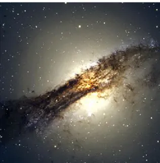
Figure 1.1: Centaurus A (http://en.wikipedia.org/wiki/File:Centaurus A.jpg).

A local example of a galaxy merger is Centaurus A (see Figure 1.1); the fifth brightest galaxy observed from Earth. Although the subject of debate, this appears to be an elliptical galaxy in the process of accreting a spiral galaxy (Tubbs, 1980). Active star formation and black hole accretion are seen in Centaurus A. Our own galaxy, the Milky Way, and the spiral galaxy Andromeda (which is located approxi-mately 2.5 million light years from Earth) are currently approaching each other and are expected to merge within 5 billion years (Cox & Loeb, 2008).

Modelling Hierarchical Growth

Despite impressive advances in computing, N-body simulations are still unable to fully reproduce the dynamical evolution of galaxies since many physical processes are not fully understood. Accurate star formation and dust models are required, as well as models describing the accretion of gas and dust onto central black holes. Semi-analytic processes adopting Monte Carlo simulations can be used to simulate

(28)

hierarchical structure growth (see Section 1.3.4) by assuming cosmological density perturbation theory and using parameters such as radiative cooling, star formation, supernova feedback, the stellar initial mass function, metallicity, dust extinction, stellar winds, and merging rates of galaxies (Baugh et al., 1998; Somerville & Pri-mack, 1999; Kauffmann & Haehnelt, 2000; Hatton et al., 2003; Dubois et al., 2012, etc.). When using Monte Carlo methods, processes must be simplified; spherical symmetry and certain flow properties must be assumed (e.g. Cole et al., 2000). As well as permitting cosmological modelling for large numbers of galaxies, semi-analytic simulations are very useful for testing feasible models within galaxies; such as modelling the evolution between an active galactic nucleus, black hole growth, bulge formation and star formation (see Section 1.3.3).

N-body simulations offer an alternative to Monte Carlo simulations; however, such methods are computationally heavy, resolution limited, and extremely time consuming (e.g. Heggie & Hut, 2003). Steinmetz & Navarro (2002) used N-body methods to simulate the formation and evolution of a galaxy population and con-cluded that hierarchical growth is likely to play a significant role in galaxy evolution.

1.1.3 Downsizing: An Issue with the Hierarchical

Forma-tion Model?

Using a nearly complete sample of 393 Keck spectroscopically observed galaxies, Cowie et al. (1996) found that the most massive and luminous galaxies appear to have already formed and ceased star formation at high redshift; whereas low mass galaxies have prolonged star formation that is still ongoing. They called this trend ‘downsizing’. Bower, Lucey & Ellis (1992) found that≤10% of the stellar population in early-type and SO galaxies was formed in starbursts in the last 5 Gyr. Ellis et al. (1997) built upon the work of Bower et al. and showed that the bulk of the stellar population in dominant spheroidal galaxies in clusters would have formed before

z ' 3. Terlevich, L´opez & Terlevich (2007) used a sample of local HII galaxies, which typically have low mass and intense star formation, to investigate downsizing within low mass galaxies. They found that the lowest mass systems are generally younger with lower metallicity than the more massive ones and hence downsizing can even be seen within low mass distributions of galaxies.

This presents an apparent contradiction to hierarchical formation since this model predicts that the formation of massive galaxies should have taken placeafter

that of lower mass galaxies, thus we might expect to see more recent star formation in massive galaxies. However, Neistein, van den Bosch & Dekel (2006) commented

(29)

1.2 The Hubble Sequence and Hubble Types 29

that the downsizing effect is not necessarily contradictory to a hierarchical model of halo clustering if cooling and baryonic feedback effects are included in merger models. Their simulations show that with certain parameterisations of these pro-cesses, efficient star formation can be extended in low mass galaxies, but quenched in high mass galaxies. Faber et al. (2007) show that downsizing is likely to be the result of various processes that quench star formation in blue galaxies, causing them to migrate into the red sequence; this would offer an explanation for the observed increase in red sequence galaxies since z ∼ 1. Examples of quenching processes in-clude the massive halo quenching model (Dekel & Birnboim, 2006; Cattaneo et al., 2006), satellite quenching (Faber et al., 2007) and active galactic nuclei feedback (see Section 1.3.3).

Stringer et al. (2009) used the Millennium Simulation as a basis for mock obser-vations of halo clustering, then used semi-analytic methods to simulate the evolution of a population of galaxies. Utilising theradio-modefeedback available ingalform

(see Section 1.3), they were able to reproduce the effects of cosmic downsizing within a hierarchical scenario. However, their model led to the over-excessive quenching of star formation for intermediate mass galaxies, and failed to reproduce the observed colour distribution of galaxies for their full redshift range (0.4< z <1.4).

Observations of cosmic downsizing show that star formation in massive galaxies at early times must have been more efficient than it is now. To be fully accepted, hierarchical formation models must be further developed in order to provide an explanation for these effects.

1.2 The Hubble Sequence and Hubble Types

In The Realm of the Nebulae, (1936), Edwin Hubble proposed a morphological clas-sification scheme; this is illustrated in the well-known Hubble tuning fork in Figure 1.2. The Hubble classification sequence uses the morphological properties of galaxies to classify them as either elliptical, spiral, lenticular or irregular. We now look at the properties of each Hubble type.

1.2.1 Elliptical

Defined by their ellipsoidal shape (see Figure 1.3, top left), these galaxies have approximately elliptical isophotes3_{. Elliptical galaxies have the property 0}_.₃_._≤_1,

3_{Isophotes are lines of constant surface brightness. It has been estimated that only one third}

(30)

Figure 1.2: The Hubble tuning fork illustrates Edwin Hubble’s system of mor-phological classification; showing elliptical, SO, spiral and barred spiral galaxies.

where = _ab and b_a is the ratio of semi-minor to semi-major axes. Elliptical galaxies are assigned a Hubble type according to 10×(1−), thus the Hubble type for elliptical galaxies ranges from E0 (with circular isophotes) to E7 (with axis ratio 0.3). An axis ratio _.0.3 has never been observed; this is believed to be due to theFirehose instability. The Firehose instability arises because for _. 0.3 (an approximate axis ratio 1:3) the system is susceptible to bending in the direction perpendicular to the elongated axis which results in the elongated axis ratio becoming shorter; i.e. the galaxy becomes rounder (Hernquist, Heyl & Spergel, 1993; Jessop, Duncan & Levison, 1997)4_{. Elliptical galaxies generally have a de Vaucouleurs brightness}

profile given as follows;

IE(r) = Iee−7.67((r/re)

1/4₋₁₎

. (1.1)

Elliptical galaxies are the most massive galaxy types and have a high escape velocity. Gas is needed to fuel star formation and elliptical galaxies have a smaller gas content than other galaxy types. Using interferometric 12CO(1-0) observations, Davis et al. (2013) finds that, although elliptical galaxies show less molecular gas than spiral galaxies, the gas content is dependent on the environment of the ellipti-cal, with ellipticals in higher density environments showing less gas and implying a different path of evolution from field ellipticals. When supernovae explode, remain-ing interstellar gas can be heated and ejected from the galaxy by resultremain-ing galactic winds (Mathews & Baker, 1971; Larson, 1974; Loewenstein, 2013). This effect is

isophotes (Combes et al., 1990; Nieto, 1988).

4_{The Firehose instability is also thought to aid the formation of bulges in barred spiral galaxies}

(31)

Figure 1.3: Top left: M87 elliptical galaxy. Situated near the centre of the Virgo cluster, M87 boasts a high number of globular clusters (∼10,000); Canada-France-Hawaii Telescope, J.C. Cuillandre, Coleum. Top right: Lenticular galaxy NGC 5866; imaged by HST and released in the original NASA press release. Globular clusters inhabit the outer halo, each containing nearly ∼ 1,000,000 stars. Bottom left: M101 spiral galaxy, also known as the Pinwheel galaxy; composite image from 51 HST exposures and ground based images and released by NASA. It is situated in the Ursa Major constellation (25MLyrs from Earth) and spans nearly twice the diameter of the Milky Way. Bottom right: NGC 6822, also known asBarnard’s Galaxy is an irregular galaxy member of our Local Group in the constellation of Sagittarius. It is a small galaxy and has low surface brightness yet it contains relatively bright HII regions which have sparked a lot of interest in studying it.

http://apod.nasa.gov/apod/ap040616.html

http://www.spacetelescope.org/images/opo0624a/

http://hubblesite.org/newscenter/archive/releases/2006/10/image/a http://www.astronomy-mall.com/Adventures.In.Deep.Space/barnard.htm

(32)

dampened somewhat by radiative cooling but still has dramatic effects for lowering gas and metallicity levels, especially in less massive galaxies where the gravitational potential well is shallower.

Observations in optical wavebands indicate that little star formation takes place in ellipticals (Baum, 1959; Sandage & Visvanathan, 1978; Bower, Lucey & Ellis, 1992). The ‘Fundamental Plane’ is a three-dimensional space with axes of velocity dispersion, effective radius and effective surface brightness. Elliptical galaxies only span (approximately) a two-dimensional subspace of the Fundamental Plane (Djor-govski & Davis, 1987) and show little scatter (Jorgensen, Franx & Kjaergaard, 1996; Cappellari et al., 2006; Graham, 2013); a lack of evolution with redshift is shown in this scatter (Bower, Lucey & Ellis, 1992), implying that the bulk of star formation took place by z = 2 (Peebles, 2002). This lack of observable recent star formation led to massive elliptical galaxies being described as ‘early-type’ or ‘red and dead’. However, more sensitive indicators of star formation show that a significant number of ellipticals do in fact show ongoing star formation (e.g. Kaviraj et al., 2007; Ford & Bregman, 2013). Kaviraj et al. (2007) used NUV-r colours from ∼2100 early-type galaxies from SDSS DR3 (crossmatched with GALEX measurements for NUV magnitudes) and found that at least 30% show evidence of recent star formation to a 95% confidence level.

For quite some time, observational evidence has implied that early-types have a cold gas content which could be used to fuel star formation. Cold gas (≤100K) has been identified in early-types using HI 21cm emission line measurements (Knapp, Turner & Cunniffe, 1985; Wardle & Knapp, 1986; Morganti et al., 2006; Serra et al., 2012) and CO emission line measurements (Wiklind & Rydbeck, 1986; Phillips et al., 1987; Knapp & Rupen, 1996; Young, 2005; Young et al., 2011). Since dust radiates in the far-IR, the IRAS satellite has granted a new perspective by which to measure interstellar dust and to map dust regions that could potentially fuel star formation. Knapp et al. (1989) used an IRAS sample of∼1150 early type galaxies and found a significant interstellar dust content in a large fraction of early type galaxies. Row-lands et al. (2012) compare the dust properties using submillimetre measurements of elliptical and spiral galaxies and find that submillimetre-selected ellipticals can show as much dust as typical spirals.

1.2.2 Spiral

Hubble classified spiral galaxies as either standard spirals (S) or barred spirals (SB); he acknowledged that these classifications are not disjoint and a small proportion

(33)

of galaxies lie between between S and SB. Spiral galaxies are rotating disk galaxies characterised by a central bulge and spiral arms extending from the centre, or from the edge of the bar in the case of an SB galaxy (see Figure 1.3, bottom left).

The central bulge is generally a concentrated region of older stars (Graham, 2013). The spiral arms are thought to be caused by spiral gravitational density waves which are independent of the rotational motion of the stars and gas within the galaxy; they are visible as a result of orbiting matter being compressed in these regions when passing through (Lin & Shu, 1964; Kim & Kim, 2014). The increased density in spiral arms causes gas clouds to approach their Jeans limit; if this limit is surpassed the gas clouds will collapse to create starbursts. As a result spiral arms are often inhabited by young, OB-type stars which makes them brighter and bluer. Spirals tend to have younger stellar populations than elliptical galaxies. When plotted on optical colour-magnitude diagrams spirals are usually found in the so-called blue cloud, with the bluer colours indicating that more star formation is taking place, whereas ellipticals tend to inhabit the red region (Strateva et al., 2001; Bell et al., 2003). This bimodal colour distribution provides a simple, yet not always reliable, way to distinguish between spiral and elliptical galaxies. Hubble’s classifi-cation system was modified by de Vaucouleurs (1959) with particular emphasis on categorising spiral galaxies to include more detailed features such as diffuse/broken spiral arms with a lack of bulge component (Sd, SBd), and highly irregular appear-ance with a lack of bulge component (Sm, SBm). In Hubble’s classification system these galaxies were grouped together as Irr galaxies. The light profile of the bulge in spirals is generally described by a de Vaucouleurs profile, with that of the disk following an exponential brightness profile given by

IS(r) =Ise−(r/rs). (1.2)

1.2.3 Lenticular/SO

SO galaxies lie between the morphological classifications of elliptical and spiral galax-ies and are also known as lenticular galaxies because of their lentil-like shape (see Figure 1.3, top right). They are disk galaxies with bulges and usually with unclear spiral arms, yet they generally have low star formation rates like elliptical galaxies because they have been stripped of most of their interstellar gas (Cappellari et al., 2006). Hubble later modified the SO classification to distinguish between non-barred lenticular, SO, galaxies and barred, SBO, lenticular galaxies. Hubble died before publishing some modifications to his classification system, however Allan Sandage, the successor to Hubble at the Mt. Wilson and Palomar Observatories, collected

(34)

1.3 The Role of Active Galaxies in Evolutionary Models 34

Hubble’s notes and continued his work (de Vaucouleurs, 1959).

1.2.4 Irregular

Galaxies which did not fit into any of the three above morphological classifications were categorised by Hubble as irregular (Hunter & Elmegreen, 2006). These galax-ies, which lack rotational symmetry and a dominating nucleus, account for∼2-3% of the population and are usually star forming; often at a rate similar to that of spiral galaxies (Hunter, 1997). They are morphologically peculiar galaxies, for example the Magellanic Clouds (irregular dwarf galaxies), Messier 82 (although this was first classified as irregular from optical observations, spiral arms have since been detected in the near-Infrared) and NGC 6822 (see Figure 1.3, bottom right).

1.3 The Role of Active Galaxies in Evolutionary

Models

1.3.1 Active Galactic Nuclei

Active galactic nuclei (AGN) activity occurs in the central region of massive active galaxies, outputting radiation that traverses most of the electromagnetic spectrum (Lynden-Bell, 1969). This substantial emission is thought to be triggered by the accretion of gas and dust onto a central supermassive black hole. An accretion disk forms from the in-falling interstellar material and generates a range of extreme physical processes surrounding the galaxy nucleus (Rees, 1984; Lin & Papaloizou, 1996; Ulrich, Maraschi & Urry, 1997; Mirabel & Rodr´ıguez, 1999; Kembhavi & Narlikar, 1999; S¸adowski et al., 2013; Suzuki & Inutsuka, 2014). During the accretion process, gravitational potential energy from in-falling material is converted into kinetic energy which can very efficiently be transformed into heat and radiated away due to friction within the accretion disk. The origin of AGN activity is not yet understood, but it could potentially be triggered by tidal interactions or mergers with other galaxies; this is a question that we address in Chapter 4.

Photometric and variability properties are distinguished from non-active galax-ies, where the majority of emitted light comes from stellar or nebular activity. Quasars stellar radio sources) and their radio-quiet companions QSOs (quasi-stellar objects) are the most luminous types of AGN. They have broad emission lines and an extremely high luminosity emanating from the compact galactic nucleus, al-lowing them to be detected at high redshift as point-sources (Villata et al., 2006;

(35)

Mortlock et al., 2011). The accretion disk is generally surrounded by a dusty torus and optically thick plasma that can obscure our view of the active nucleus. In some radio-loud quasars, two radio lobes can be seen extending roughly symmetrically from quasars (de Vries, Becker & White, 2006); these are often connected by out-flowing jets of relativistic particles that are thought to provide a path for energy transfer between the compact central core and radio lobes (see Figure 1.4). To-gether, these radio components have been observed to span up to ∼1 Mpc. Optical jets were first observed extending from the active elliptical galaxy M87 (located in the Virgo cluster) by Curtis (1918) (Mirabel & Rodr´ıguez, 1999).

Figure 1.4: Very Large Array (4.9GHz) image of the radio emission from the quasar 3C 175 atz = 0.77 (Bridle et al., 1994). The radio emission spans nearly 200 kpc. Notice that the radio jets extend from a compact source, the galaxy center, located at (∆α,∆δ)=(0,0).

The lower redshift, lower luminosity analogs of Quasars and QSOs are the Seyfert Type I galaxies. Still characterised as active nuclei with high luminosity and broad emission lines, Seyferts tend to have host galaxies resolvable by optical telescopes. Type II QSOs and Seyfert Type II galaxies are similar but show only narrow emission lines. Other types of AGN have been identified; such as BL Lacs (named because the galaxy BL Lacertae is a prototypical example), radio galaxies (radio-bright elliptical galaxies), and blazars (compact quasars where the relativis-tic jets are directed at the observer). Orientation-based unification schemes have attempted to group different types of AGN into one standard model where we at-tribute various properties (such as luminosity, emission-width etc.) to the angle

(36)

(37)

active galaxies. Time series variability is observed over a wide range of wavelengths and time-scales from hours to years (Heckman, 1976; Hook et al., 1994; Hawkins, 2002; MacLeod et al., 2012, references therein), with more luminous objects showing less variability (Vanden Berk et al., 2004) and at longer timescales (Hawkins, 1993; Giveon et al., 1999). More than 90% of quasar light curves in Stripe 82 show vari-ability at the 0.03 mag level on timescales of a few years (Sesar et al., 2007). There are many potential sources of variability, mainly due to accretion disk instabilities or processes taking place in jet regions (Rees, 1984; Kawaguchi et al., 1998; Tr`evese, Kron & Bunone, 2001; Pereyra et al., 2006). Other potential sources include super-novae bursts (e.g. Terlevich et al., 1992) and microlensing events by compact objects such as stars situated along the line of sight (e.g. Hawkins, 1993). Continuum vari-ability can be observed from gamma to radio wavelengths, with most studies so far having been conducted in the optical band.

Different types of AGN tend to show different variability properties. Quasars tend to vary more at shorter wavelengths (de Vries, Becker & White, 2003). Since emission from blazars is dominated by the jets, they usually show strong (i.e. >1 mag) flux variations on a range of time-scales, from days to months, and over a broad range of frequencies, from radio to gamma. BL Lac and OVV galaxies often show large-amplitude, short-timescale (i.e. days) variability that could be caused by relativistic beaming effects (e.g. Bregman et al., 1990; Fan & Lin, 2000; Vagnetti, Trevese & Nesci, 2003). In UV-optical bands, Seyfert I and quasars generally show less variability (<0.5 mag), on larger time-scales of more than a few months; al-though large variations (>1 mag) on time-scales of days have been detected using X-rays in some Seyfert galaxies.

A structure function analysis measures the power distribution over a range of timescales to describe the temporal structure of variations (Simonetti, Cordes & Heeschen, 1985; Hughes, Aller & Aller, 1992; de Vries, Becker & White, 2003; Vanden Berk et al., 2004; de Vries et al., 2005). The structure function is defined as

S(τ) = ( 1 N(τ) X i<j [m(i)−m(j)]2 )1/2 (1.3)

for time intervals τ = tj −ti, for all exposures i < j. For a total of N exposures, de Vries et al. (2005) group all n(n−1)/2 possible time-lag permutations into bins containing at least 200 measurements. The structure function outputted for each bin is the root mean square of the magnitude variations. Hughes, Aller & Aller (1992) found that the total structure functions of QSOs and BL Lacs show similar