A Maximum Entropy Method for Solving the Boundary Value Problem of Second Order Ordinary Differential Equations

(1)

The Aquila Digital Community

Faculty Publications

10-3-2018

A Maximum Entropy Method for Solving the Boundary Value

Problem of Second Order Ordinary Differential Equations

Congming Jin

Zhejian Sci-Tech University

Jiu Ding

University of Southern Mississippi, [email protected]

Follow this and additional works at: https://aquila.usm.edu/fac_pubs

Part of the Mathematics Commons

Recommended Citation

Jin, C., Ding, J. (2018). A Maximum Entropy Method for Solving the Boundary Value Problem of Second Order Ordinary Differential Equations. Journal for Mathematical Physics, 59(10).

Available at: https://aquila.usm.edu/fac_pubs/15561

This Article is brought to you for free and open access by The Aquila Digital Community. It has been accepted for inclusion in Faculty Publications by an authorized administrator of The Aquila Digital Community. For more information, please contact [email protected].

(2)

JOURNAL OF MATHEMATICAL PHYSICS59, 103505 (2018)

A maximum entropy method for solving the boundary

value problem of second order ordinary

differential equations

Congming Jin1,a)_{and Jiu Ding}2

1_{Department of Mathematics, Zhejiang Sci-Tech University, Hangzhou 310018, China} 2_{Department of Mathematics, University of Southern Mississippi, Hattiesburg,} Mississippi 39406-5045, USA

(Received 16 March 2018; accepted 5 September 2018; published online 3 October 2018)

We propose a new method to solve the boundary value problem for a class of sec-ond order linear ordinary differential equations, which has a non-negative solution. The method applies the maximum entropy principle to approximating the solution numerically. The theoretical analysis and numerical examples show that our method is convergent.Published by AIP Publishing.https://doi.org/10.1063/1.5029856

I. INTRODUCTION

The maximum entropy principle was proposed by Jaynes in 1957,1which has been widely used in statistical physics, image processing, networks, etc.2–6The maximum entropy method has been applied to computing absolutely continuous invariant measures of discrete dynamical systems7–9 and non-negative solutions of Fredholm integral equations.10,11Theory and numerical experiments have shown that the maximum entropy method is efficient when splines are used as moment functions.12

There are a lot of numerical methods for solving differential equations, such as finite element methods, finite difference methods, finite volume methods, spectral methods, etc. These methods are not universal. There may be effective special techniques for special differential equations, for example, the adaptive method and the multiscale method. Numerically solving two-point boundary value problems for second order ordinary differential equations is often quite simple to formu-late, but sometimes still needs particular techniques to get better results. For example, in Refs.13

and14, an initial value technique for singularly perturbed two-point boundary value problems using an exponentially fitted finite difference scheme was proposed. In Refs.15and16, a method based on B-splines for solving a self-adjoint singularly perturbed two-point boundary value problem was given. In Ref.17, a method was provided for the numerical solution of second order linear ordinary differential equations in the high-frequency regime. In Ref.18, an exponentially fitted finite difference scheme was proposed for singularly perturbed two-point boundary value problems for second order ordinary differential equations with two small parameters multiplying the derivatives. In Ref.19, a new method based on a single layer Legendre neural network model was developed to solve initial and boundary value problems.

The maximum entropy method was used to solve linear differential equations20_{and the} Fokker-Planck equation.21 _{This method gave approximate solutions evaluated at some given points. The} employed moment functions there are trigonometric functions. Another type of moment functions were used to solve some time dependent partial differential equations.22,23_{In Ref.}₂₄_{, higher order} moments with respect to{x,x2_,_x3_,_{. . .}_,_xN_}_{were evaluated to solve the Fokker-Planck equation. Such} moment functions are all globally defined on the whole domain with single algebraic expressions, like all the classic maximum entropy methods, and consequently the instability issue is present due to the fact of ill-conditioning for the classic approach. Moreover, the maximum entropy principle behind

a)_{Author to whom correspondence should be addressed:}_{[email protected]}

(3)

all such methods was applied to a discrete system of algebraic equations, instead of the continuous system directly out of the Boltzmann entropy, for the Lagrange multipliers, so another error occurs in addition to the one from the use of finitely many moments. In our new method, we not only employ piecewise cubic functions to eliminate the ill-conditioning but also apply the maximum entropy principle to the whole involved integrals without choosing the evaluation points in the domain of integration.

When the solution of the boundary value problem is guaranteed to be non-negative, the maximum entropy principle, which is mainly used for the numerical recovery of unknown density functions, can be effectively explored, at least in theory. Here we try this kind of exploration by using the maximum entropy method to numerically solve the two-point boundary value problem for sec-ond order ordinary differential equations that have non-negative solutions. We shall employ cubic splines to form moment functions used in our method since such functions are locally nonzero and globally twice continuously differentiable. Our scheme provides a new way to think of the numerical solution of the special class of differential equations. In Sec.II, the maximum entropy method is proposed for the solution of the boundary value problem of a second order linear dif-ferential equation, and its convergence will be established in Sec.III. We provide an approximate maximum entropy method for nonlinear boundary value problems in Sec. IV. In Sec.V, some numerical experiments are given to show the efficiency of the method. The conclusion is given in Sec.VI.

II. A MAXIMUM ENTROPY METHOD FOR BOUNDARY VALUE PROBLEMS OF SECOND ORDER ORDINARY DIFFERENTIAL EQUATIONS

We consider the two-point boundary value problem for a second order linear ordinary differential equation      Ly(x)≡ −d dx p(x)dy_dx(x)+q(x)y(x)=f(x), a<x<b, y(a)=β1,y(b)=β2, (1) where the given function p is differentiable andq and f are continuous functions. Suppose the two-point boundary value problem has a non-negative solution, and our purpose is to calculate it numerically.

For some boundary value problem, the maximum principle25 can guarantee that it has a non-negative solution, as the following theorem shows.

Theorem 2.1. If p(x)≥0, f(x)≥0, and q(x)>0for x∈(a, b) and β1≥0and β2≥0, then the solution y∗of the boundary value problem(1)satisfies that y∗(x)≥0for all x∈[a, b].

Proof. Let ˆxbe the minimum point ofy∗in (a,b) andy∗(ˆx)<0. Theny∗0(ˆx)=0 andy∗00(ˆx)≥0, and so f(ˆx)=−_dxd pdy∗ dx (ˆx) +q(ˆx)y∗(ˆx)=−p(ˆx)d 2_y ∗ dx2(ˆx) +q(ˆx)y∗(ˆx)<0,

which contradicts to the fact thatf(ˆx)≥0. ◽

For the purpose of using a piecewise polynomial maximum entropy method to numerically recover the non-negative solution y∗ from above, we first divide the interval [a, b] into n equal subintervals of length h = (b a)/n. The nodes of the partition are xi = a + ih, i = 1, 0, 1, . . .,n,n + 1, where x1 andxn+1 are the two artificial ones to help dealing with the boundary

condition.

We shall use the cubic B-spline functions associated with the above partition of [a,b] to develop our maximum entropy method. They are constructed via translation and scaling from the “mother” cubic B-spline function defined on (∞,∞),26which can be directly calculated out as follows by the

(4)

103505-3 C. Jin and J. Ding J. Math. Phys.59_{, 103505 (2018)}

fundamental property of its being second order continuously differentiable:

B(x)=                          1 6(x 3_{+ 6}_x2_{+ 12}_x_{+ 8),} ₋₂_≤_x_{≤ −}_1, 1 6(−3x 3₋₆_x2_{+ 4),} ₋₁_≤_x_≤_0, 1 6(3x3−6x2+ 4), 0≤x≤1, 1 6(−x 3_{+ 6}_x2₋₁₂_x_{+ 8),} ₁_≤_x_≤_2, 0, x<[−2, 2].

Then the corresponding cubic B-spline functions are Bi(x)=B _x₋_x i h , i=−1, 0,. . .,n+ 1.

Now we begin to develop the maximum entropy method with the cubic B-spline functions. Since y∗solves Eq. (1), there is the equality

−d dx p dy∗ dx ! +qy∗=f.

Fori=1, 0,. . .,n+ 1, multiplyingBito both sides of the above equality and integrating fromato b, we get b a Bi(x) " −d dx p dy∗ dx ! (x) +q(x)y∗(x) # dx= b a Bi(x)f(x)dx. (2) Using integration by parts two times gives

− b a Bi(x)_dxd pdy∗ dx (x)dx =−Bi(x)p(x)dy_dx∗(x) b a+ b a p(x)y∗0(x)B_i0(x)dx =−Bi(x)p(x)dy_dx∗(x) b a+p(x)y∗(x)B_i0(x) b a − b a y∗(x) f p0₍_x₎_B0 i(x) +p(x)B 00 i(x) g dx. For eachi=1, 0,. . .,n+ 1, let

˜ gi(x)=−[p0(x)Bi0(x) +p(x)B 00 i (x)] +q(x)Bi(x) (3) and ˜ mi= b a Bi(x)f(x)dx. Then equality (2) can be written as

b a y∗(x)˜gi(x)dx+ " −Bi(x)p(x) dy∗ dx(x) b a+p(x)y∗(x)B 0 i(x) b a # =m˜i. (4) Now we evaluate the expression in the brackets above for various indices i. Clearly Bi(a) =Bi(b) = 0 andBi0(a) =B

0

i(b) = 0 fori= 2, 3,. . .,n2. So for such indicesi, (4) is reduced to b

a

y∗(x)˜gi(x)dx=m˜i. SinceBi(b) =B_i0(b) = 0 fori=1, 0, 1 and

B−1(a)= 1 6, B0(a)= 2 3, B1(a)= 1 6, B0₋₁(a)=−1 2h, B 0 0(a)=0, B 0 1(a)= 1 2h,

(5)

the equalities in (4) withi=1, 0, 1 become              ∫_aby∗(x)˜g−1(x)dx+ 1₆p(a)dy_dx∗(a) +₂1_hp(a)y∗(a)=m˜−1, ∫_aby∗(x)˜g0(x)dx+ ₃2p(a)dy_dx∗(a) =m˜0, ∫aby∗(x)˜g1(x)dx+ 1₆p(a)dy_dx∗(a)−₂1_hp(a)y∗(a) =m˜1.

In the above equalities, multiplying the first and last by 4 and subtracting the second lead to b a y∗(x)[4˜g−1(x)−g˜0(x)]dx=4 ˜m−1−m˜0− 2 hp(a)y∗(a) and b a y∗(x)[4˜g1(x)−g˜0(x)]dx=4 ˜m1−m˜0+ 2 hp(a)y∗(a). Similarly, fromBi(a) =B0_i(a) = 0 fori=n1,n,n+ 1 and

Bn−1(b)= 1 6, Bn(b)= 2 3, Bn+1(a)= 1 6, B_n0₋₁(b)=−1 2h, B 0 n(b)=0, B 0 n+1(b)= 1 2h, the equalities (4) withi=n1,n,n+ 1 are

             ∫aby∗(x)˜gn−1(x)dx−1₆p(b)dy_dx∗(b)−₂1_hp(b)y∗(b)=mñ−1, ∫_aby∗(x)˜gn(x)dx−₃2p(b)dy_dx∗(b) =mñ, ∫_aby∗(x)˜gn+1(x)dx−1₆p(b)dy_dx∗(b) +₂1_hp(b)y∗(b) =mñ+1,

from which it follows that b a y∗(x)[4˜gn−1(x)−gñ(x)]dx=4 ˜mn−1−mñ+ 2 hp(b)y∗(b) and b a y∗(x)[4˜gn+1(x)−gñ(x)]dx=4 ˜mn+1−mñ− 2 hp(b)y∗(b). Define the following numbers, which are called themoments, as

mi=                  4 ˜m−1−m˜0−2_hp(a)y∗(a), i=0, 4 ˜m₁−m˜₀+2_hp(a)y∗(a), i=1, ˜ mi, i=2,. . .,n−2, 4 ˜mn−1−m˜n+ 2_hp(b)y∗(b), i=n−1, 4 ˜mn+1−m˜n−2_hp(b)y∗(b), i=n and the correspondingmoment functionsas

gi(x)=                        4˜g−1(x)−g˜0(x), i=0, 4˜g1(x)−g˜0(x), i=1, ˜ gi(x), i=2,. . .,n−2, 4˜g_n−1(x)−g˜n(x), i=n−1, 4˜gn+1(x)−g˜n(x), i=n. (5)

Then the following is valid: b

a

y∗(x)gi(x)dx=mi, fori=0, 1,. . .,n.

The above equalities provide a framework for numerically solving the boundary value problem (1) by the maximum entropy method. That is, among all the non-negative solutionsyof the equality constraints

(6)

b a

y(x)gi(x)dx=mi, fori=0, 1,. . .,n, (6) we find the one, denoted asyn, which maximizes the correspondinggeneralized differential entropy defined by H(y)=− b a y(x) lny(x)dx+ b a y(x)dx, ∀y∈L1(a,b),y≥0. (7)

Namely, we solve the following constrained optimization problem:11 max ( H(y) :y≥0, b a y(x)gi(x)dx=mi, i=0, 1,. . .,n ) . (8)

To get the expression of the solution of (8), we need the following lemma. Lemma 2.1. Given any two non-negative functions f, g∈L1_{(a, b),}

b a f(x)dx− b a f(x) lnf(x)dx≤ b a g(x)dx− b a f(x) lng(x)dx.

Proof. In the Gibbs inequality27

u−ulnu≤v−ulnv, ∀u,v≥0,

letting u = f(x) and v = g(x) and then integrating both sides, we obtain the required integral

inequality. ◽

Theorem 2.2. The non-negative function in L1(a, b) that maximizes the entropy functional(7) under the constraints(6)is

yn(x)=exp* , n X i=0 λigi(x)+

-if the constantsλ0,. . .,λn, which are called the Lagrange multipliers, satisfy the given constraints X gi(x)exp*. , n X j=0 λjgj(x)+/ -dx=mi, i=0,. . .,n. (9)

Proof. Lety∈L1(a,b) be non-negative and satisfy the moment constraints b

a

y(x)gj(x)dx=mj,j=0,. . .,n. Then, using Lemma 2.1, we have

H(y)=− b a y(x) lny(x)dx+ b a y(x)dx ≤ b a yn(x)dx− b a y(x) lnyn(x)dx = b a yn(x)dx− n X i=0 λi b a y(x)gi(x)dx = b a yn(x)dx− n X i=0 λimi = b a yn(x)dx− b a yn(x)       n X i=0 λigi(x)       dx = b a yn(x)dx− b a yn(x) lnyn(x)dx=H(yn).

(7)

This shows thatyn is an optimal solution. Furthermore, sinceH is strictly concave,28 the optimal

solution is unique. ◽

The nonlinear equation (9) can be solved by Newton’s method as in other maximum entropy algorithms. Since the support of eachBi(x) is local, from (3) to (5), the Jacobian matrix of the nonlinear equation is banded, which can be shown to be positive definite with the same technique as in Ref.8. For more details of the maximum entropy method, see Refs.7,8, and11.

III. CONVERGENCE OF THE METHOD

The weak convergence of the classic maximum entropy method was first obtained by Mead and Papanicolaou in their pioneering paper,29and Borwein and Lewis28gave the first rigorous conver-gence analysis for the moment problem under theL1-norm, based on a more general convergence theory in the context of topological spaces, as developed in Ref.30. The norm convergence of our cubic spline maximum entropy method for the boundary value problem (1) can be established via the general convergence theory from Ref.28. To put our algorithm in the framework for the con-vergence analysis in Ref.28, we divide [a,b] into 2r equal subintervals in succession withr= 2, 3,. . .. And we useyr instead ofy2r to denote the approximate maximum entropy solution of (1)

with respect to the corresponding partition of [a,b] into 2requal sub-intervals. In other words, we calculate the functionyramong all non-negative functions ofL1(a,b) that satisfy the 2r+ 1 moment constraints (6).

Denote byDr the feasible set of the maximum entropy problem, that is, the collection of all non-negative solutions of (6). ThenDr ⊃Dr+1for allr. Clearlyyrsolves

max    H(y) :y∈Dr= r \ k=2 Dk      .

On the other hand, it is easy to see that the unique solutiony∗of the original boundary value problem (1) is the unique solution of

max    H(y) :y∈ ∞ \ r=2 Dr      .

Using the same idea for the convergence analysis in Ref.11, we can prove the following theorem. Theorem 3.1. Suppose that H(y∗)>∞. Let yr be the maximum entropy solution of (8)with respect to the equal partition of [a, b] into 2rsubintervals. Thenlimr→∞kyry∗k1= 0.

As for the convergence rate of our algorithm, from Theorem 4.7 of Ref.28,

kyr−y∗k1≤dre dr 2 =_O₍_d r), where dr=inf      lny∗− 2r X i=0 αigi ∞ :∀α₀,α1,. . .,α2r     

is the minimal distance of the function lny∗to the subspace spanned by allgi’s. From the expressions (5) of the moment functions gi’s, which involve the differential operator L as well as the cubic B-spline functions Bi’s, we see that in general, it is not an easy task to estimatedr theoretically. However, our numerical experiments in Sec. Vshow that the convergence rate of the method is

ky_n y∗k1 =O(1/n2), whereyn is the approximate solution of the boundary value problem when [a,b] is partitioned intonequal sub-intervals.

IV. A CLASS OF NONLINEAR BOUNDARY VALUE PROBLEMS

The idea of the above maximum entropy method for linear boundary value problems may be extended to solving nonlinear boundary value problems numerically, resulting in an approximate

(8)

maximum entropy method for a class of boundary value problems of nonlinear ordinary differential equations.

Let the right-hand side of the boundary value problem (1) bef(x,y) that is a general nonlinear differentiable function of its variables. Motivated by the explicit expression of maximum entropy solutions, we choose an initial vector (λ0

0,. . .,λ 0

n) for the Lagrange multipliers and form the initial approximate maximum entropy solution

y0_n(x)=exp* , n X i=0 λ0 igi(x)+

-for the boundary value problem. Next, we substitutey0_ninto the right side of the differential equation for the variableyin the expression of f(x,y) so that we have obtained the corresponding linear boundary value problem (1) as

     Ly(x)≡ −_dxd p(x)dy_dx(x)+q(x)y(x)=f(x,y0_n(x)), a<x<b, y(a)=β1,y(b)=β2. (10) We can apply the maximum entropy method developed in Secs.IIandIIIto solve (10). Then we get new valuesλ1₀,. . .,λ1n of the Lagrange multipliers, and a new approximate maximum entropy solution of the nonlinear boundary value problem is

y1_n(x)=exp* , n X i=0 λ1 igi(x)+ -. By the same token, we substitutey1

ninto the right-hand side of (10), solve the updated linear boundary value problem by the maximum entropy method, and get the next approximate maximum entropy solutiony_n2. From this iterative process, we can get a sequence of approximate maximum entropy solutions{y0_n,y1_n,. . .}by our maximum entropy method. The fourth example of Sec.Vwill illustrate this approach for a famous boundary value problem.

V. NUMERICAL RESULTS

In this section, we present some numerical examples for solving boundary value problems for second-order linear ordinary differential equations using our method.

Example 1. The first example is

     y00₋_y₌_x_{, 0}_<_x_<_1, y(0)=0, y(1)=1, whose exact solution is

y(x)=2(e x₋_e−x₎ e−e−1 −x.

TheL1-norm errorskyny∗k1and theL∞-norm oneskyny∗k∞of the numerical approximations are shown in TableI. The numerical solutions converge, and the convergence rate is approximately O(1/n2) for theL1-norm errors andO(1/n) for theL∞-norm errors.

Example 2. We consider a singular perturbation two-point boundary value problem16

     −εy00+y=1 + 2√ε exp −√x ε + exp x_√−1 ε , 0<x<1, y(0)=0, y(1)=0,

and the exact solution is

y(x)=1−(1−x) exp −√x ε ! −xexp x√−1 ε ! .

(9)

TABLE I. Errors for Example 1.

n L1-norm error L∞-norm error 4 5.3×103 2.6×102 8 1.6×103 1.3×102 16 4.5×104 _6.4_×₁₀3 32 1.3×104 _3.2_×₁₀3 64 3.6×105 _1.6_×₁₀3 128 9.9×106 8.0×104 256 2.7×106 4.0×104

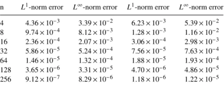
Example 3. The third example is also from Ref.16, which is another singularly perturbed two-point boundary value problem

       −εy00+y=x, 0<x<1, y(0)=1, y(1)=1 + exp −√1 ε , whose exact solution is

y(x)=x+ exp −√x ε

!

.

The numerical results for Examples 2 and 3 are shown in TablesIIandIII, respectively. The second and third columns are the results whenε = 1/16 and the fourth and fifth columns are the results whenε= 1/32. We see that the convergence rate for Example 2 is the same as for Example 1, but bothL1-norm andL∞-norm errors are roughlyO(1/n2) for Example 3.

Example 4. The last example is a nonlinear two-point boundary value problem for the so-called Thomas-Fermi equation,31

TABLE II. Errors for Example 2.

n L1_{-norm error} _L∞_{-norm error} _L1_{-norm error} _L∞_{-norm error}

4 4.99×102 _1.91_×₁₀1 _6.62_×₁₀2 _0.27_×₁₀1 8 1.45×102 _9.21_×₁₀2 _1.89_×₁₀2 _1.26_×₁₀1 16 4.40×103 _4.5_×₁₀2 _5.45_×₁₀3 _6.10_×₁₀2 32 1.31×103 _2.26_×₁₀2 _1.63_×₁₀3 _3.02_×₁₀2 64 3.81×104 _1.13_×₁₀2 _4.80_×₁₀4 _1.51_×₁₀2 128 1.09×104 5.67×103 1.37×104 7.56×103 256 3.05×105 2.84×103 3.89×105 3.79×103

TABLE III. Errors for Example 3.

n L1-norm error L∞-norm error L1-norm error L∞-norm error 4 4.36×103 _3.39_×₁₀2 _6.23_×₁₀3 _5.39_×₁₀2 8 9.74×104 8.12×103 1.28×103 1.16×102 16 2.36×104 2.07×103 3.06×104 2.98×103 32 5.86×105 5.24×104 7.56×105 7.63×104 64 1.46×105 _1.32_×₁₀4 _1.88_×₁₀5 _1.93_×₁₀4 128 3.65×106 _3.31_×₁₀5 _4.70_×₁₀6 _4.86_×₁₀5 256 9.12×107 _8.29_×₁₀6 _1.18_×₁₀6 _1.22_×₁₀5

(10)

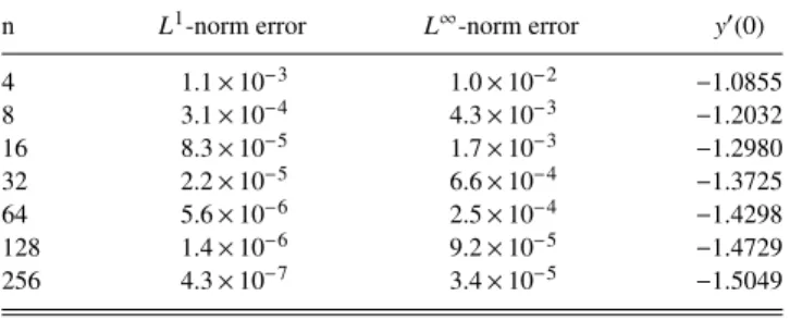
TABLE IV. Errors for Example 4.

n L1-norm error L∞-norm error y0(0) 4 1.1×103 1.0×102 1.0855 8 3.1×104 4.3×103 1.2032 16 8.3×105 _1.7_×₁₀3 _1.2980 32 2.2×105 _6.6_×₁₀4 _1.3725 64 5.6×106 _2.5_×₁₀4 _1.4298 128 1.4×106 9.2×105 1.4729 256 4.3×107 3.4×105 1.5049        y00₌y_√32(x) x , 0<x<+∞, y(0)=1, limx→∞y(x)=0,

whose exact solution is unknown. There are lots of papers about the above equation; see Ref.32

and the references therein. To test our method in Sec.IV, we consider the following boundary value problem of the Thomas-Fermi equation on a finite interval

       y00=y 3 2(x) √ x , 0<x<1, y(0)=1, y(1)=y∗(1),

where the boundary condition is chosen according to an approximate analytic solution in the following:33 y∗(x)= (1 + 1.810 61x12 + 0.601 12x)2 (1 + 1.810 61x12 + 1.395 15x+ 0.771 12x 3 2 + 0.214 65x2+ 0.047 93x 5 2)2 . (11)

In this example, the right-hand side of the differential equation contains the unknown solutiony. So the moments used in the maximum entropy method cannot be defined as in Eq. (5). However, we can follow the iterative process described in Sec.IVto obtain an approximate maximum entropy solution accurate to a desired precision.

TheL1-norm errorskyny∗k1and theL∞-norm oneskyny∗k∞of the numerical approximations are shown in TableIV, wherey∗ is given by (11). The numerical solutions seem to converge, and the convergence rate is approximatelyO(1/n2) for theL1-norm errors and faster thanO(1/n) for the L∞

-norm errors. We also list an estimated value of the derivativey0

(0) by our method, which is important in physics32_{that obtained a better approximate value}_{1.588 071}_{. . .}_for_y0_{(0) after a rather} complicated iterative process.

VI. CONCLUSIONS

In this study, we proposed a maximum entropy method, based on cubic B-spline functions, to approximate non-negative solutions of boundary value problems of second order linear ordinary differential equations. The theoretical analysis and numerical results show the convergence of the method. Furthermore, since the main numerical work is solving a system of nonlinear equations for the Lagrange multipliers without ill-conditioning, the algorithm is stable and easy to be implemented. We also applied this method to the boundary value problem for some special second order nonlinear ordinary differential equations.

The maximum entropy method with splines as moment functions provides a serious and promis-ing numerical approach for the recovery of non-negative function solutions of differential, integral, and operator equations. Extending our method to multi-variable differential equations and other dif-ficult problems in stochastic analysis and random dynamical systems will be our future work when non-negative or density functions need our computational exploration.

(11)

ACKNOWLEDGMENTS

The research of Congming Jin was partially supported by the National Science Foundation of China under Grant No. 11571314 and the “521” Talents Program of Zhejiang Sci-Tech University.

1_{E. Jaynes, “Information theory and statistical mechanics,”}_{Phys. Rev.}₁₀₆_{, 620–630 (1957).}

2_{S. Press´e, K. Ghosh, J. Lee, and K. A. Dill, “Principles of maximum entropy and maximum caliber in statistical physics,”} Rev. Mod. Phys.85(3), 1115–1141 (2013).

3_{M. Tseitlin, A. Dhami, S. S. Eaton}_{et al.}_{, “Comparison of maximum entropy and filtered back-projection methods to}

reconstruct rapid-scan EPR images,”J. Magn. Reson.184(1), 157–168 (2007).

4_{S. Horvt, E. Czabarka, and Z. Toroczkai, “Reducing degeneracy in maximum entropy models of networks,”}_{Phys. Rev. Lett.} 114(15), 158701 (2015).

5_{J. Peterson, P. D. Dixit, and K. A. Dill, “A maximum entropy framework for nonexponential distributions,”}_{Proc. Natl.} Acad. Sci. U. S. A.110(51), 20380–20385 (2015).

6_{M. Brzezinski, “Power laws in citation distributions: Evidence from scopus,”}_{Scientometrics}₁₀₃_{(1), 213–228 (2015).} 7_{J. Ding, “A maximum entropy method for solving Frobenius-Perron operator equations,”}_{Appl. Math. Comput.}₉₃_{, 155–168}

(1998).

8_{J. Ding, C. Jin, N. H. Rhee, and A. Zhou, “A maximum entropy method based on piecewise linear functions for the recovery}

of a stationary density of interval mappings,”J. Stat. Phys.145(6), 1620–1639 (2012).

9_{J. Ding and N. Rhee, “A modified piecewise linear Markov approximation of Markov operators,”}_{Appl. Math. Comput.} 174(1), 236–251 (2006).

10_{L. R. Mead, “Approximate solution of Fredholm integral equations by the maximum entropy method,”}_{J. Math. Phys.} 27(12), 2903–2907 (1986).

11_{C. Jin and J. Ding, “Solving Fredholm integral equations via a piecewise linear maximum entropy method,”}_{J. Comput.} Appl. Math.304, 130–137 (2016).

12_{J. Ding and N. H. Rhee, “A unified maximum entropy method via spline functions for Frobenius-Perron operators,”}_Numer. Algebra Control Optim.3(2), 235–245 (2013).

13_{T. Valanarasu and N. Ramanujam, “Asymptotic initial value methods for two-parameter singularly perturbed boundary}

value problems for second order ordinary differential equations,”Appl. Math. Comput.137, 549–570 (2003).

14_{M. K. Kadalbajoo and D. Kumar, “Initial value technique for singularly perturbed two point boundary value problems using}

an exponentially fitted finite difference scheme,”Comput. Math. Appl.57, 1147–1156 (2009).

15_{S. C. S. Rao and M. Kumar, “Exponential B-spline collocation method for self-adjoint singularly perturbed boundary value}

problems,”Appl. Numer. Math.58(10), 1572–1581 (2008).

16_{R. K. Lodhi and H. K. Mishra, “Septic B-spline method for second order self-adjoint singularly perturbed boundary-value}

problems,”Ain Shams Eng. J.(published online, 2017).

17_{J. Bremer, “On the numerical solution of second order ordinary differential equations in the high-frequency regime,”}_Appl. Comput. Harmonic Anal.44(2), 312–349 (2018).

18_{S. Valarmathi and N. Ramanujam, “Computational methods for solving two-parameter singularly perturbed boundary value}

problems for second-order ordinary differential equations,”Appl. Math. Comput.136, 415–441 (2003).

19_{S. Mall and S. Chakraverty, “Application of Legendre neural network for solving ordinary differential equations,”}_Appl. Soft Comput.43, 347–356 (2016).

20_{J. Baker-Jarvis, “Solution to boundary value problems using the method of maximum entropy,”}_{J. Math. Phys.}₃₀_(2),

302–306 (1989).

21_{J. Baker-Jarvis, M. Racine, and J. Alameddine, “Solving differential equations by a maximum entropy-minimum norm}

method with applications to Fokker-Planck equations,”J. Math. Phys.30(7), 1459–1463 (1989).

22_{E. D. Malaza, “The maximum-entropy inference of solutions to PDEs,”}_{J. Phys. A: Math. Gen.}₃₁_{(2), 757–765 (1998).} 23_{E. D. Malaza, H. G. Millerb, A. R. Plastinob, and F. Solmsc, “Approximate time dependent solutions of partial differential}

equations: The MaxEnt-Minimum Norm approach,”Physica A265, 224–234 (1999).

24_{S. A. El-Wakil, E. M. Abulwafa, M. A. Abdou, and A. Elhanbaly, “Maximum-entropy approach with higher moments for}

solving Fokker-Planck equation,”Physica A315(3), 480–492 (2002).

25_{M. H. Protter and H. F. Weinberger,}_{Maximum Principles in Differential Equations}_{(Prentice-Hall and Englewood Cliffs,}

New Jersey, 1967).

26_{C. de Boor,}_{A Practical Guide to Splines}_{(Springer, 1978).}

27_{A. Lasota and M. Mackey,}_{Chaos, Fractals, and Noises}_{, 2nd ed. (Springer-Verlag, New York, 1994).}

28_{J. M. Borwein and A. S. Lewis, “On the convergence of moment problems,”}_{Trans. Am. Math. Soc.}₃₂₅_{(1), 249–271 (1991).} 29_{L. R. Mead and N. Papanicolaou, “Maximum entropy in the problem of moments,”}_{J. Math. Phys.}₂₅_{(8), 2404–2417 (1984).} 30_{J. M. Borwein and A. S. Lewis, “Convergence of best entropy estimates,”}_{SIAM J. Opt.}₁_{(1), 191–205 (1991).}

31_{L. H. Thomas, “The calculation of atomic fields,”}_{Math. Proc. Cambridge Philos. Soc.}₂₃_{, 542–548 (1927).}

32_{K. Parand and M. Delkhosh, “Accurate solution of the Thomas-Fermi equation using the fractional order of rational}

Chebyshev functions,”J. Math. Phys.317, 624–642 (2017).

33_{J. C. Mason, “Rational approximations to the ordinary Thomas-Fermi function and its derivative,”}_{Proc. Phys. Soc.}₈₄_,