On the Dynamics and Predictability of the Atlantic Nino

(1)

On the Dynamics and Predictability

of the Atlantic Niño

Dissertation

zur Erlangung des Doktorgrades

der Mathematisch-Naturwissenschaftlichen Fakultät

der

Christian-Albrechts-Universität zu Kiel

vorgelegt von

Tina Dippe

(2)

Erster Gutachter: Prof. Dr. Richard J.

Greatbatch

Zweite Gutachterin: Prof. Dr. Joke F.

Lübbecke

Tag der mündlichen Prüfung: 19. 12. 2018

Zum Druck genehmigt: 19. 12. 2018

(3)

Abstract

This thesis seeks to broaden our understanding of the Atlantic Niño

. The

Atlantic Niño is the dominant mode of coupled interannual climate variability in the

equa-torial Atlantic. Its sea surface temperature (SST) signature is reminiscent of the Pacific El

Niño-Southern Oscillation (ENSO). SST anomalies stretch from the Angolan and

Namib-ian coast into the central equatorial Atlantic in a tongue-shaped pattern, with a preference

for the southern hemisphere. Because the atmosphere and ocean are tightly coupled at

the equator, SST co-varies with both zonal surface wind in the western equatorial ocean

basin, and thermocline depth and upper ocean heat content in the central and eastern

ocean basin. The Atlantic Niño peaks in boreal summer, when SST anomalies reach

values of up to

_±

1

◦

C

relative to the climatological seasonal cycle. A secondary, weaker

Niño-like phenomenon occurs in boreal winter. Both the summer and winter Niños are

the source of teleconnections that affect seasonal climate variability locally and in remote

regions. Socio-economic impacts, especially in northwestern Brazil and Africa, can be

devastating.

An important question about the Atlantic Niño is to what extent it is driven by

dyna-mical, potentially predictable processes. Using multiple linear regression and the

dynami-cal framework of the Bjerknes feedback, SST variability in the central equatorial Atlantic

is decomposed into a dynamically driven part, and a residual part that is mainly

associ-ated with stochastic processes. During boreal summer and winter, when the Atlantic Niño

is active, the dynamical contribution to SST variability clearly dominates stochastic SST

variability, indicating that the Bjerknes feedback is involved in establishing the Atlantic

Niño.

Previous research has shown that the Atlantic Niño is much more symmetric than

the Pacific ENSO. In contrast to the Pacific, where warm events tend to grow to larger

amplitudes than cold events, Atlantic warm and cold events have SST signatures that

are effectively mirror images of each other. Does the symmetry (or asymmetry) of the

Atlantic and Pacific Niños correspond the symmetry (or asymmetry) of the respective

Bjerknes feedbacks? Decomposing the Bjerknes feedback into three interacting feedback

(4)

are less consistent across feedback elements. Additionally, assessing the stationarity of

the Bjerknes feedback shows that both the feedback elements and their symmetries vary

substantially on decadal time scales.

A strong, coupled warm bias in the equatorial Atlantic inhibits realistic simulations of

the Atlantic Niño in virtually all coupled global climate models (CGCMs) of the current

generation. A review of the issue synthesises our current understanding of the processes

that create and maintain the equatorial Atlantic warm bias, concluding that intrinsic biases

exist in both the atmospheric and oceanic modules of a CGCM. When the modules are

coupled to each other, feedbacks enhance the intrinsic biases, forming a complex coupled

bias signature. It is shown that the coupled bias creates a background which is not

compatible with the observed physical processes in the equatorial Atlantic. Biased models

are unable to capture the dynamics of the real ocean, and hence fail to simulate the

Atlantic Niño.

Another important question is how the bias affects the ability of a model to predict

the Atlantic Niño. Analysing two suites of hindcasting experiments – one using a standard

model that develops the equatorial Atlantic warm bias, the other employing surface heat

flux correction to effectively alleviate the bias –, shows that bias alleviation enhances the

predictability of SST variability in boreal summer, promising improved forecasts of the

Atlantic Niño in the future.

(5)

Zusammenfassung

Diese Dissertation

versucht unser Verständnis des Atlantischen Niño auszubauen. Der

Atlantische Niño ist die dominante Form zwischenjährlicher, gekoppelter Klimavariabilität

im äquatorialen Atlantik. Seine Signatur der Meeresoberflächentemperatur (SST) erinnert

an die pazifische El Niño-Southern Oscillation (ENSO). SST-Anomalien erstrecken sich

von der angolanischen und namibischen Küste bis in den zentralen äquatorialen Atlantik,

vorzugsweise auf der Südhalbkugel. Da die Atmosphäre und der Ozean in Äquatornähe

stark miteinander gekoppelt sind, treten SST-Anomalien zusammen mit Schwankungen

des zonalen, oberflächennahen Windfeldes im westlichen Ozeanbecken sowie mit der Tiefe

der Thermokline und des Wärmeinhalts des oberen Ozeans im zentralen und östlichen

Ozeanbecken auf. Der Atlantische Niño ist während des Sommers der Nordhalbkugel am

stärksten ausgeprägt. In dieser Zeit können SST-Anomalien Werte von bis zu

_±

1

◦

C

rel-ativ zum klimatologischen Jahresgang erreichen. Ein zweites, deutlich schwächeres

Niño-ähnliches Phänomen tritt im borealen Winter auf. Sowohl Sommer- als auch Winter-Niños

erzeugen Telekonnektionen, die globale und regionale Klimaschwankungen auslösen und

teils verheerende sozioökonomische Folgen haben können, insbesondere im nordwestlichen

Brasilien und Teilen Afrikas.

Ein wichtiger Streitpunkt der gegenwärtigen Forschung ist, in welchem Maß der

At-lantische Niño von dynamischen, möglicherweise vorhersagbaren Prozessen angetrieben

wird. Um diese Frage zu beantworten, wird die SST-Variabilität im zentralen

äquatori-alen Atlantik mit Hilfe multipler linearer Regression in zwei Komponenten zerlegt: Einen

dynamischen Anteil, der dem Konzept des Bjerknes-Feedbacks entspricht, und einen

kom-plementären, hauptsächlich von stochastischen Prozessen erzeugten Anteil. Im borealen

Sommer und Winter, wenn der Atlantische Niño aktiv ist, dominiert die dynamische

Kom-ponente die SST-Variabilität. Dies legt nahe, dass der Atlantische Niño mit dem

Bjerknes-Feedback zusammen hängt und teilweise dynamisch angetrieben wird.

Studien haben gezeigt, dass der Atlantische Niño symmetrischer ist als die pazifische

ENSO. Während pazifische Warm-Events in der Regel stärker ausgeprägt sind als kalte

Events, entwickeln sich warme und kalte Events im Atlantik für gewöhnlich spiegelbildlich

(6)

auf positiven oder negativen Anomalien basieren. Mit Hilfe robuster Regression wird die

Stärke der Komposite abgeschätzt, so dass Asymmetrien zwischen positiven und

nega-tiven Kompositen bewertet werden können. Im Pazifik treten für alle Feedback-Elemente

Asymmetrien auf, wobei positive Komposite negative Komposite deutlich dominieren. Im

Atlantik sind die Unterschiede zwischen positiven und negativen Kompositen weniger

kon-sistent. Zusätzlich wird die Stationarität des Bjerknes-Feedbacks untersucht. Sowohl im

Atlantik als auch im Pazifik variieren die Elemente des Bjerknes-Feedbacks sowie ihre

Symmetrien erheblich auf dekadischen Zeitskalen.

Ein ausgeprägter, gekoppelter Warm-Bias im äquatorialen Atlantik verhindert

realis-tische Simulationen des Atlanrealis-tischen Niño in praktisch allen gegenwärtigen gekoppelten

globalen Klimamodellen (CGCMs). Ein Review fasst den aktuellen Kenntnisstand zum

Thema zusammen und zeigt auf, welche Prozesse den atlantischen Warm-Bias erzeugen.

Sowohl in den atmosphärischen als auch den ozeanischen Komponenten moderner CGCMs

treten intrinsische, systematische Verzerrungen auf, die durch Feedback-Prozesse verstärkt

werden, sobald man beide Komponenten miteinander koppelt. Im Ergebnis entwickelt sich

ein stark verzerrter klimatologischer Grund-Zustand, der mit den beobachteten

physikalis-chen Prozessen im äquatorialen Atlantik nicht kompatibel ist. Modelle, die vom

atlantis-chen Warm-Bias betroffen sind, können die Dynamik des realen Ozeans nicht nachbilden

und den Atlantischen Niño daher nicht simulieren.

Ein weiterer wichtiger Forschungsgegenstand ist, wie sich der Warm-Bias auf die

Vor-hersage-Fähigkeiten eines Models in Bezug auf den Atlantischen Niño auswirkt. Um

diese Frage zu beantworten, werden zwei Hindcast-Experimente analysiert

(retrospek-tive Vorhersagen von historischen Ereignissen). Das erste Experiment wird mit einem

Standard-Modell durchgeführt, das den typischen atlantischen Warm-Bias erzeugt; für

das zweite Experiment wird der Bias reduziert, indem die Klimatologie der Wärmeflüsse

an der Meeresoberfläche korrigiert wird. Die Experimente zeigen, dass der Warm-Bias

die Vorhersagbarkeit des Atlantischen Niño verringert. Im Umkehrschluss versprechen die

Ergebnisse verbesserte Vorhersagen des Atlantischen Niño, sobald effektive Wege gefunden

worden sind, um den atlantischen Warm-Bias zu beheben.

(7)

Introduction

The Atlantic Niño is the dominant mode

of coupled interannual climate variability

in the equatorial Atlantic. During boreal summer, sea surface temperatures (SSTs) can

deviate by up to

1

◦

C

from the climatological values if their seasonal cycle, affecting local

and remote areas and creating profound socio-economic impacts.

Previous research has suggested a number of mechanisms that generate the Atlantic

Niño. First, the Bjerknes feedback – the dominant positive feedback of the equatorial

ocean basins that ties atmospheric and oceanic variability into a coupled process – is

involved with establishing both the seasonal cycle in the equatorial Atlantic, and the

interannual variability of the Atlantic Niño. Second, additional dynamical ocean processes

contribute to the Atlantic Niño. Last, atmospheric stochastic forcing has been suggested

as an alternative driver of the variability. This abundance of theories about its nature

demonstrates how intricate a phenomenon the Atlantic Niño is.

Simulating realistic Atlantic Niño variability and predicting it on seasonal time scales

poses substantial challenges to the scientific community. A crucial factor exacerbating

this struggle is a strong coupled warm bias in the equatorial Atlantic ocean that alters

the background state of the basin relative to observations. Several key properties that

are instrumental in generating the Atlantic Niño cannot be reproduced by the current

generation of climate models, deeming useful seasonal predictions of the Atlantic Niño a

futile enterprise.

The goal of this thesis is (i) to improve our understanding of the mechanisms that

form the Atlantic Niño, and (ii) to assess how the equatorial Atlantic warm bias affects

our ability to simulate and predict observed Atlantic Niño variability, using coupled global

climate models (CGCMs).

(10)

1.1 What is the Atlantic Niño?

Figure 1.1:

Time series of an Atlantic Niño index, based on the HadISST dataset (Rayner

et al., 2003) for the period 1981-2012. The Atlantic Niño index averages monthly mean

SST for June and July – when Atlantic Niño events tend to peak – over the Atl3 region

(

3

◦

S

to

3

◦

N,

20

◦

W

to

0

◦

E). Event years were chosen as follows. Calculate anomalies and

the standard deviation of the Atlantic Niño time series and select all years in which the

time series exceeds

±

0 .

7 ×

σ

AN

, with

σ

AN

being the standard deviation of the time series.

Red, blue, and grey bars indicate warm (1987, 1988, 1991, 1995, 1996, 1998, 1999, 2007,

2008, and 2010), cold (1982, 1983, 1992, 1994, 1997, and 2005), and neutral events.

Every few years in early boreal summer

, sea surface temperatures (SSTs) in the

central equatorial Atlantic deviate from their expected seasonal cycle by up to 1

◦

C (Fig.

1.1). Figure 1.2 illustrates the general evolution of such an event. In early boreal spring,

the first anomalies appear off the southern coast of Angola. The anomalies intensify and

spread northwestward. Around June, anomalies reach their maximum amplitude and

form a clear tongue-shaped pattern that stretches from the Angolan coast into the central

equatorial Atlantic. In August and September, the event dissipates quickly, and anomalies

throughout the equatorial and subtropical Atlantic of the southern hemisphere vanish

1

_.

In concert with the SST anomalies, additional elements of the equatorial Atlantic

cli-mate system vary and produce a distinct coupled signature of the event. Prior to the

growth of the SST anomalies, zonal surface winds in the western equatorial Atlantic

de-viate from their seasonal cycle. Weakening trade winds usually – but not always, see

1_{An interesting feature of Fig. 1.2 is that, for the period 1981-2012, warm and cold Atlantic Niño events} in the HadISST dataset are clearly asymmetric, with cold events having a mean amplitude of−0.91◦C in June and July, in contrast to 0.66◦C for warm events. This asymmetry, however, depends on the details of the analysis, including which dataset and analysis period were used (not shown). Repeating the analysis with the ERSSTv2 dataset (Huang et al., 2017; Smith and Reynolds, 2003), for example, produces a much more symmetric Atlantic Niño. Likewise, extending the analysis period back into the

(11)

Figure 1.2:

Composite evolution of Atlantic Niño events, based on the HadISST dataset

for the period 1981-2012. Years contributing to the cold (first and third column, monthly

composites running from April to September) and warm (second and fourth column)

com-posites are shown in Fig. 1.1 as blue and red bars, respectively. For cold events, SST

anomalies in the central equatorial Atlantic are negative, but are shown here with the same

sign as the warm events to facilitate a direct comparison.

Section 1.2.3 – precede warm equatorial events, while intensifying trade winds pave the

way for cold events. The rain band of the intertropical convergence zone (ITCZ) deviates

from its climatological meridional position, affecting rainfall patterns over the surrounding

continents. The intricate system of equatorial surface currents adjusts to the changing

at-mospheric circulation, and the subsurface structure of the ocean changes, with ocean heat

content being distributed more evenly across the zonal extent of the equatorial Atlantic

for warm events. All of these processes are related to each other and form a coupled event

whose signature feature, from an oceanic point of view, is the formation of a distinct SST

anomaly pattern.

This mode of coupled interannual variability is called the “Atlantic Niño”.

Alterna-tively, research addresses the “Atlantic zonal mode” or the “Atlantic cold tongue mode”.

While these names emphasise subtly different aspects of the Atlantic Niño

2

_{, Lübbecke}

2_{The “Niño” highlights similarities to the much stronger El Niño-Southern Oscillation in the Pacific} (ENSO; see Section 1.3). The “zonal mode” stresses that, in contrast to the Pacific, the equatorial Atlantic

(12)

et al. (2018) argue that they refer to the same phenomenon. Throughout this thesis, the

conventional term “Atlantic Niño” is used.

In addition to the summer Niño, a secondary Niño-like phenomenon occurs during

early boreal winter. Okumura and Xie (2006) show that a weak seasonal intensification

of the equatorial trade wind regime in late boreal fall briefly organizes atmosphere-ocean

variability into the Bjerknes feedback, setting the stage for the emergence of the Atlantic

winter Niño. While the winter Niño resembles the summer Niño dynamically, it is much

weaker in amplitude and restricted to a short period of just a few weeks.

Because the atmosphere-ocean system is tightly coupled in an equatorial ocean basin,

the Atlantic Niño is the source of a number of teleconnections that impact local and remote

areas of the globe (e.g. Carton et al., 1996; Carton and Huang, 1994; Ding, Keenlyside,

and Latif, 2012; Folland et al., 2001; Fontaine and Janicot, 1996; Keenlyside and Latif,

2007; Kucharski et al., 2008; Losada and Rodríguez-Fonseca, 2016; Lübbecke et al., 2018;

C. Wang, 2006). Nobre and Shukla (1996) show that equatorial Atlantic SST variability

in general can have devastating effects on rainfall variability in Brazil’s Nordeste region.

The 1958 drought, for example, forced an approximate 10 million people to temporarily

emigrate (Namias, 1972). The impact of (oceanic) SST on (atmospheric) precipitation

over the surrounding continents is mediated by the close relationship between tropical SST

variability and the meridional position of the ITCZ (e.g. Harzallah, Rocha de Aragāo, and

Sadourny, 1996).

(13)

1.2 Dynamics of the Atlantic Niño

The Atlantic Niño is intimately related to the seasonal cycle

of the equatorial

Atlantic. Below, the background state on which the Atlantic Niño acts is briefly

intro-duced, and the main mechanisms that have been proposed to explain the characteristics

of the Atlantic Niño are discussed.

1.2.1 Background state

The basic characteristics of the equatorial Atlantic

are related to its unique

location on earth. The tropics receive the most insolation on the planet, setting up the

easterly trade wind regimes in both hemispheres. The trade wind regimes converge in the

intertropical convergence zone (ITCZ), creating a band of intense precipitation. Due to

air-sea interaction and the shape of the West-African shoreline, the Atlantic marine ITCZ

resides north of the equator on average (Xie and Carton, 2004). Direct wind forcing and

interhemispheric thermohaline forcing create an intricate current system that consists of (i)

a system of alternating zonal surface currents (e.g. Brandt et al., 2006; Schott et al., 2003;

Stramma and Schott, 1999), (ii) the superimposed circulation of the shallow subtropical

cells (McCreary and Lu, 1994), and (iii) the subsurface Equatorial Undercurrent (EUC)

(Cromwell, 1953; Cromwell, Montgomery, and Stroup, 1954), one of the most intense

currents on the planet. Additionally, the vanishing Coriolis force allows the easterly wind

stress forcing to push warm surface water towards the western basin, piling up the Atlantic

warm pool. The equatorial Atlantic thermocline slopes upward, from being relatively deep

in the western warm pool region to being relatively shallow in the central and eastern

equatorial Atlantic. At the surface, the uneven distribution of heat content creates a

pronounced zonal SST gradient. Warm pool waters in the west reach surface temperatures

of up to

28

◦

C, while the eastern and central equatorial basin – depleted of warm surface

waters and additionally cooled by upwelling – provide annual mean SSTs of approximately

26

◦

C. This basic set-up varies considerably over the course of the year. Air-sea interaction

and a number of seasonal processes act in concert to establish the seasonal cycles of the

meridional location of the ITCZ, the strength of the trade wind regimes and hence easterly

wind forcing, the configuration of the equatorial current system, and the distribution of

heat content and SST along the equator. The dominant feature of the coupled seasonal

cycle is the formation of the Atlantic cold tongue in boreal summer. Within a few months,

SSTs in the central equatorial Atlantic drop, on average, from

28 .

5

◦

C

in April to

24 .

5

◦

C

in August, forming a distinct tongue of cold water that resembles the shape of the Atlantic

Niño pattern.

(14)

across the equator into the northern hemisphere. Easterly wind stress forcing in the

western ocean basin intensifies, creating upwelling Kelvin waves that propagate along the

thermocline to the east, thinning out the mixed layer in the central Atlantic (e.g. Merle,

1980). Under these conditions, climatological upwelling at the base of the mixed layer cools

the mixed layer more efficiently, and the first cooling signals appear along the central and

eastern equator in late boreal spring. Simultaneously, the West African Monsoon sets in

(e.g. Caniaux et al., 2011; Okumura and Xie, 2004). Northward meridional wind stress

forcing in the Gulf of Guinea strengthens, intensifying upwelling in the eastern equatorial

Atlantic just to the south of the equator and providing additional cooling to the incipient

cold tongue. Last, the relative strengths of the westward surface current and the eastward

EUC vary over the course of the year as well, producing the strongest shear in boreal spring

(e.g. Hazeleger and Haarsma, 2005; Hummels, Dengler, and Bourlès, 2013; Hummels et

al., 2014; Jouanno et al., 2011). As a result, more cold subsurface water is mixed into the

mixed layer in the central and eastern equatorial Atlantic, contributing to SST cooling.

Once the initial seasonal cooling is established in the equatorial Atlantic, the Bjerknes

feedback sets in and quickly grows the incipient cold tongue (e.g. Burls et al., 2011;

Keenlyside and Latif, 2007, see Section 1.2.2 for details). In August, the feedback breaks

down, and the cold tongue dissipates.

The Atlantic Niño is a modulation of the seasonal cycle outlined above. The next

subsections discuss the two main mechanisms that have been proposed to explain these

interannual variations.

1.2.2 The Bjerknes feedback as the main driver of Atlantic Niño

vari-ability

In the canonical approach

, the Atlantic Niño is driven by dynamical processes that

weave atmospheric and oceanic variability into one coupled phenomenon (e.g. Burls et al.,

2012; Keenlyside and Latif, 2007; Lübbecke and McPhaden, 2013; Zebiak, 1993). The

basic framework of this approach is the Bjerknes feedback.

The Bjerknes feedback is the dominant, positive feedback in the equatorial oceans

(Bjerknes, 1966; Bjerknes, 1969). It couples atmospheric and oceanic variability in an

equatorial ocean basin by relating three key parameters to each other: SST in the eastern

ocean basin, zonal surface wind in the western basin, and thermocline depth along the

equator. Because the Bjerknes feedback requires the Coriolis force to vanish, it operates

exclusively in the equatorial ocean basins.

Numerous studies have documented that the Bjerknes feedback is active in the

At-lantic, both in observations (Carton and Huang, 1994; Keenlyside and Latif, 2007) and

modelling studies (Burls et al., 2011; Deppenmeier, Haarsma, and Hazeleger, 2016; Jansen,

Dommenget, and Keenlyside, 2009; Lübbecke and McPhaden, 2013). In contrast to the

(15)

show that the feedback is active during boreal summer and again, weakly, during early

boreal winter. Based on this, Burls et al. (2012) argue that the Atlantic summer Niño

arises from a modulation of the seasonally active Atlantic Bjerknes feedback. An enhanced

Bjerknes feedback produces more intense cold tongues and hence cold Atlantic Niño events

(“Niñas”), while a weak Bjerknes feedback grows a weak cold tongue associated with a

warm Atlantic Niño event.

Placing the equatorial Bjerknes feedback into a wider context, Lübbecke et al. (2010),

Lübbecke et al. (2014) and Nnamchi et al. (2016) argue that the Atlantic Niño is the

equatorial manifestation of a basin-wide mode of variability that spans the Atlantic ocean

of the southern hemisphere. Lübbecke et al. (2010) show that SST events in the Angola

Benguela frontal zone off the Angolan coast are dynamically linked to equatorial Niño

events by wind-induced Kelvin waves that propagate first along the equatorial thermocline,

then continue southwards along the African coast. Additionally, their study demonstrates

that wind variability in the western equatorial Atlantic – a crucial element of the Bjerknes

feedback – is related to the variability of the South Atlantic (Saint Helena) Anticyclone in

boreal spring. Lübbecke et al. (2014) expand this work and expose the relationship between

the South Atlantic Anticyclone and the wind variability associated with the Atlantic Niño.

However, they point out that this physical link is not present in all years, providing an

extra-tropical connection for only about half of the investigated Atlantic Niño events. In

agreement with this, Richter et al. (2014a) suggest that (a substantial) part of western

equatorial wind variability during boreal spring is associated with internal atmospheric

variability. Finally, Nnamchi et al. (2016) argue that the Atlantic Niño is the intrinsic

equatorial arm of the South Atlantic Ocean Dipole, a mode of variability that includes

a second center of SST variability in the southwestern Atlantic and is maintained by a

feedback between wind, evaporation, and SST (WES feedback, Xie and Philander, 1994).

1.2.3 Alternative mechanisms

Richter et al. (2013) show that some warm Atlantic Niño events

do not

con-form with the Bjerknes feedback. Indeed, instead of being associated with weak trade

winds in the western basin during boreal spring, they are preceded by anomalously strong

trade winds. The authors demonstrate that meridional advection from the northern

hemi-sphere contributes to these non-canonical warm events, establishing a direct link between

equatorial and subtropical Atlantic variability. In a related study about the non-canonical

cold event of 2009, Burmeister, Brandt, and Lübbecke (2016) show that the reflection of

Rossby waves at the western boundary can contribute to non-canonical events as well.

These results agree with Foltz and McPhaden (2010a,b), who argue that meridional mode

(16)

however, has yet to be demonstrated). They show that surface variability in the eastern

equatorial Atlantic shares the 4.5-yr period of the Atlantic equatorial deep jets. The deep

jets are vertically stacked zonal jets of small vertical wavelength that propagate their

en-ergy upwards and can reach velocities of more than

10 cms

−1

(e.g. Claus, Greatbatch, and

Brandt, 2014).

Last, Nnamchi et al. (2015) raise the controversial hypothesis that the Atlantic Niño

does not rely on ocean dynamics but is rather driven by stochastically excited

thermo-dynamic feedbacks. Using slab ocean simulations contributing to the third phase of the

Coupled Model Intercomparison Project (CMIP3, Meehl et al., 2007), they argue that wind

and subsequent heat flux perturbations agree with a first-order auto-regressive model,

chal-lenging the paradigm of the dynamically driven Atlantic Niño. The Bjerknes feedback,

they hypothesise, enhances the Niño-like spatial characteristics of the Atlantic Niño but

is not instrumental in generating the variability in the first place.

The wealth of hypotheses about the nature of the Atlantic Niño demonstrates how

complex a phenomenon it is. With respect to this, Zebiak (1993) argues in his early

mod-elling work that equatorial dynamics seem to play “an important but not exclusive role”

in establishing the Atlantic Niño. He writes: “It appears that the coupling is sufficiently

strong to leave its imprint on the total variability, but too weak to dictate it entirely, even

at the equator.”

(17)

1.3 The Atlantic and Pacific Niños: A comparison

Figure 1.3:

Seasonal cycle and evolution of individual warm and cold Niño events in a)

the Atlantic Atl3 region (

3

◦

S

to

3

◦

N

,

20

◦

W

to

0

◦

E) and b) the Pacific Nino3.4 region

(

5

◦

S

to

5

◦

N

,

170 to

120

◦

W

). Event years were diagnosed as in Fig. 1.1. For the Pacific,

the Niño time series includes monthly mean SST from November, December, and the

subsequent January. During the analysis period nine warm events (El Niños, 1982/83,

1986/87, 1987/88, 1991/92, 1994/95, 1997/98, 2002/03, 2006/07, and 2009/10) and

eight cold events (La Niñas, 1983/84, 1984/85, 1988/89, 1998/99, 1999/2000, 2007/08,

2010/11, and 2011/12) were detected. The black line indicates the climatological seasonal

cycle. Thin red, blue, and grey lines trace the evolution of individual warm, cold, and

neutral events over the course of the year during which the event occurred. Note that

an “event year” lasts from January to December in the Atlantic, but from July to the

subsequent June in the Pacific, due to the seasonal phase-locking of ENSO to boreal winter

(see different x-axes).

The Atlantic and the Pacific share many attributes

. Both basins have similar

physical set-ups consisting of easterly trade wind regimes in both hemispheres,

quasi-uninterrupted easterly wind forcing on the equator, and a pronounced zonal equatorial SST

gradient arising from the contrast of a western warm pool and a seasonally strengthening

cold tongue in the central-to-eastern ocean basin. Additionally, both basins are dominated

by a “Niño” on interannual time scales, a coupled mode of variability that is strongest in

(18)

of their cold tongues. The Pacific cold tongue is most pronounced in boreal winter (e.g.

Fu and B. Wang, 2001; Horel, 1982; Mitchell and Wallace, 1992; Wyrtki, 1965), offset

against the Atlantic cold tongue by approximately five months (cf. seasonal cycles in Fig.

1.3). Zebiak (1993) argues that these distinctions are due to both differences in the basin

geometries and their climatological mean fields.

The Niños of the two basins are distinct from each other as well (e.g. Keenlyside and

Latif, 2007; Lübbecke and McPhaden, 2012; Richter et al., 2013). Figure 1.3 summarises

the main differences between them. Pacific Niños are phase-locked to boreal winter and

last several months, while the Atlantic Niño occurs in boreal summer and rarely outlasts

a season. This is shown by the clear separation of warm and cold events that lasts from

May to July in the Atlantic, but persists from at least July to the following May in the

Pacific. The Pacific Niño overrides the seasonal cycle, particularly for warm events (thin

red lines in Fig. 1.3b). The Atlantic seasonal cycle on the other hand always dominates

the evolution of SST over the course of a year, regardless of whether a Niño occurs (Fig.

1.3a). Amplitudes of the SST signal in the Atlantic are about

30 −

50%

of their Pacific

counterparts (a maximum of

1

◦

C

in the Atlantic versus

3

◦

C

in the Pacific). Last, (linear)

stability analysis suggests that the equatorial climate system in the Atlantic is more stable

than in the Pacific (Keenlyside and Latif, 2007; Lübbecke and McPhaden, 2013; Xie et al.,

1999; Zhu, Huang, and Wu, 2012).

(19)

1.4 Modelling and predicting the Atlantic Niño: Facing the

challenge of the equatorial Atlantic warm bias

Simulating the Atlantic Niño continues to pose substantial challenges

to

the scientific community. A major reason for this is that virtually all state-of-the-art

coupled global climate models (CGCMs) suffer from a severe warm bias in the equatorial

Atlantic.

A bias is a systematic difference between the modelled and the observed climate.

Biases can affect any statistical property of any model variable. SST in a given location,

for example, could be biased with respect to the (annual) mean, or its (monthly) variance

or skewness, among other things. In these cases, SST would be too warm or too cold in

general, produce anomalies that are generally too strong or too weak, or favour one type

of anomalies over the other in a way that is inconsistent with observations.

Biases can have various causes. Mulholland et al. (2017), for example, assess the

impact of globally applied model parameterisations on the development of regional biases.

By training a neural network on a set of crowd-funded, perturbed physics simulations that

span a large space of parameterisation settings, they were able to trace the manifestation of

a given bias to a set of parameterisations, and hence a specific set of physical short-comings

of the model. In general, the development of a bias is associated with mis-representations

of physical processes within the model world.

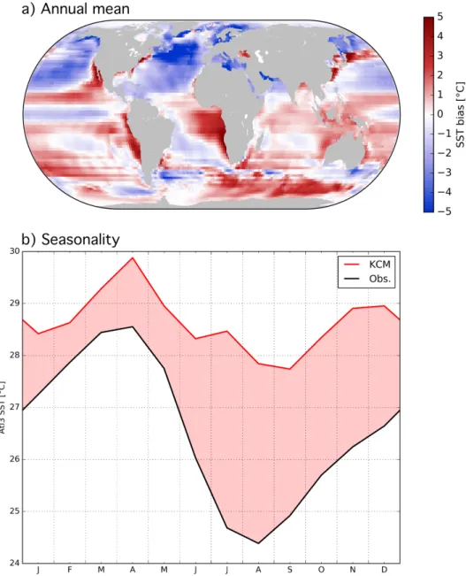
Climatological SST is a notoriously biased variable in CGCMs. Figure 1.4a shows

the annual mean SST bias of a suite of CGCMs that participated in the fifth phase of

the Coupled Model Intercomparison Project (CMIP5, Taylor, Stouffer, and Meehl, 2012).

Evidently, SST biases are abundant in the modelled ocean. Key features that are present

in virtually every current-generation CGCM are the severe warm biases in the western

subtropical ocean basins that reach annual mean amplitudes of up to

5

◦

C

(Richter and

Xie, 2008; Richter et al., 2014b). In the Atlantic, the spatial characteristics of the mean

bias are comparable to the structure of the Atlantic Niño. The bias is strongest off

the Namibian coast in the area of the Angola-Benguela front, with CMIP5-mean values

exceeding

5

◦

C. It stretches northwestward into the central equatorial Atlantic, producing

an equatorial warm bias with mean amplitudes of

1 −

2

◦

C. As in the real world, the mean state of a CGCM varies over the course of the year.

Consequently, a bias, too, can have a seasonal cycle. Figure 1.4b illustrates the seasonal

cycle of the Atlantic warm bias in a standard run of the Kiel Climate Model (KCM, Dippe,

Greatbatch, and Ding, 2018; Park et al., 2009) that consists of three ensemble members.

The bias is measured in the crucial, central equatorial region Atl3

3

_{. It is relatively small}

at the beginning of the year in the KCM, producing amplitudes that are hardly larger

(20)

Figure 1.4:

The equatorial Atlantic warm bias, diagnosed with respect to NOAA’s

ob-servational OISST dataset (Banzon et al., 2016; Reynolds et al., 2007) for the period

1982-2009. a) Annual mean SST bias of the ensemble mean of 33 CGCMs contributing

to CMIP5. b) Seasonal cycle of the SST bias in the Atlantic Atl3-region in a standard

integration of the Kiel Climate Model (KCM, red), relative to OISST (black). Both Figures

from Dippe et al. (2018).

tongue formation after May. In July and August, when the observed cold tongue is fully

developed, the KCM’s warm bias exceeds

3

◦

C. The KCM has failed to establish the

Atlantic cold tongue.

A host of research has addressed the dynamics of the equatorial Atlantic warm bias.

Because the atmosphere and the ocean are tightly coupled in the equatorial Atlantic,

too-warm SSTs are only one symptom of a coupled bias that links systematic errors in the

(21)

Many studies emphasise the importance of a pronounced westerly wind bias in the

western equatorial Atlantic for the development of the equatorial warm bias (Richter et

al., 2012). The westerly wind bias weakens the trade wind regime by substantially reducing

the strength of the easterly surface winds. When the bias is most pronounced in boreal

spring, it can reverse the direction of the zonal wind, turning easterly into weakly westerly

wind stress forcing. The reduced surface wind is in agreement with a systematic southward

displacement of the ITCZ (e.g. Doi et al., 2012; Richter et al., 2012; Siongco, Hohenegger,

and Stevens, 2015) and has been linked to a seesaw pattern of precipitation biases over

South America and Africa (C. Y. Chang et al., 2007; Patricola et al., 2012; Richter et

al., 2014b, 2012). Biased precipitation is related to systematic errors in tropical deep

convection, which in turn affects the gradient of surface pressure along the equator. The

equatorial wind field adapts to the anomalous surface pressure and as a result produces

the westerly wind bias.

The westerly wind bias is present in forced atmospheric simulations. It is an intrinsic

feature of most state-of-the-art atmosphere general circulation models (e.g. Harlaß, Latif,

and Park, 2017; Richter et al., 2014b).

In the strongly coupled equatorial Atlantic, the ocean adapts to the weak equatorial

winds and develops consistent oceanic biases. In agreement with reduced zonal wind stress

forcing, oceanic heat content is distributed more evenly along the equator, and the western

Atlantic warm pool is displaced towards the central ocean basin (C. Y. Chang et al., 2007;

Liu et al., 2013; Richter and Xie, 2008). The modelled thermocline is deeper than in

observations. Strengthening equatorial westerlies in late boreal spring are not sufficient

to shoal the thermocline in the central basin, and the initial cooling that sets off the

formation of Atlantic cold tongue cannot be established. The westerly wind bias keeps the

seasonal variations of surface wind stress in the western ocean basin from preconditioning

the central equatorial Atlantic for the formation of the cold tongue.

While the westerly wind bias is a key ingredient of the equatorial Atlantic warm bias,

the ocean models used in CGCMs are not free of error, either. For example, Grodsky et al.

(2012) show that forced ocean simulations in the tropical Atlantic are intrinsically biased

as well. Feedback processes between the atmosphere and the ocean amplify the intrinsic

biases of the stand-alone models and produce a severely biased system that is inconsistent

with the physical processes observed in the real world.

Based on a biased background that is unable to establish the Atlantic cold tongue,

past attempts to seasonally predict the variability of the Atlantic Niño have not been

successful (Hu and Huang, 2007; Kushnir et al., 2006; Stockdale, Balmaseda, and Vidard,

2006). While many studies have proposed methods to alleviate the equatorial Atlantic

warm bias in a physically consistent way (e.g. DeWitt, 2005; Harlaß, Latif, and Park,

(22)

1.5 Research questions of this thesis

A number of mechanisms have been proposed

to explain the Atlantic Niño. The

majority of existing research supports a dynamical Niño that is mainly driven by the

Bjerknes feedback (Burls et al., 2012; Carton et al., 1996; Keenlyside and Latif, 2007;

Zebiak, 1993). Nnamchi et al. (2015), on the other hand, argue that the Atlantic Niño

is a product of stochastic processes, discounting the role of dynamical ocean processes.

Chapter 2 seeks to reconcile these two approaches and raises the question

▶

How dynamical is the Atlantic Niño?

The dynamical interpretation of the Atlantic Niño relies on the framework of the

Bjerknes feedback, which also supports the growth of the Pacific Niño. Chapter 3 takes a

closer look at the Bjerknes feedbacks in the two basins and asks

▶

How symmetric are the Atlantic and Pacific Bjerknes feedbacks? Are

they stationary on decadal time scales?

Chapter 4 reviews the equatorial Atlantic warm bias and attempts to synthesise from

current research an answer to the question

▶

What drives the development of the equatorial Atlantic warm bias?

Last, Chapter 5 assesses the impact of the equatorial warm bias on the predictability

of the Atlantic Niño, asking

▶

Does the equatorial Atlantic warm bias affect the ability of a model to

predict the Atlantic Niño?

(23)

Chapter 2

On the Dynamics of the Atlantic

Niño

Previous studies on the mechanisms

generating and sustaining an Atlantic Niño

event have identified numerous processes, both dynamical and stochastic in nature. Here,

the relative contributions of ocean dynamics and residual stochastic processes to SST

variability in the equatorial Atlantic are assessed.

Citation:

Dippe, T., R. J. Greatbatch, and H. Ding (2018). “On the relationship

between Atlantic Niño variability and ocean dynamics”. In:

Climate Dynamics

51.1, pp. 597-612. DOI:

10.1007/s00382-017-3943-z

The candidate’s contributions to this manuscript are as follows. She

• Conceived the basic question that is discussed in the manuscript;

• Developed the statistical method to answer the research question;

• Performed all the analyses;

• Produced all the figures;

(24)

Clim Dyn

DOI 10.1007/s00382-017-3943-z

On the

relationship between

Atlantic Niño variability and

ocean

dynamics

Tina Dippe1 _{· Richard}_J._Greatbatch1,2_{· Hui}_Ding3

Received: 21 December 2016 / Accepted: 30 September 2017 © The Author(s) 2017. This article is an open access publication

operate in the model. Due to the small zonal extent of the equatorial Atlantic, the observed Bjerknes feedback acts quasi-instantaneously during the dynamically active periods of boreal summer and early boreal winter. Then, all elements of the observed Bjerknes feedback operate simultaneously. The model cannot reproduce this, although it hints at a better performance when using bias reduction.

1 Introduction

The Atlantic Niño is the dominant mode of interannual vari-ability in equatorial Atlantic sea surface temperature (SST). It modulates the seasonal development of the equatorial Atlantic cold tongue and peaks during May–August (Xie and Carton 2004). Similar to other modes of equatorial SST variability, it is the source of a number of teleconnections (e.g. Janicot et al. 1998; Mohino and Losada 2015), both regionally and globally. Through its close relationship with the Inter-Tropical Convergence Zone, it especially aﬀects rainfall variability over the surrounding continents, exerting an important socio-economic impact (Hirst and Hastenrath

1983).

Eﬀorts to simulate and predict equatorial Atlantic sea-sonal-to-interannual SST variability with state-of-the-art coupled global climate models (CGCMs) have not been very successful (Stockdale et al. 2006; Kushnir et al. 2006; Hu and Huang 2007). One reason for this is that most CGCMs suﬀer from a strong coupled bias in the tropical eastern Atlantic (e.g. Richter and Xie 2008; Grodsky et al. 2012; Wang et al. 2014). The SST signature of this bias stretches from the coast of Namibia and Angola into the equatorial Atlantic and is well established in the cold tongue region in the annual mean. Chang et al. (2007) and Richter et al. (2012) show that the equatorial SST bias is associated with

Abstract The Atlantic Niño is the dominant mode of inter-annual sea surface temperature (SST) variability in the east-ern equatorial Atlantic. Current coupled global climate mod-els struggle to reproduce its variability. This is thought to be partly related to an equatorial SST bias that inhibits summer cold tongue growth. Here, we address the question whether the equatorial SST bias affects the ability of a coupled global climate model to produce realistic dynamical SST variability. We assess this by decomposing SST variabil-ity into dynamical and stochastic components. To compare our model results with observations, we employ empirical linear models of dynamical SST that, based on the Bjerk-nes feedback, use the two predictors sea surface height and zonal surface wind. We find that observed dynamical SST variance shows a pronounced seasonal cycle. It peaks dur-ing the active phase of the Atlantic Niño and is then roughly 4–7 times larger than stochastic SST variance. This indicates that the Atlantic Niño is a dynamical phenomenon that is related to the Bjerknes feedback. In the coupled model, the SST bias suppresses the summer peak in dynamical SST variance. Bias reduction, however, improves the represen-tation of the seasonal cold tongue and enhances dynamical SST variability by supplying a background state that allows key feedbacks of the tropical ocean–atmosphere system to

*_{Tina Dippe}

[email protected]

1_{GEOMAR Helmholtz Centre for Ocean Research Kiel, Kiel,}

Germany

2_{Faculty of Mathematics and Natural Sciences, Christian}

Albrechts University, Kiel, Germany

3_{Cooperate Institute for Research in Environmental Sciences,}

University of Colorado and NOAA Earth Systems Research Laboratory, Boulder, USA

(25)

T. Dippe et al.

a fundamentally biased mean state in this region. The pool of warm surface waters that is observed in the western ocean basin shifts into the central ocean basin in biased simula-tions. The thermocline in the cold tongue region deep-ens, and upwelling is strongly reduced. The Atlantic cold tongue—the dominant feature of the SST seasonal cycle in the tropical Atlantic—cannot be established. Without a realistic cold tongue, however, CGCMs struggle to capture the observed Atlantic Niño, even in the presence of realistic forcing. Another factor that likely contributes to the models’ problems is that the dynamical nature of the Atlantic Niño is not yet fully understood.

While the name Atlantic “Niño” suggests a phenome-non that is essentially an Atlantic version of the Pacific El Niño-Southern Oscillation (ENSO), a number of diﬀerences exist between the two phenomena (e.g. Keenlyside and Latif

2007; Burls et al. 2011; Lübbecke and McPhaden 2012; Richter et al. 2013). Obvious are the diﬀerences in timing characteristics: Both positive and negative ENSO events generally peak in boreal winter and last for several months and in some cases even longer than a year. Atlantic Niño events on the other hand are phase-locked to boreal summer and rarely outlast a season. They have a smaller amplitude than their Pacific counterparts and appear to be the result of weaker atmosphere–ocean coupling. Additionally, while the canonical ENSO agrees with a self-sustained mode in the tropical Pacific, the Atlantic Niño requires external excita-tion (Zhu et al. 2012).

The dominant process that couples equatorial atmos-pheric and oceanic variability is the Bjerknes feedback (Bjerknes 1969). In a positive feedback, it relates SST and thermocline variability in the eastern ocean basin to zonal surface wind variability in the western ocean basin (u10) and lends growth to the Pacific (Bjerknes 1969) and Atlantic Niños (e.g. Keenlyside and Latif 2007; Burls et al. 2012; Lübbecke and McPhaden 2013; Deppenmeier et al. 2016). Traditionally, three elements of the Bjerknes feedback are considered when assessing the overall strength of the feed-back: (1) Eastern ocean basin SST anomalies force u10 anomalies in the western ocean basin, (2) u10 anomalies trigger a thermocline response across the basin that can be measured via thermocline variability in the eastern ocean basin, and (3) eastern basin thermocline anomalies amplify the initial SST anomaly. A closed Bjerknes feedback loop is present when all three elements of the Bjerknes feedback are active simultaneously.

Note, however, that the simplified Bjerknes feedback out-lined above is not the only process that acts in the equatorial oceans. Specifically, the “forcing direction” in the feedback elements (1)–(3) is not strict. In the closely coupled sys-tem of the equatorial oceans, wind variability in the

west-2006). Nevertheless, for the purpose of this study we will rely mainly on the dynamical framework of the simpli-fied Bjerknes feedback.

An important aspect of the Bjerknes feedback is that it must not necessarily act instantaneously. This means that the individual elements of the Bjerknes feedback may be delayed (note that this delay within the positive Bjerknes feedback is not identical with the range of delayed negative feedbacks discussed in Neelin et al. (1998) that ultimately stop anomaly growth in the eastern ocean basin during an El Niño or La Niña event). Physically, the delay within the elements of the positive Bjerknes feedback is due to the fact that information about anomalies on one side of the ocean basin need to be transmitted across the basin to be able to aﬀect the other side. In the atmosphere, this is done via rela-tively quick atmospheric adjustment to eastern ocean basin SST anomalies, which in turn produce anomalous zonal pressure gradients and result in western ocean basin zonal wind anomalies. In the ocean, zonal wind stress anomalies are translated into equatorial Kelvin waves (e.g. Dijkstra

2006). These Kelvin waves than travel westward across the ocean basin and feed the information about the wind vari-ability in the west to the eastern ocean basin. Depending on the width of the ocean basin, the Kelvin wave transmission can happen on a time scale on the order of months. In the tropical Atlantic, Keenlyside and Latif (2007) and Richter et al. (2013), among others, have shown that wind variabil-ity in the western ocean basin precedes SST variabilvariabil-ity in the eastern ocean basin by about 1 month in boreal spring. In the tropical Pacific, this delay is longer due to the larger basin size.

Returning to the dynamical nature of the Atlantic Niño in comparison to ENSO events, Burls et al. (2011) show that the Atlantic and Pacific Niños rely on the Bjerknes feed-back in subtly diﬀerent ways. The Pacific Niño generally is the result of a free mode of interannual variability that is driven by the Bjerknes feedback; interactions with the seasonal cycle occur, but do not dominate ENSO SST vari-ability. In the tropical Atlantic, on the other hand, the Bjerk-nes feedback is seasonally active (Richter 2016). It helps to develop the cold tongue and is involved in establishing the seasonal cycle. Burls et al. (2012) argue that the Atlantic Niño hence reflects a modulation of the seasonally active Bjerknes feedback instead of an independent mode of inter-annual variability.

Lastly, and in contrast to numerous studies that have provided evidence for a relationship between Atlantic Niño variability and the Atlantic Bjerknes feedback, Nnamchi et al. (2015, 2016) have proposed that the Atlantic Niño is essentially driven by stochastic processes in the atmosphere rather than by dynamical ocean processes that are

(26)

poten-On the relationship between Atlantic Niño variability and ocean dynamics

evidence for a significant stochastic component of Niño-like variability in the tropical Atlantic.

Here, we address two questions. First, do dynamical pro-cesses contribute to SST variability in the tropical Atlantic? Is there a seasonality to the ratio of dynamical and stochastic contributions? And second, does the presence of the SST bias—and hence the flawed mean state and missing summer cold tongue—aﬀect the models’ ability to accurately repro-duce the observed dynamical SST variance? To answer these questions, we use two assimilation runs of the Kiel Climate Model (KCM) as well as reanalysis data and decompose SST variance into a part that is due to dynamical processes in the ocean and a stochastic part that is driven by noise.

The rest of the paper is structured as follows: Sect. 2

sketches the Kiel Climate Model and the method that we used to produce our assimilation runs, Sect. 3 reviews the assimilation runs with respect to the impact of the equato-rial Atlantic SST bias. Section 4 presents our SST variance decomposition method; results for our assimilation runs and observations are compared in Sect. 5. Section 6 discusses the impact of lagged feedbacks on our results. A summary and discussion of the results is provided in Sect. 7.

2 Model and

methods

To compare our results with the evolution of the observed climate system, we use the ERA-Interim (Dee 2011) and the Archiving, Validation, and Interpretation of Satellite Oceanographic (AVISO) datasets. We find that diﬀerences between ERA-Interim SST and other SST datasets are neg-ligibly small. (Analysis results for alternative validation datasets such as the HadISST dataset (Rayner et al. 2003) are not shown. They diﬀer from the analysis with respect to ERA-Interim only in details.) Furthermore, our variance decomposition approach requires additional surface zonal wind (u10) and sea surface height (SSH) data. We use u10 provided by ERA-Interim for the period 1981–2012, and the AVISO monthly mean SSH anomaly dataset for the period 1993–2012. Throughout this study, we refer to ERA-Interim

(AVISO) when we discuss an “observed” feature of SST and u10 (SSH).

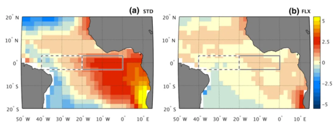
Figure 1 shows important regions for our study as boxes. Atl3 spans the region 3◦S–3◦N, 20◦W–0◦E and is the

Atlan-tic counterpart to the Pacific Nino3.4-region. It is the part of the equatorial Atlantic in which ocean–atmosphere cou-pling is most vigorous and that is hence used to assess SST variability associated with the Atlantic Niño. It is also the region in which the cold tongue is most pronounced in boreal summer. To the west of Atl3 is the western Atlantic region WAtl (3◦S–3◦N, 40– 20◦W). In terms of the Bjerknes

feedback, WAtl is crucial for the wind stress contributions to the feedback.

Model runs were performed with the Kiel Climate Model (KCM, Park et al. 2009), a coupled global climate model (CGCM). We used a low-resolution version of the KCM. The atmospheric component ECHAM5 (Roeckner et al.

2003) is run with 19 vertical levels in T31 horizontal resolu-tion. The ocean component of the NEMO model (Océan Par-allelisé Version 9, OPA9 Madec et al. 1998; Madec 2008) is run in the ORCA2-setup. ORCA2 has 31 vertical levels and an average horizontal resolution of 1.3◦. Towards the equa-tor, the horizontal resolution is refined to 0.5◦. The model

uses seasonally varying radiative forcing that corresponds to mid-twentieth century conditions. In particular, changes in greenhouse gas concentrations and aerosol loading are not considered.

We conducted two sets of experiments. The first set uses a standard version of the KCM (“STD”). The STD-SST cli-matology contains the SST bias in the southern subtropical Atlantic (Fig. 1), which is qualitatively comparable to the bias in other CGCMs (shown for example by Davey 2002; Richter and Xie 2008). The second experiment employs additional surface heat flux correction (“FLX”, see below for details) to reduce the SST bias. We run three and eight ensemble members for the STD and FLX experiments runs, respectively. All ensemble members use the same wind stress forcing (see below), but diﬀer in their initial condi-tions, which are taken from a control run at a time when the model is close to equilibrium.

Fig. 1 Annual mean SST bias relative to ERA-Interim SST in the a STD and b FLX assimila-tion runs in the tropical Atlan-tic. Positive values indicate that the model climatology is too warm. Solid (dashed) boxes show the Atl3 (WAtl) region

(27)

T. Dippe et al.

The STD and FLX experiments were run in partially coupled mode. Partial coupling is an assimilation technique that seeks to minimize the equatorial initialization shock in fully coupled hindcasts when they are started from partially coupled initial conditions (e.g. Ding et al. 2013; Thoma et al.

2015). In a partially coupled model the ocean and sea ice components are forced with observed wind stress anomalies that are added to the model’s monthly mean wind stress cli-matology. All other aspects of the model are identical to the fully coupled model. In particular, thermal coupling between the ocean and the atmosphere is preserved, and SST and the atmospheric wind field remain fully prognostic variables.

Surface heat flux correction is employed in the FLX experiment to reduce the SST bias of the KCM. To diag-nose the heat flux correction, we use the same methodol-ogy as Ding et al. (2015): During a control integration, we nudge the first ocean level of the model towards the monthly climatology of observed SST with a restoring time scale of 10 days. After 470 years, when the model has reached an equilibrium state, we continue our integration for another 70 years to diagnose the monthly climatological heat flux term that is associated with the SST restoring. This climatology of the “heat flux correction” is then added as a non-flow-interactive correction to the SST tendency while integrating the heat-flux corrected version of the KCM. For an overview of the performance of the two experiments in the equatorial Atlantic and the impact of the bias on the coupled system, refer to Sect. 3. Here, we note that Ding et al. (2015) showed a substantial improvement in the ability of the partially cou-pled model runs to reproduce observed SST variability in boreal summer in FLX compared to STD.

Monthly anomalies for the model integrations and valida-tion datasets are calculated by detrending the data via least-squares fitting, applied to each month separately. Note that we did not subtract the seasonal cycle from the monthly data prior to the detrending, since it did not yield qualitatively diﬀerent results. We chose this method to not only calculate our anomalies relative to a static seasonal cycle but allow the possibility that the seasonal cycle itself may vary (lin-early) on long time scales. The analysis period is 1981–2012 (1993–2012) for ERA-Interim and the KCM experiments (AVISO). For the KCM experiments, we detrend each ensemble member separately. The ensemble mean monthly anomaly is the average of the monthly anomalies of all ensemble members.

3 Impact of

the

coupled bias on

the

equatorial

Atlantic

In this section, we assess SST and zonal wind biases in the

experiments share their forcing of observed wind stress anomalies, the only diﬀerence between the ensemble means must be due to the bias correction in FLX. Hence, our analy-ses illustrate the impact that the bias has on the coupled equatorial system.

First, we assess the SST bias in STD and FLX. In the annual mean, the STD experiment shows the familiar pattern of the equatorial SST bias (Fig. 1a, 2.00 ◦C in Atl3). FLX

clearly reduces this bias (Fig. 1b, 0.29 ◦C in Atl3).

Addition-ally and in contrast to STD, FLX is able to produce a cold tongue similar to observations (Fig. 2). An interesting detail of Fig. 2 is that the STD experiment, too, simulates Atl3 cooling between April and May, but fails to intensify this cooling to establish the cold tongue from May onwards. In contrast, Atl3 cooling in FLX really only starts in May-June. Eﬀectively, cold tongue development in FLX lags behind observations by roughly 1 month (Fig. 2a). Nevertheless, heat flux correction clearly reduces the SST bias in the tropi-cal Atlantic (Fig. 2b).

Richter and Xie (2008) and Richter et al. (2012) have shown in diﬀerent CGCMs that the equatorial Atlantic SST bias is related to a bias in zonal surface wind in the west-ern equatorial Atlantic, which in turn can be traced back to precipitation deficiencies of the models. Based on obser-vations, Marin et al. (2009) argue that weak variability in WAtl zonal surface wind fails to precondition the basin-wide thermocline slope for the subsequent summer—the initial cooling of the cold tongue is hence weakened or delayed. In agreement with Richter et al. (2014a), a similar process could be at work in CGCMs: Spring zonal winds that are systematically too weak in the western equatorial Atlantic could inhibit seasonal thermocline shoaling in the eastern

Fig. 2 a Seasonal cycle of SST in Atl3 for (black) ERA-Interim, (red) STD, and (blue) FLX for 1981–2012. b Monthly mean bias of Atl3 SST for (red) STD and (blue) FLX

(28)

On the relationship between Atlantic Niño variability and ocean dynamics

Here, we demonstrate that the KCM, too, develops a zonal wind bias in boreal spring that is, however, largely independent of the SST bias in the eastern ocean basin. Figure 3 shows that zonal surface wind in WAtl is greatly reduced in boreal spring relative to ERA-Interim. Surpris-ingly, this behaviour is hardly altered qualitatively in the FLX experiment, indicating that the zonal wind bias depends only weakly on eastern basin SST in the model. In agree-ment with the recent findings of Richter et al. (2014b) and Harlaß et al. (2015) we suspect that the zonal wind bias is at least partly due to the insuﬃcient vertical resolution of the atmosphere model and related deficiencies in vertical momentum transport.

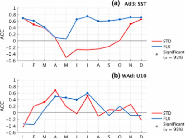
Additionally, we assess how the bias aﬀects the KCM’s ability to simulate observed SST and u10 variability. Fig-ure 4 shows, for each calendar month, the anomaly correla-tion coeﬃcient (ACC) between the ensemble means of the

partially coupled KCM assimilation runs and ERA-Interim. Again, because the FLX and STD experiments only diﬀer in whether they reduce the SST bias or not, diﬀerences in the “skill” of the assimilation runs to simulate the observed variability are due to the equatorial SST bias.

In agreement with Ding et al. (2015), bias reduction substantially increases the “skill” of the assimilation runs for boreal summer SST variability. This again supports the notion that the cold tongue is a crucial requirement for Atlantic Niño variability. Zonal wind variability, on the other hand, is only marginally improved by SST bias reduction in late boreal spring and early boreal summer.

An interesting aside with respect to the STD experiment is the strongly negative correlation coeﬃcient for modelled and ERA-Interim SST during May. The value is almost

−0.5, indicating a relationship that could be interesting to explore further. However, analysing in depth the physical processes that give rise to such an outstanding relationship in the biased experiment is not the scope of this paper and should be addressed in future research.

4 SST variance decomposition method

Figure 5 shows the SST variance in the tropical Atlantic and its seasonality. In ERA-Interim, Atl3 SST variance is subject to a well-defined seasonal cycle that peaks in May–July, con-sistent with the peak phase of the Atlantic Niño. In agree-ment with Okumura and Xie (2006) a secondary peak occurs early in boreal winter.

The KCM struggles to reproduce the observed SST vari-ance. While bias alleviation improves model performance, SST variance in FLX is too low and peaks 1 month late (Fig. 5). On the other hand, the STD experiment shows a seasonal cycle of SST variance that is almost the opposite of observations: Variance is high in boreal winter and decreases in boreal summer, reaching its minimum in July. Because the STD experiment is strongly biased in the tropical Atlantic (Figs. 1, 2), the cold tongue cannot develop in boreal sum-mer and cold tongue variability is not captured.

Fig. 3 Same as Fig. 2 but for zonal surface wind u10 in WAtl

Fig. 4 Monthly anomaly correlation coeﬃcients (ACCs) between ERA-Interim and the ensemble mean from the (red) STD and (blue) FLX experiments for a Atl3 SST and b WAtl u10 and the period 1981–2012

Fig. 5 Monthly SST variance in Atl3 for (black) ERA-Interim, (red) STD, and (blue) FLX