ePrints Soton
Copyright © and Moral Rights for this thesis are retained by the author and/or other
copyright owners. A copy can be downloaded for personal non-commercial
research or study, without prior permission or charge. This thesis cannot be
reproduced or quoted extensively from without first obtaining permission in writing
from the copyright holder/s. The content must not be changed in any way or sold
commercially in any format or medium without the formal permission of the
copyright holders.
When referring to this work, full bibliographic details including the author, title,
awarding institution and date of the thesis must be given e.g.
AUTHOR (year of submission) "Full thesis title", University of Southampton, name
of the University School or Department, PhD Thesis, pagination
PHYSICS AND ASTRONOMY
The Low Frequency Array and the
Transient and Variable Radio Sky
by
Martin Ellis Bell
Thesis for the degree of Doctor of Philosophy October 11, 2011
ABSTRACT
FACULTY OF PHYSICAL AND APPLIED SCIENCES PHYSICS AND ASTRONOMY
Doctor of Philosophy
THE LOW FREQUENCY ARRAY AND THE TRANSIENT AND VARIABLE RADIO SKY
by Martin Ellis Bell
This thesis addresses the topic of exploring and characterising the transient and variable radio sky, using both existing radio telescopes, and the next generation of radio facilities such as the Low Frequency Array (LOFAR). Studies of well known variable radio sources are presented in conjunction with blind searches of parame-ter space for unknown sources. Firstly, a three year campaign to monitor the low luminosity Active Galactic Nucleus NGC 7213 in the radio and X-ray bands is pre-sented. Cross-correlation functions are used to calculate a global time lag between inflow (X-ray) and outflow (radio) events. Through this work the previously es-tablished scaling relationship between core radio and X-ray luminosities and black hole mass, known as the ‘fundamental plane of black hole activity’ is also explored with respect to NGC 7213.
Secondly, the technical and algorithmic procedures to search for transient and variable radio sources within radio images is presented. These algorithms are in-tended for deployment on the LOFAR telescope, however, they are heavily tested in a blind survey using data obtained from the VLA archive. Through this work an upper limit on the rate of transient events on the sky at GHz frequencies is placed and compared with those found from other dedicated transient surveys.
Finally, the design, operation and data reduction procedure for the Low Fre-quency Array, which will revolutionise our understanding of low freFre-quency time domain astrophysics is explored. LOFAR commissioning observations are reduced and searched for transient and variable radio sources. The current quality of the calibration limits accurate variability studies, however, two unique LOFAR tran-sient candidates that are not present in known radio source catalogues are explored (including multi-wavelength followup observations).
In the conclusion to this thesis the parameter space that future radio telescopes may probe - including the potential rates of such events - is presented. At the nano-Jansky level up to 107 transients deg−2 yr−1 are predicted, which will form an unprecedented torrent of data, followup and unique physics to classify.
1 Introduction 1
1.1 Principles of radio astronomy . . . 1
1.1.1 Aperture synthesis . . . 5
1.2 The Low Frequency Array (LOFAR) . . . 9
1.3 The LOFAR Transients Key Science Project . . . 17
1.3.1 The LOFAR Radio Sky Monitor . . . 17
1.3.2 Commensal observing . . . 19
1.3.3 High time resolution mode . . . 19
1.3.4 The Transient Buffer Boards (TBBs) . . . 20
1.3.5 LOFAR imaging and transient detection algorithms . . . 20
2 Transient and Variable Radio Sources 21 2.1 Radio emission mechanisms . . . 21
2.1.1 Synchrotron . . . 21
2.1.2 Bremsstrahlung . . . 22
2.1.3 Black body . . . 23
2.1.4 Spectral lines . . . 24
2.1.5 Coherent emission mechanisms . . . 25
2.2 The transient radio universe . . . 25
2.2.1 Flare stars, active binaries, brown dwarfs and ultracool dwarfs 26 2.2.2 Neutron Stars . . . 27
2.2.3 Planets and exoplanets . . . 29
2.2.4 Intraday variability (IDV) and scintillation . . . 30
2.2.5 γ-Ray Bursts (GRBs) and Radio Supernovae (RSNe) . . . . 31
2.2.6 Active Galactic Nuclei (AGN) and X-ray binaries . . . 33
2.2.7 Gravitational wave events . . . 35
2.2.8 Future prospects . . . 36
2.3 Review of transient surveys to date. . . 36
2.4 This thesis . . . 38
3 X-ray and radio variability in the low-luminosity active galactic
nu-cleus NGC 7213 41
3.1 Introduction . . . 42
3.2 NGC 7213 Background . . . 44
3.3 Observations . . . 45
3.3.1 ATCA data analysis . . . 45
3.3.2 RXTE data analysis . . . 46
3.4 Results . . . 46
3.4.1 X-ray/radio light curves and cross-correlation . . . 46
3.4.2 Radio/radio cross-correlation . . . 52
3.4.3 X-ray/radio cross-correlation when flaring . . . 52
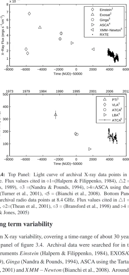
3.4.4 Long term variability . . . 53
3.4.5 Linear polarisation . . . 55
3.5 Discussion . . . 56
3.5.1 X-ray/radio jet connection . . . 56
3.5.2 The fundamental plane of black hole activity . . . 57
3.6 Conclusion . . . 64
4 Testing and refining the LOFAR transients detection pipeline 65 4.1 Introduction . . . 66
4.2 The prototype LOFAR transients detection pipeline . . . 66
4.2.1 Input: LOFAR images and metadata. . . 66
4.2.2 Source extraction . . . 68
4.2.3 Quality control . . . 69
4.2.4 MonetDB database and transient searches . . . 71
4.2.5 Source classification and alerts . . . 74
4.2.6 Monitoring . . . 75
4.3 Visualisation . . . 79
4.3.1 Interactive tools . . . 79
4.3.2 Webpages . . . 80
4.4 Considerations of single epoch transients . . . 83
4.5 Conclusion . . . 86
5 Archival radio transients 89 5.1 Testing the LOFAR transient detection pipeline on the Bower field . 89 5.1.1 Automated VLA reduction script . . . 90
5.1.2 Results and discussion . . . 92
5.2 The X-ray binary outburst of Swift J1753.3-0127 . . . . 98
5.3.1 VLA calibrator fields . . . 101
5.3.2 VLA data analysis . . . 103
5.4 Transient Search . . . 105
5.5 Results . . . 108
5.6 Snapshot rate upper limit . . . 109
5.7 Predictions for LOFAR . . . 115
5.8 Conclusion . . . 117
6 Blind searches for transients in LOFAR commissioning data 119 6.1 Introduction . . . 119
6.2 Test field B0329+54 . . . 119
6.2.1 The LOFAR Standard Imaging Pipeline (SIP) . . . 123
6.3 Imaging results and transient search . . . 128
6.4 Transient Candidate ILT J0320.3+5512 . . . 137
6.4.1 Multi-wavelength followup and catalogue search . . . 139
6.4.2 ILT J0320.3+5512 Discussion . . . 143
6.5 Transient Candidate ILT J0331.5+5712 . . . 146
6.5.1 Multi-wavelength followup and catalogue search . . . 146
6.5.2 ILT J0331.5+5712 Discussion . . . 150
6.6 Conclusion and Future Work . . . 153
7 Conclusion 155 7.1 Summary of thesis and future work . . . 155
7.2 Exploring SKA pathfinder parameter space . . . 157
7.3 A final remark . . . 164
APPENDICES
A Example Parsets 167
1.1 LOFAR telescope parameters . . . 14 1.2 Comparison of next generation radio telescopes survey speeds to a
sensitivity of 1µJy and 1 mJy . . . 16 3.1 Summary of the lag times which have been calculated using the
discrete correlation function . . . 48 3.2 Summary of archival observations found in the literature . . . 54 5.1 Summary of the Guassian fits produced from the LTraP compared
with those reported in Bower et al. (2007). . . 94 5.2 Summary of VLA calibrator observations used for an archival
tran-sient search. . . 102 5.3 Table of snapshot rates reported in the literature . . . 113 6.1 LOFAR observations of the B0329+54 field obtained for LOFAR
commissioning . . . 122 7.1 Predicted rates of radio transients for SKA pathfinder instruments . . 162
1.1 Example aperture synthesis arrays . . . 3
1.2 Field of view against 1 day sensitivity for current and future facilities 4 1.3 Example UV plots for the VLA and WSRT arrays . . . 6
1.4 Map showing the locations of the LOFAR international and core stations . . . 11
1.5 Example LBA and HBA antennas . . . 12
1.6 An example of the possible RSM configurations projected onto a coordinate grid. . . 18
2.1 A diagram depicting the evolution of the synchrotron shells within the jet of a black hole . . . 23
2.2 The radio evolution of the radio outburst of the X-ray binary XTE J0421+56, or CI Cam . . . 24
2.3 The intensity of the Lorimer burst as a function of radio frequency versus time . . . 29
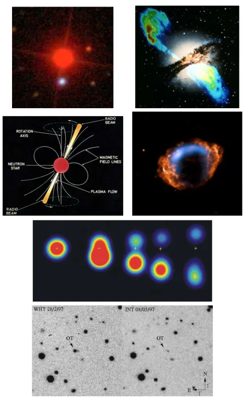
2.4 Examples of transient radio sources . . . 32
2.5 Examples of transient radio sources . . . 34
3.1 X-ray and radio lightcurves of NGC 7213 . . . 47
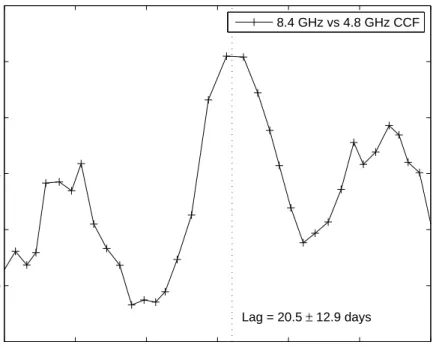
3.2 Discrete cross-correlation function (DCF) ray to 4.8 GHz and X-ray to 8.4 GHz . . . 50
3.3 The z-transformed discrete cross-correlation (ZDCF) function for the radio lightcurves . . . 51
3.4 Achival lightcurves of NGC 7213 . . . 53
3.5 The fundamental plane of black hole activity . . . 59
3.6 The fundamental plane using the KFC06 LLAGN sample only and updated FGR10 BHXRB sample . . . 60
3.7 Flare 1 radio data points at 4.8 GHz uncorrected for lag . . . 63
4.1 Flow diagram of the prototype LOFAR transients detection pipeline (LTraP) . . . 67
4.2 Flux per subband of the calibrator B0323.5+5510. . . 70
4.3 Example lightcurve of significantly variable source . . . 73 4.4 Example (simulated) lightcurves of transient behaviour that LTraP
currently struggles to correctly identify. . . 77 4.5 Example lightcurves of a wrongly classified single epoch transient . 78 4.6 Screenshot of prototype LOFAR transients visualisation tool . . . . 80 4.7 Example webpage for a transient source generated from the
visual-isation library. . . 82 4.8 Simulated detection of a transient where the transient duration is
less than the observation integration time . . . 85 4.9 Graph showing the burst flux SBas a function of burst time T needed
to produce a variety of final image fluxes SIm . . . 86
5.1 Flow diagram showing the automated VLA data reduction pipeline (version 1) . . . 92 5.2 Example images of Bower et al. (2007) field . . . 93 5.3 Image and lightcurve of the transient detection RT 1984-05-02 . . . 95 5.4 Image and lightcurve of the transient detection RT 1986-01-15 . . . 96 5.5 Image of the field containing RT 1999-05-04 made using the
auto-mated VLA pipeline . . . 97 5.6 Flow diagram showing the automated VLA data reduction pipeline
(version 2) . . . 99 5.7 Radio and X-ray lightcurves of the transient outburst of Swift
J1753.5-0127 . . . 100 5.8 Histogram showing the time difference between observations for an
archival VLA transient survey . . . 104 5.9 Flow diagram showing the automated VLA data reduction pipeline
(version 3) . . . 106 5.10 An example image of 3C48 at 4.8 GHz produced by the automated
VLA reduction pipeline . . . 107 5.11 Histogram showing the measured noise, calculated in the same
re-gion, for all VLA calibrator images . . . 110 5.12 Snapshot rate against flux density of transient detections reported in
the literature . . . 112 6.1 A map of the LOFAR station locations used in the commissioning
observation L21641 . . . 121 6.2 A schematic of the steps involved in the LOFAR standard imaging
6.3 Plots showing the effectiveness of the LOFAR automated RFI
flag-ging routines . . . 127
6.4 LOFAR image of the field 0329+54 taken on December 3rd 2010 . . 130
6.5 Lightcurve of the three unsubtracted LOFAR calibrators . . . 131
6.6 An image of the 2010-Dec-03 LOFAR observation . . . 132
6.7 An image of the 2010-Oct-10 LOFAR observation . . . 133
6.8 Comparison of the catalogued WENSS fluxes with the associated averaged LOFAR source fluxes . . . 134
6.9 A ‘zoom in’ to the edge of the LOFAR 2010-Dec-03 observation showing the postions of the WENSS sources . . . 135
6.10 The index of variability of all sources extracted in the B0329+54 images . . . 136
6.11 Images showing the transient candidate ILT J0320.3+5512 . . . 138
6.12 Lightcurve of ILT J0320.3+5512 . . . 140
6.13 Plot showing the positional offset of the Gaussian fits (including errors), to the transient candidate ILT J0320.3+5512 . . . 141
6.14 Optical image of the ILT J0320.3+5512 . . . 142
6.15 Spectral energy distribution of the candidate source . . . 144
6.16 Images of the transient candidate ILT J0331.5+5712 . . . 147
6.17 Lightcurve of the transient candidate ILT J0331.5+5712 . . . 148
6.18 Plot showing the positional offset of the Gaussian fits (including errors), to the transient candidate ILT J0331.5+5712 . . . 149
6.19 Optical image of the ILT J0331.5+5712 . . . 150
6.20 WSRT 1.4 GHz observation of the candidate transient . . . 151
6.21 Images of the transient candidate ILT J0331.5+5712 . . . 152
7.1 Predicted parameter space that the SKA and SKA pathfinders may explore . . . 159
7.2 Field of view against 1 day sensitivity for current and future facilities 160 7.3 An example Log N - Log S - Log t . . . 163
I, Martin Ellis Bell, declare that my thesis entitled The Low Frequency Array and
the Transient and Variable Radio Sky and the work presented in the thesis are both
my own, and have been generated by me as a result of my own original work, I confirm that:
• this work was done wholly or mainly while in candidature for a research degree at this University;
• where any part of this thesis has previously been submitted for a degree or any other qualification at this University or any other institution, this has been clearly stated;
• where I have consulted the published work of others, this is always clearly attributed;
• where I have quoted from the work of others, the source is always given. With the exception of such quotations, this thesis is entirely my own work;
• I have acknowledged all main sources of help;
• where the thesis is based on work done by myself jointly with others, I have made clear exactly what was done by others and what I have contributed myself;
• parts of this work have been published as:
⋆ Investigating the disc-jet coupling in accreting compact objects using the black hole candidate Swift J1753.5-0127, 2010, MNRAS, 406, 1471.
⋆ X-ray and radio variability in the low-luminosity active galactic nucleus NGC 7213, 2011, MNRAS, 411, 402.
⋆An automated archival VLA transients survey, 2011, MNRAS, 415, 2.
• parts of this work will soon be published as:
⋆Radio Transients: an antediluvian summary, Fender & Bell, 2011, Bulletin of the Astronomical Society of India, in prep.
Martin Ellis Bell, October 11, 2011
First and foremost I would like to thank Charli, my wonderful girlfriend. She has been there from the start of my University education 10 years ago - this thesis is dedicated to her. Secondly I would like to thank Rob Fender for giving me this opportunity, helping me through my studies, and drinking many beers - in may countries. Finally I would also like to thank my parents and family for their love and support and for staving off bankruptcy, ruin and hunger throughout my years as a student.
I would also like to thank my good friends (and bandmates) from Cornwall: Luke Toms, Mike Kitaruth, Phil Wilkes, Matt Truen, Niall Tomlinson and Ryan Jones. Thankyou for teaching me to not take myself too seriously (which wasn’t too difficult!). We will make some noise one last time at my viva party. I have met some really amazing people over the last four years in Southampton. My previous office mates and compadres who include Matthew Schurch, Mark Peacock, Simone Scaringi, Dave Russell, Omar Jamil, Sadie Jones, Grace O’Connor, Tony Wilkin-son, Seb Drave and Tana Joseph. Of which, many of them have forced me to party with them - a consequence of which being - that most Friday nights I had to sleep in the back of my car. I moved to Southampton shortly after this started to occur regularly. I would like to thank my current office mates Lee Townsend, Liz Bartlett (who shouts J¨agerbomb at me any time she is drunk), Dan Calvelo (let us not forget the portrait from Bangkok) and Dan Plant (for a bit of early morning egging).
I would also like to thank some of my great collaborators I have worked over the years. First of all Michael Wise and Sera Markoff, for giving me a roof over my head in Amsterdam and introducing me to a really fat cat (sorry Gingit). Also many thanks to Michael for putting up with my relative deterioration in mental health at a summer school (at an undisclosed astronomical facility). A further mention needs to be given to Sera, who helped relieve my T-shirts of sleeves - for reasons neither her or I can remember - at a late night bowling session in Dwingeloo. Also, Rob for taking a photo of the scene and showing it to everybody the next day. Many thanks to the LOFAR team: John Swinbank, Casey Law, James Miller-Jones, Bart Scheers, Ben Stappers, Evert Rol, Ralph Wijers, Thijs Cohen and Jason Hessels - I have enjoyed many a fine bottle of scotch with you all. A special thanks also to Jess Broderick for the countless conversations we have had about LOFAR data reduction over the last 18 months.
I also like to thank the staff at the University of Southampton. Specifically, Tom Maccarone and Phil Uttley for their help and support over the years. I would also like to thank the ‘girls’ from the school office: Mandy, Wendy, Kim, Hannah and Jan for the countless questions I have needed to ask regarding (usually) badly behaving students.
Merastawhye - Kernow bys Vyken
Martin Ellis Bell, October 11, 2011
investigate.
S
OPHOCLES,
C. 420 BCE
I don’t know how people have time to read books, I am
far too busy lying drunk face down in wet fields.
unbelievability of the thing, that I began to doubt the faith of my own eyes.
TYCHOBRAHE(1546 - 1601)
1
Introduction
1.1
Principles of radio astronomy
Since the serendipitous discovery of radio emission emanating from the Milky Way by Karl Jansky (1905-1950), radio astronomy has delivered paradigm shifting ad-vances in astrophysics. These include the discovery of the Cosmic Microwave Background radiation (CMB; Penzias & Wilson 1965), the Pulsar (Hewish et al., 1968), and the first binary Pulsar - which provided the most stringent test of General Relativity to date (Taylor et al., 1979). All three of these discoveries were awarded the Nobel prize. One of the most difficult challenges, which has and always will make radio astronomy a diffcult discipline, is manifested in the very nature of radio waves: wavelength. The typical radio wavelength is some million times greater than in the optical regime. Thus to achieve a radio image with the same resolution as the human eye (∼1 arcsec) we would need a radio telescope with a diameter of ∼1 kilometre, operating at a wavelength of 50cm (see Sir Martin Ryle’s Nobel Lecture 1974).
There were obviously technological challenges to building parabolic radio re-flectors of 1 km in diameter in the mid 20th Century and many still remain today. To reconcile the problem multiple (smaller) radio telescopes are placed some
tance apart (in arrays) and a technique called aperture synthesis (Ryle & Hewish, 1960) is used to make a ‘synthesised’ single telescope. The collecting area of the array is less than a completely filled aperture (resulting in lower sensitivity for such arrays), but the greatest angular resolution is dictated by the maximum baseline length. By utilising greater numbers of parabolic reflectors or dipole elements the telescope sensitivity can be improved.
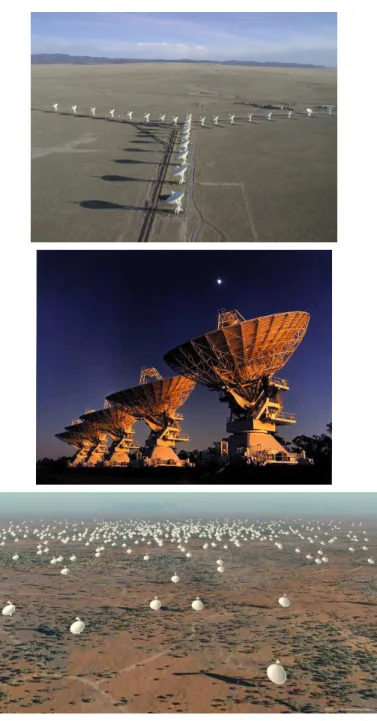
Radio interferometers that were constructed in the late 20th Century, such as the Westerbork Synthesis Radio Telescope (WSRT; Baars & Hooghoudt 1974), the Very Large Array (VLA; Hjellming & Bignell 1982), the Giant Metrewave Ra-dio Telescope (GMRT; Swarup 1990) and the Australian Telescope Compact Array (ATCA; Frater et al. 1992), use a small number (6 - 27) of parabolic reflector an-tennas. The VLA, ATCA and WSRT telescope diameters are∼ 25m, the GMRT uses 42m dishes. The next generation of radio telescopes many use may thousands of smaller (∼ 10m and less) parabolic reflectors, or dipole elements. See Figure 1.1 for photographs of the VLA (top panel), the ATCA (middle panel) and also an artists impression of the proposed Square Kilometer Array (SKA; bottom panel), which will potentially have a total collecting area of one square kilometre. In the parabolic case, decreasing the antenna diameter increases the field of view, while increasing the numbers of antennas and baseline length maximises the sensitivity and resolution. In the case of dipoles, the potential field of view is the whole sky, as they are omni-directional. They are also cheap to build, therefore many hundreds of thousands of antenna elements can be incorporated into an array. Figure 1.2 shows the field of view of current and future radio facilities, with respect to sensitivity. A defining characteristic of the future radio facilities is the instantaneous sensitiv-ity, and wide-field of view they can achieve. I will discuss some of these facilities further in later sections.
One of the major difficulties with ‘many element’ aperture synthesis is the trans-portation of vast quantities of data over large distances and also the computational power needed to produce images from the data. Thus the revolution, for radio as-tronomy, comes in the form of high speed optical fibre networks (either dedicated or over the internet) which are used for data transport; and the use of (what is considered at the time of writing) supercomputers for correlation and data reduc-tion. We are on the cusp of a major shift derived from these technological advances which may allow us to deliver Sir Martin Ryle’s one kilometre telescope (or larger). However, the next generation of radio telescopes will still rely on the principles of aperture synthesis.
Figure 1.1: Example aperture synthesis arrays. Top panel: The Very Large Array
(VLA) which consists of 27×25m dishes, with a maximum baseline length of
∼35km, located in New Mexico, USA. Middle panel: The Australia Telescope
Compact Array (ATCA) located in Narrabri, Australia, which contains 6×25m
dishes that can have a maximum baseline length of 6 km. Bottom panel: The proposed Square Kilometer Array (SKA) which may consist of many thousands of small parabolic reflectors and dipoles and will be located in either South Africa or Australia.
Figure 1.2: Field of View (FoV; deg2) against 1 day sensitivity (µJy right axis) for current facilities (small circles) and new facilities (large circles). The Aus-tralian Square Kilometre Array Pathfinder (ASKAP) and the Karoo Array Tele-scope (MeerKAT) are both GHz facilities which are in the early stages of con-struction in Australia and South Africa respectively. ASKAP will utilise phased
array feed technology to achieve a FoV of∼30 deg2, whilst MeerKAT will use a
single pixel feed to achieve a FoV∼0.5 deg2: both facilities will be fully
opera-tional ∼2014. APERture Tiles in Focus (APERTIF) is an upgrade to the WSRT
telescope which will increase the FoV to∼8 deg2(using phased array feeds), and
will be completed by 2013. SKA-SPF denotes the FoV and sensitivity of a single pixel SKA feed. SKA-PAF denotes a phased array feed, which has a wider FoV. Figure courtesy of R. Fender.
aperture synthesis, as this is fundamental to the science presented in this thesis. I will also explore how the next generation of radio telescopes, such as The LOw Frequency ARray (LOFAR; de Vos et al. 2009) will need to advance on the strate-gies developed for the older generation of radio instruments to achieve wide-field, high dynamic range imaging. It is not only a technological shift which will define this new generation of radio telescope: it is also the transformational science they will provide. In the context of this thesis, I will concentrate on time domain or ‘transient’ radio science. This introduction reviews the current state of the art of transient radio surveys and also explore examples of known and predicted transient radio sources. It also presents the design, construction and operation of the LOFAR telescope.
1.1.1
Aperture synthesis
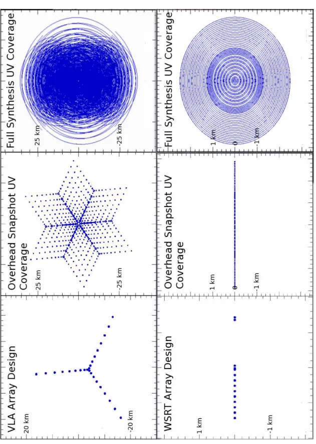
The principle of aperture synthesis relies heavily on the inverse Fourier transform. A large number of individual antennas (or telescopes) are separated by a variety of distances. The completeness of the synthesised aperture is dependent on the decli-nation of the source being observed, and the antenna locations as a function of time: these components define the uv plane. With a good distribution of antennas, short timescale observations can produce good images. Alternatively, a method that is more common for East - West type arrays is using the Earth’s rotation to synthesise a complete aperture. Both methods effectively measure Fourier components of the astronomical target source(s). The WSRT is an East - West array i.e. the anten-nas are positioned linearly in an East -West direction (see Figure 1.3). Therefore to achieve good spatial sensitivity, the Earth’s rotation must be used to sample a large number of Fourier components. The VLA is a ‘snapshot’ array whereby the antennas are positioned in a Y-shape (see Figure 1.3) which achieves much better instantaneous spatial sensitivity. The Earth’s rotation can still be used to fill in the VLA’s synthesised aperture further, however, good images can be produced in short timescales. Figure 1.3 shows the array layout of both the VLA and WSRT; also shown is the instantaneous overhead snapshot uv coverage and the full synthesis (12 hour) uv coverage for a source at δ =60◦. It can be seen that WSRT relies heavily on the Earth’s rotation to adequately fill in the uv plane, whist the VLA can achieve relatively good coverage in a short time.
The astronomical radio waves arriving at each different antenna are corrected for geometric delay (due to different path length differences). Then, for each antenna pair within the telescope, at each uv position and integration time unit, the amplitude (A) and phase (θ) of the correlated signal is measured. We can then use both A and θ to calculate the complex visibility V(u,v) =Aeiθ: which is equal to the 2D Fourier transform of the source sky function I(x,y)evaluated at each uv position. The full expression is shown in equation 1.1 below.
V(u,v) =
+∞ ZZ
−∞
I(x,y)e2πi(ux+vy)dx dy (1.1)
To characterise the target source well, we would want to sample as many visibili-ties as possible at different spacial frequencies. We can then find the sampled sky function I′(x,y)and produce an image by using the inverse Fourier transform:
Figure 1.3: Top panel: The array layout of the VLA (left) with the corresponding
overhead snapshot uv coverage (middle) and the full synthesis UV coverage for a
source atδ =60◦. Bottom panel: The array layout of the WSRT (left) with the
corresponding overhead snapshot uv coverage (middle) and the full synthesis UV
coverage for a source at δ =60◦. Figure modified from http://192.96.5.2/
I′(x,y) =
+∞ ZZ
−∞
V(u,v)e2πi(ux+vy)du dv (1.2)
Note, if the uv plane is completely sampled then I′(x,y)is the true sky function. If the uv plane is sparsely filled then we yield an approximation of the sky function. This approximation can also be characterised by using the convolution theorem:
I′(x,y) =B(x,y)∗I(x,y) (1.3)
B(x,y) is the Fourier transform of the uv function, which is typically referred to as the dirty beam. Equation 1.3 shows that what we are typically measuring with an interferometer, is the sky function I(x,y), convolved with the response of our instrument B(x,y).
The difficulty from this stage onwards is that we do not know the values of
V(u,v)for all possible uv components. There are a number of approaches to solving this problem. In one implementation, we can set all visibilities equal to zero where they have not been sampled, then perform the inverse Fourier transform to get a distorted image. We then use an approach called deconvolution which assumes that we have a number of point sources within our sky function. By assuming that these sources are point like, we can then deconvolve the effect of the dirty beam and hence ‘clean’ an image to reduce distortions (e.g. see H¨ogbom 1974, Clark 1980).
To further complicate the situation, we must undertake a set of tasks collectively referred to as calibration. The term calibration encompasses a large number of cor-rections that must be applied to the visibilities to produce an adequate image. These corrections must account for: perturbations in instrumental stability (system tem-perature), atmospheric transmission (e.g. phase calibration), positional/pointing ac-curacy, polarisation (including cross-polarisation leakage), absolute flux scale cali-bration, bandpass calicali-bration, bandwidth smearing and primary beam correction.
Typically for older interferometers, such as the VLA or ATCA, the calibration applied only makes approximations for some of the corrections described above. For example, a typical 1st generation calibration strategy is to measure the flux and phase of a nearby bright source, before and after the target observation. The derived calibration is then applied to the target source. This method relies on instrumental stability between the target and calibrator observations. A 2nd generation calibra-tion strategy, sometimes referred to as SELFCAL, is a closed-loop system which continuously updates the calibration as a function of time and is therefore less de-pendent on instrumental stability (see Noordam & Smirnov 2010 for a discussion
of calibration strategies). Some of the corrections described above (such as am-plitude and phase calibration) are degenerate moving away from the phase centre across the field of view. As discussed earlier the next generation of radio telescopes will potentially image very large fields of view, therefore a more complete descrip-tion of equadescrip-tion 1.1 must be implemented, which will incorporate 3rd generation calibration techniques.
The Radio Interferometer Measurement Equation (RIME) was first derived by Hamaker et al. (1996) and is further discussed in Smirnov (2011a,b,c). The RIME takes all the terms needed for calibration and represents them as Jones matrices. These Jones matrices fully map out the transmission of the electromagnetic wave (in polarisation, amplitude and phase) through the interferometer system. They form multiple simultaneous equations which must be solved to completely calibrate all the perturbations in the system. The calibration matrices are split into two types, direction dependent and direction independent. Direction dependent equations have typically been ignored for interferometers such as the VLA and ATCA, but must be used for calibrating wide-field instruments. The matrices are combined with equation 1.1 to form a complete measurement equation:
V(u,v) =Gp +∞ ZZ −∞ X(p,q)e2πi(ux+vy)dx dy Gq (1.4) where Xp,q=EpI(x,y)Eq (1.5)
I(x,y) is a 2 × 2 brightness matrix which characterises the polarised sky bright-ness as a function of direction (x,y). Ep and Eq represent a number of direction
dependent Jones matrices which contain the corrections needed for antennas p and
q. Gp and Gq represent the direction independent Jones matrices. If the telescope
only has a small field of view, Ep and Eq can be neglected and the measurement
equation returns to equation 1.3 - with the inclusion of the direction independent corrections Gp and Gq. The full implementation of RIME is computationally
ex-pensive and has probably slowed progress in radio astronomy. However, RIME is a complete description of the telescope system and must be considered when working with wide-field instruments.
The purpose of showing this theory is to place the technical work of this thesis in context. In this thesis I will use typical 1st and 2nd generation calibration and imaging techniques in Chapters 3 and 5. In Chapter 6 I will present the process of
producing wide-field images with LOFAR, for which direction dependent effects are apparent. A variety of new wide-field facilities will soon be available to sample the transient sky, and will make use of the techniques described above. In the radio band the Allen Telescope Array (ATA; Welch et al. 2009), the Murchison Wide Field Array (MWA; Lonsdale et al. 2009), the Long Wavelength Array (LWA; Ellingson et al. 2009) and LOFAR will soon begin or have already commenced operations. Other wide-field radio pathfinders such as the Karoo Array Telescope (MeerKAT; Booth et al. 2009) and the Australian Square Kilometre Array Pathfinder (ASKAP; Johnston et al. 2008) are also being developed on the road to the Square Kilometer Array (SKA; Rawlings & Schilizzi 2011). Transient studies are a key science goal for all of these facilities.
1.2
The Low Frequency Array (LOFAR)
The LOFAR telescope is an international project (led by The Netherlands) which utilises many low-cost dipole antenna elements (organised into stations) that are constructed at different locations across Europe. There are eight international LO-FAR stations located in the following countries: France (×1), Germany (×5), Swe-den (×1) and the United Kingdom (×1), see Figure 1.4 for a photograph of the UK Chilbolton station (left). There is a central ‘core’ located in The Netherlands which consists of 22 individual stations, see Figure 1.4 for a photograph (right). There are also 18 Dutch remote stations with baseline lengths<100 km (from the central core). The locations of the international and the Dutch core LOFAR sta-tions are shown in Figure 1.4. As LOFAR operates in the relatively unexplored low frequency regime, very long baseline lengths are needed to achieve good resolution. The LOFAR telescope design is a relatively unique concept as it does not use large steel dishes to focus radio waves, it uses many thousands of non-movable omni-directional dipole antennas, combined with the process of aperture synthesis and imaging. The concept of using dipoles in a telescope array is not so new. There has been a rich historical heritage in using dipoles and non-parabolic telescope de-sign in the past. For example Karl Jansky’s radio telescope used simple dipoles on a steerable platform (circa. 1930). Other instruments such as the Clark Lake Teepee-Tee Telescope and the Ukrainian T-shaped Radio Telescope (UTR-2) have, or still use, non-parabolic telescope design. The difference for LOFAR (and other instruments discussed below) is the inclusion of long baseline aperture synthesis and imaging. Many of the older generation instruments were not capable of
pro-ducing images or incorporating signals from antennas spaced on kilometre baseline lengths. Telescopes such as the MWA and LWA have also adopted a non-parabolic design, similar to LOFAR.
Each LOFAR international station typically consists of 96 low band dipole an-tennas, and 96 high band tiles. The Dutch stations can vary in size from a half to a quarter that of the international stations. Signal processing techniques are used to add phase delays in the signal path (between different dipole elements) to ‘steer’ the telescope beam to a region of the sky. This process is typically referred to as beamforming and the result is referred to as the station beam. Once a station has been phased together, the station beams from two different stations are correlated to provide the uv components described in section 1.1
There are two distinct types of antennas: the Low Band Antenna (LBA) shown on the top panel of Figure 1.5, which operate in the frequency range 10 to 90 MHz (but are mostly effective in the range 30 - 80 MHz); and the High Band Antenna (HBA) shown on the bottom panel of Figure 1.5, which operate from 110 to 250 MHz. The gap in observing frequency is due to the FM radio band, which will sat-urate all observations at those frequencies. The station design and subsequent beam forming of the LBA and HBA are slightly different. The HBA are arranged into tiles which consist of 16 folded dipoles arranged into 4×4 blocks. These 4×4 dipole blocks are then phased together using an analogue beam former at the tile level -which is referred to as the tile beam. This restricts the HBA field of view before the data have been digitised. The station beams are then formed digitally from the data stream received from the tiles. Note, there are 96 dipoles in an international LBA station and 96 tiles in the HBA. As each HBA tile consists of 16 dipoles, a total of 1536 dipoles are in fact present in the HBA station. The wavelength is smaller at the HBA frequency range than at the LBA range, therefore a larger number of dipoles can be packed together in a smaller space in the HBA. This increase in the number of dipoles comes with the consequence of increased data rates. The HBA dipoles are therefore phased together at the station level (using the analogue beam former) to reduce the data volume, which comes with the tradeoff of reducing the field of view.
The LBAs are arranged in a pseudorandom manner (within a station) and the signals are phased together digitally to form the station beam. Note, as there is no analogue beam former for the LBAs, they essentially view the whole sky all the time. Bright sources, such as Cassiopeia A (which are extremely bright at low frequencies∼kJy), are therefore always present in observations. Signal processing techniques must be used to subtract the effects of these bright sources to produce
Figure 1.4: Map showing the locations of the LOFAR international and core
sta-tions. A photograph is shown (left) of the recently constructed Chilbolton UK station (credit: LOFAR UK). The large circle represents the central core station, which comprises of a number of smaller individual stations. It also encompasses the Dutch remote stations which offer intermediate baseline lengths with respect to the core and international stations. A photograph is shown (right) of the central core station or ‘Superterp’ (credit: Astron).
Figure 1.5: Top panel: The first Low Band Antenna (LBA) to be constructed at
the LOFAR UK Chilbolton station. The antenna consists of a low noise amplifier mounted on a piece of tubing, which is secured via the XX and YY polarised dipole wires to a reflective ground plane (credit: LOFAR UK). Bottom panel: Two
High Band Antennas (HBA) which are typically deployed in 4×4 tiles within a
protective casing (credit: Astron).
adequate images.
The number of station beams formed by LOFAR is simply dictated by hardware and software constraints. For example one single station beam can be made with a bandwidth of 48 MHz, or up to 244 beams can be formed with a bandwidth of 48/244=0.2 MHz per-beam. All beam formed data collected via the stations is transported to a central processing hub in Groningen (shown on Figure 1.4 in blue) which utilises an IBM BlueGene/P supercomputer to produce the correlated visibil-ities. The data volumes are large; a 12 hour dataset with 25 stations using 1 second visibility averaging produces 15 TB of data. (McKean et al., 2011). Further de-tails of the design and signal processing of LOFAR see de Vos et al. (2009). A full description will also soon be available by Haarlem et al. (in prep).
Vos et al. 2009): σ =q W 2(2δνδt){Nc(NcS2−1)/2 core + NcNr ScoreSremote+ Nr(Nr−1)/2 S2 remote } (1.6)
Where σ denotes the noise measured in the final image (Jy). δν is the operating bandwidth (MHz). δt is the integration time (s). Nc is the number of core
sta-tions and Nr is the number of remote stations. Score and Sremote denote the system
equivalent flux densities (SEFDs) for the core and remote station respectively. W is a factor that accounts for the weighting scheme used in imaging (i.e. Natural, Robust etc.). At 150 MHz these values are Score =2.8 kJy, Sremote=1.4 kJy and
W =1.3. It should be noted that at the time of writing LOFAR was still being con-structed, therefore these values are subject to change. The reader should refer to de Vos (2009) for the predicted values of the SEFDs to be used in calculating the RMS noise. If only one type of station is used in the telescope setup then equation 1.7 (below) can be implemented.
σ =p Ssys
N(N−1)2δνδt (1.7)
Note, the calculation above only accounts for the thermal or theoretical noise limit, other factors such as dynamic range effects, bright sources in the side lobes, ambient temperature and RFI etc can play a role in increasing the noise. The resolution of LOFAR can be calculated using θ ∼ λ/D. Typical values of the sensitivity and
resolution as a function of frequency for the core and full LOFAR array are given in Table 1.1.
Due to LOFAR’s large field of view it is extremely well placed to survey large ar-eas of sky. This also makes LOFAR an excellent instrument to explore time domain radio astrophysics. To place the parameters summarised in Table 1.1 in context, I can compare these parameters with those expected for the Expanded Very Large Ar-ray (EVLA), which is an older generation interferometer with upgraded receivers. For the EVLA in A-configuration at 5 GHz, a field of view (FoV) of 0.07 deg2is re-alised. The sensitivity would beσEV LA=2.0µJy, in a 12 hour synthesis (assuming
a 1 GHz bandwidth). When compared with LOFAR a FoV of 28.8 deg2is achiev-able at 120 MHz with a sensitivity ofσLOF =110 µJy, using the core station only
in a 12 hour synthesis with 48 MHz bandwidth.
Although the LOFAR sensitivity does not seem as competitive as the EVLA, it is important to consider the spectral indexes of radio sources. For example, a typical synchrotron source withα=−0.7 (where Sv∝v+α) at 5 GHz would increase in flux
Table 1.1: Typical sensitivity (σ), resolution (θ) and field of view (Ω) as a func-tion of frequency, for the full array (including all internafunc-tional stafunc-tions) and the Dutch core station only. I assume the core consists of 22 stations, and the full array consists of 22 core and 26 remote stations. The sensitivities have been cal-culated using a bandwidth of 48 MHz. The field of view for each configuration
has been taken from the LOFAR technical website1. Note, the system equivalent
flux densities (SEFDs) used to calculate the parameters below are based on pre-dicted values. The sensitivities may therefore change (slightly) once the array is completed and the SEFD is properly parametrised.
Freq. σ1sec σ12hours σ1secs σ12hours θ θ Ω
(MHz) (mJy) (mJy) (mJy) (mJy) (′′) (′′) (deg2) Core Core Full Full Core Full Core
15 2980 14.3 1350 6.5 1650 48 1676
30 549.3 2.64 248.6 1.20 825 25 419
75 314.8 1.51 142.4 0.69 330 10 67
120 22.2 0.10 6.5 0.0314 206 6 28.8
200 22.8 0.11 6.6 0.0316 125 3.5 10.1
density by approximately an order of magnitude at 150 MHz. Therefore to achieve a source detection of 10σ with LOFAR with a source spectrum of α =−0.7, the equivalent detection with the EVLA would yield a 55σ detection, which is a factor of five improvement. However, in terms of FoV approximately 400 times the EVLA FoV can be imaged with LOFAR, in this example.
To further explore the competitiveness of LOFAR as a survey instrument in Table 1.2 I compare the survey speed of LOFAR with current and future instruments. The survey speed has been calculated using:
SS= 1
τ ×FoV[deg2hr−1] (1.8) Whereτ is the time taken to reach a given sensitivity in hours, and FoV is the field of view of the instrument. Each instrument will obviously reach a given sensitivity in a different amount of time, I therefore normalise each instrument by the amount of time taken to reach 1µJy and 1 mJy (see Table 1.2). I then calculate how many deg2(using the FoV) each instrument could survey in one hour, to define the survey speed in units of deg2hr−1. The LOFAR survey speed at 120 MHz using the full array is a factor of 100 faster than the VLA. However, some of the next generation of radio telescopes, such as the SKA, are extremely competitive. In this calculation I have used raw sensitivity only; as I demonstrated in the discussion earlier, a source with a typical spectral index ofα=−0.7 at 5 GHz would increase in flux by a factor of∼10 at 150 MHz. This corresponds to a factor of 100 increase in survey speed to detect a population of sources with this spectral index, because τ ∝1/(10σ)2.
The spectral index should be taken into account when comparing survey speeds at different wavelengths, as should the Log N - Log S of the known radio source population. I will return to a discussion of the known radio source and transient Log N - Log S later in this thesis. I will also discuss the concept of the transient source Log N - Log S - Log t, which is the time domain consideration of the standard Log N - Log S.
C h ap te r 1 . In tr o d u ct io n
Table 1.2: Comparison of next generation radio telescope survey speeds. σ12hours gives the sensitivity of each instrument in a 12 hour
integration. FoV gives the field of view of each instrument. τ gives the times needed to reach a sensitivity of 1 µJy and 1 mJy respectively. The survey speed gives the area of sky that could be surveyed per hour to a sensitivity of 1µJy or 1 mJy.
Telescope σ12hours FoV τ=1µJy Survey speed to 1µJy τ=1mJy Survey speed to 1 mJy
(µJy) (deg2) (hours) (deg2hr−1) (seconds) (deg2hr−1)
APERTIF (1.4 GHz) 10 8 1200 0.006 4.3 6666 SKA (Mid 1.4 GHz) 0.015 1 0.0027 370 9.7×10⁻⁶ 3.7×10⁸ SKA (Low<300MHz) 0.4 200 1.9 104 6.9×10⁻³ 1×10⁸ MeerKAT (1.4 GHz) 1.8 1 38 0.025 0.14 2.5×10⁴ ASKAP (1.4 GHz) 10.2 30 1248 0.024 4.5 2.4×10⁴ LOFAR (120 MHz Full) 31.4 28.8 1×10⁴ 0.0024 42.6 2.4×10³ LOFAR (30 MHz Full) 1200 419 1.7×10⁷ 2.4×10⁻⁵ 6.2×10⁴ 24.2 EVLA (5 GHz) 2.0 0.07 47 1.4×10⁻³ 0.17 1500 EVLA (74 MHz) 5000 322 3.3×10⁸ 2.0×10⁻¹⁰ 1.2×10⁶ 2.0×10⁻⁴ ATCA (5 GHz) 5.3 0.07 300 2.3×10⁻⁴ 1.0 2.3×10² GMRT (153 MHz) 15.5 10 2700 3.7×10⁻³ 9.7 3.7×10³ ATAa(1.4 GHz) 50 2.45 3.0×10⁴ 8.1×10⁻⁵ 100 81
1.3
The LOFAR Transients Key Science Project
There are six LOFAR key science projects: The Epoch of Reionisation, Extragalac-tic Surveys, Cosmic Rays, Solar Physics, Cosmic Magnetism, and Transients (see
http://www.lofar.org for further details). Each of these projects will benefit from dedicated observing time with LOFAR to achieve specific science goals. The Transients Key Science Project (TKSP; Fender et al. 2006) will aim to detect and monitor a broad range of transient astrophysical phenomena using LOFAR. The TKSP can be broadly split into two specialist areas: high time resolution and imag-ing. The high time resolution team (sometimes referred to as the Pulsar team) will probe transient phenomena with characteristic timescales 1µsec≤δt ≤1sec. The imaging team will probe transient phenomena with timescales 1sec≤δt to many
years. A variety of observational and transient detection techniques will be em-ployed by both teams, and I will explore these in detail in the following sections. In this thesis I am primarily concerned with image plane searches for transients, and the associated algorithmic detection techniques. The division between high time resolution and image plane searches is merely a division of observation and detection method. As I will discuss in greater detail later, certain classes of tran-sients could be prominent in both high time resolution and image plane searches. For example, a Pulsar would typically fall into the category of high time resolu-tion, however, pulsars are known to scintillate and should also be detected as highly variable sources in image plane searches.
1.3.1
The LOFAR Radio Sky Monitor
The Radio Sky Monitor (RSM) holds enormous scientific potential and will usher in a new era of all-sky radio astrophysics. The RSM will use a number of differ-ent overlapping beam configurations to tile up a large fraction of the sky to search for transients. This wide-field mode will open up the type of serendipitous discov-ery space that has been available to X-ray instruments, such as the All Sky Moni-tor (ASM) on the Rossi X-ray Timing Explorer (RXTE), for some time. Utilising LOFAR’s wide-field radio advantage, coupled with a potential daily monitoring ca-dence, the low-frequency radio parameter space can be explored and characterised. As discussed earlier, the available 48 MHz LOFAR bandwidth can be divided up to form a maximum of 244 beams. Figure 1.6 shows two possible configurations, at both 120 MHz (left panel) and 30 MHz (right panel) for surveying large areas of the sky. On the left panel, I show using black circles a Full Width Half Maximum
0:00:00.0 3:00:00.0 6:00:00.0 30:00:00.0 60:00:00.0 90:00:00.0 0:00:00.0 3:00:00.0 6:00:00.0 30:00:00.0 60:00:00.0 90:00:00.0
Figure 1.6: An example of the possible RSM configurations projected onto a
co-ordinate grid. Left panel: Black circles represent the FWHM of the HBA at 120
MHz (θ =5.3◦). The hexagonal pattern shows seven beams which overlap by
a factor of FWHM0.5, which yields a total FoV ∼0.12 steradians. The LOFAR
zenith track is also shown which can be tiled up using ∼30 overlapping beams.
Right panel: The same configuration but for the LBA at 30 MHz, each circle
rep-resents a FWHM ofθ =9.1◦. When tiled together using seven beams, a FoV of
∼0.35 steradians is realised. Approximately 20 LBA beams can tile up the entire
zenith.
(FWHM) of 5.3 degrees, which corresponds to the radius of the LOFAR HBA FoV at 120 MHz. By overlapping these fields of view by a factor of FWHM0.5 (see Condon et al. 1998), using seven overlapping beams, we can survey an area of sky
∼ 0.12 steradians (see hexagonal shape shown in Figure 1.6). Alternatively, in this figure I also show a zenith monitoring track. The LOFAR zenith is at∼54◦ North, by placing consecutive overlapping beams along this track, approximately 30 HBA beams can tile up the entire zenith. Observing at the zenith offers extra beam stability and optimises sensitivity (Fender et al., 2006). A combination of overlapping beams can be used to track the zenith fields for a given amount of time, using Earth’s rotation. The right panel of Figure 1.6 shows the same concept for the LBA at 30 MHz. At 30 MHz the LBA has a FWHM of 9.1 degrees; when this is tiled together with seven beams an area of 0.35 steradians is realised.
To best probe the parameter space available, images will be created on logarith-mically spaced ranges of timescales. The images will then be searched for tempo-ral changes in source brightness, and sources which are not found in current radio or multi-wavelength catalogues. Also, in a hybrid type observing mode, LOFAR could dedicate a large number of its beams to the RSM (including the zenith fields),
while a smaller number of beams perform daily monitoring of known radio transient sources, such as black hole X-ray binaries or active galactic nuclei.
1.3.2
Commensal observing
In parallel to dedicated TKSP observations, commensal observations can offer a large amount of data for transient searching. For example, the planned LOFAR Million Source Sky Survey (MS3) will survey the low frequency sky. The survey will not only offer a deep census of the LOFAR sky, but all data obtained through this survey can be searched for transient and variable radio sources, on a variety of timescales. The MS3survey will potentially be primarily concerned with producing one image of a given field over the total integration time (∼ 15 mins). The TKSP can divide this data up into (on the smallest scale) one second chunks to search for transients. In the future deeper surveys will be performed and the TKSP anticipate to search this data for transients. Furthermore, high time resolution data can be ob-tained simultaneous with imaging data, therefore all pulsars surveys (which are part of the TKSP mandate) are excellent candidates for commensal image plane transient searches. If a transient is detected via commensal observations, internal triggers can be used to re-point LOFAR, or via external triggers, to alert other facilities to obtain multi-wavelength followup.
1.3.3
High time resolution mode
High time resolution mode (sometimes referred to as Pulsar mode) will give LOFAR the capabilities of probing time-scales 1µsec≤δt≤1sec. The telescope setup, data reduction and data products are different from those produced in imaging mode. The data products will be time-series data rather than images. Specialist high time resolution algorithms will search for fast periodic and intermittent periodic signals, as well as single bursts. Also, known pulsars will be monitored to explore their low frequency profiles and properties.
Two different signal processing techniques, known as coherent and incoherent station addition, are used to combine the signals from different stations to form times-series data. The coherent station addition adds all the signals from the stations together, explicitly correcting for the phase difference between the station signals, from a particular direction. The incoherent addition combines the signals from the stations without correcting for the phase difference. There are trade offs to using each of these signal processing techniques. Coherent addition yields a better signal
to noise, but has a small field of view; this mode will mostly be used to monitor known pulsars due to it’s precision. Incoherent addition gains a larger field of view, but loses sensitivity, therefore this mode will be largely used for surveys. For further information on high time resolution mode and early results from observations of known pulsars see Stappers et al. (2011).
1.3.4
The Transient Buffer Boards (TBBs)
One of the unique properties of LOFAR is the Transient Buffer Boards (TBBs). The TBBs essentially consist of Random Access Memory (RAM) located at each station, that has the ability to record raw voltages for up to 1.3 seconds, at full bandwidth (Stappers et al., 2011). This gives LOFAR the ability to reprocess visi-bilities in greater detail after an event has occurred. The amount of time the TBBs can record is simply scaled by the amount of RAM available (and is upgradeable). Larger amounts of data can also be recorded if the bandwidth is reduced, which is defined by:
T =1.3 seconds×100 MHz
Br
(1.9)
Br is the reduced bandwidth (Stappers et al., 2011). Using a 4 MHz bandwidth,
which is potentially the amount which will be assigned to each RSM beam, 32.2 seconds of raw data may be recorded. This functionality is extremely useful for potentially receiving transients triggers from other instruments, or LOFAR itself, and beamforming at the region of interest to produce an image(s). See Singh et al. (2008) for further information on the TBBs. Note, this mode will primarily be used (at least initially) by the Cosmic Ray Key Science Project (see Falcke & Key Science Project (2007) for more details).
1.3.5
LOFAR imaging and transient detection algorithms
To produce images and detect transients on∼one second timescales, all data reduc-tion must be handled by dedicated pipelines. Automated data reducreduc-tion pipelines, for both imaging and transient detection, are currently in a state of heavy testing and commissioning. Chapter 4 describes in detail the LOFAR transient detection pipeline (LTraP) and the testing that has been conducted on the datasets described in this thesis. Chapter 6 describes the LOFAR standard imaging pipeline (SIP), and the application of the LTraP to LOFAR commissioning data.
HUNTERS. THOMPSON(1937 - 2005)
2
Transient and Variable Radio Sources
In this chapter I will review some of the prominent radio emission mechanisms, as they are fundamental to the science presented in this thesis. I will also review the types of known transient and variable radio sources. In the conclusion to this chapter I will review the current state of the art of transient radio surveys.
2.1
Radio emission mechanisms
2.1.1
Synchrotron
Synchrotron radiation is produced by the acceleration of electrons (or positrons) in a helical path due to magnetic field lines. The velocity of the spiralling electrons is relativistic. Synchrotron is closely related to cyclotron radiation, where the velocity of the spiralling electrons is non-relativistic, and also gyro-synchrotron where the velocity is mildly relativistic.
The spectrum of a synchrotron source is characterised by the underlying electron population. For the non-thermal case, the electron population can be described by a power-law distribution of electron energies i.e. N(E) =N0E−δ, then Sν ∝
ν−δ−1
2 (where Sv is the flux density in Janskys). This typically results in optically
thin spectrums of α ∼ −0.7 (where Sν ∝ν+α). Synchrotron emission can also
be absorbed, which results in a turnover of the spectrum withα ∼+2.5 at lower frequencies, for the non-thermal case. If the distribution of electron energies can be described as a thermal distribution, then the resulting spectrum at low frequencies yieldsα ∼+2 (further discussion will follow on thermal radiation). The peak flux of the radio emission is found at the frequency at which the emission switches from optically thick to thin.
Furthermore, the electron populations and the environments in which synchrotron radiation is produced can evolve. For example, in the radio emission produced by an expanding shell of plasma in the jet of a black hole (either an X-ray binary or active galactic nuclei), the electron population evolves from being dense to less-dense, as a function of time. Other factors such as changes in the magnitude of the magnetic field also affect the evolution of emission as a function of time (see van der Laan 1966 for further details). Figure 2.1 shows a simplified cartoon of this physical process. At a given frequency the shell of material will intially be optically thick (which will yield a spectrum of α ∼+2.5 in the non-thermal case). As the shell expands the flux rises as the shell becomes optically thin (α ∼ −0.7). This process is repeated at each different observing frequency. In active galactic nuclei and X-ray binaries the broad-band radio emission can commonly be described as flat spectrum (α ∼0). If we sum up all the synchrotron peaks (over a range of fre-quencies) we arrive at a flat spectrum (see Figure 2.1). In this simple model, I have ignored the consequence of ‘shocks’. I will return to this topic including a further discusion on jets in active galactic nuclei and X-ray binaries in Chapter 3.
To further demonstrate the model, Figure 2.2 shows lightcurves at a number of different frequencies, of an outburst from the X-ray binary XTE J0421+56, or CI Cam (see Belloni et al. 1999 and Fender et al. 2006). At the early stages the out-burst of the source has already peaked at higher frequencies. The lower frequency emission, specifically 0.33 GHz, starts to rise later due to the delay time for the expanding synchrotron shell to become optically thin at lower frequencies. At all frequencies, the decay of the emission (after the peak) is due to adiabatic expansion losses as the ejecta expands.
2.1.2
Bremsstrahlung
Bremsstrahlung emission (sometimes referred to as free-free emission) results from the acceleration of electrons within a plasma. Electrons are deflected by the ionised charge of a heavier ion and the resulting change in energy releases radiation. The resulting spectrum at high (radio) frequencies is relatively flat, then moving to low
Figure 2.1: A diagram depicting the evolution of the synchrotron shells within the
jet of a black hole. At a given frequency, as the shell expands, the radio emission will rise whilst the spectral index evolves from optically thick to thin. The summa-tion of the spectra over a broad frequency range, typically results in a flat spectrum. This model does not consider ‘shocks’ within the jet which will be discussed later in this thesis.
frequencies there is a turnover after which the spectrum is described by α = +2. Bremsstrahlung is very similar to synchrotron radiation, the difference being that synchrotron requires an ambient magnetic field: Bremsstrahlung utilises a charged plasma. Bremsstrahlung is therefore common in hot ionised environments, such as the hot intra-cluster gas of galaxy clusters.
2.1.3
Black body
Black body radiation arises from the oscillations of charged particles within an ob-ject. The flux density of a black body source increases with λ−2 (in the Raleigh-Jeans approximation), which yields a spectrum of α = +2. Most astronomical sources emit via the black body process and it is also observed whenever a thermal population of electrons (or protons) is optically thick (e.g. thermal synchrotron). The quiet sun, the moon and the cosmic microwave background radiation are ex-amples of black body emitters.
Figure 2.2: The radio evolution of the radio outburst of the X-ray binary XTE
J0421+56, or CI Cam. Observations of the source were conducted with the Ryle Telescope (15 GHz), the Green Bank Interferometer (2 and 8 GHZ) and the WSRT (0.8 and 0.33 GHz). The lightcurves show the late arrival time of the lower frequency (0.33 GHz) synchrotron emission. Figure and description taken from Fender et al. (2006).
2.1.4
Spectral lines
Spectral line processes are common across the electromagnetic spectrum. One of the most prominent and abundant spectral line processes in the radio regime, is the 21cm line. The 21cm line arises from a hyperfine spin-flip transition in neutral hydrogen, resulting in the release of a photon at 21cm, or 1.4 GHz. This type of radiation is produced at a discrete wavelength, therefore it can also be used to measure velocities using Doppler shifts. The 21cm has been used to map galactic rotation with our galaxy and others. It is also a potential probe of cosmology, a highly red-shifted 21cm line, at the time of the epoch of reionisation, would emit at a frequency<200 MHz. The LOFAR Epoch of Reionisation Key Project hope to study the density, temperature and velocity profiles of the heavily shifted 21cm line to learn more about the early universe.
2.1.5
Coherent emission mechanisms
The electron cyclotron maser is one example of a coherent radio emission mech-anism. Electrons are accelerated along magnetic field lines (typically in a plane-tary or solar environment), these electrons then produce photons via the cyclotron process. The cyclotron photons are then subsequently amplified by the maser (Mi-crowave Amplification through Stimulated Emission of Radiation) process. This bulk flow of electrons provides a population inversion in the electron distribution, which provides a ‘pump’ for the maser. The input photons stimulate greater num-bers of photons to be produced, and provides an amplification of the original cy-clotron radiation. The photons emitted by the maser process have the same (or similar) properties to the input photons, and since all photons are travelling in the same direction, they appear to come from a very compact region. The brightness temperature of a source is inversely proportional to the source size, therefore elec-tron cycloelec-tron masers (and coherent sources in general) have been shown to have extremely high brightness temperatures. Also, this type of emission has been shown to have high degrees of circular polarisation. Other types of coherent process exist which follow a similar theme to the electron cyclotron maser i.e. bulk flow of elec-trons - for further information on coherent processes see Dulk (1985). In the next section I will discuss the known types of transient radio sources and explore which emission mechanisms dominate.
2.2
The transient radio universe
The scope and depth of transient radio science is vast: by utilising the time domain we can gain unique insight into such objects as neutron stars and white dwarfs in binary systems, relativistic accretion and consequent jet launch around black holes, distant gamma-ray burst afterglows, supernovae and active galactic nuclei (AGN), to name a few. The distances to these objects, as well as the timescale for transient behaviour, varies dramatically. For example, giant kilo-Jansky micro-second radio pulses have been observed from the relatively nearby Crab Pulsar (e.g. see Bhat et al. 2008). In contrast, month timescale (and longer) variations are commonly observed in the radio emission produced by powerful jets driven by accretion onto super-massive black holes in distant AGN (Aller et al. 1985; de Vries et al. 2004; Bell et al. 2010; Jones et al. 2010). Through studying the transient and variable nature of these exotic and energetic objects, we obtain an unprecedented laboratory to probe extreme physics, on a variety of distance scales and in a number of different
environments. I will comment further on some of the broader scientific motivation to studying transients later in this chapter.
This thesis is concerned with the search, detection and scientific interpretation of transient and variable radio sources at both MHz and GHz frequencies. I will therefore review some of the known and predicted types of transient radio sources at both frequencies. I will put an emphasis on the expected differences between GHz and MHz populations (if appropriate), and also the typical timescales for tran-sient behaviour and expected flux densities.
2.2.1
Flare stars, active binaries, brown dwarfs and ultracool
dwarfs
Flare stars are typically late type stars (often referred to as dM or dMe stars; Bastian 1990) that undergo transient outbursts which increase the flux density by a factor of
∼500 (from mJy quiescent levels), at a range or radio frequencies (Strassmeier et al., 1993). The outbursts are often characterised at both MHz and GHz frequencies by: (i) a high degree (up to 100%) of circular polarisation (Jackson et al. 1989; Lang et al. 1983; Gudel et al. 1989); (ii) a high spectral index, typicallyα ∼ −2.5 (Lovell 1969; Spangler et al. 1974); (iii) high brightness temperatures, typically
Tb>1012K (Lovell 1969; Spangler & Moffett 1976); (v) bursts that can last from
tens of seconds to tens of minutes (Bastian 1990), sometimes up to days (Kundu et al. 1988; Slee et al. 2003). Due to the high brightness temperatures, steep spectral index and short timescale of variability a coherent emission mechanism is favoured over gyro-synchrotron<∼5 GHz. Above 5 GHz gyro-synchrotron can not be ruled out because the brightness temperature does not exceed TB=1012. A sub-divsion
of the flare star class incorporates active binaries (RS CVn and BY Dra Binaries) which share similar characteristics to standard flare stars (see Mutel & Weisberg 1978; Fix et al. 1980; van den Oord & de Bruyn 1994 and references therein). Based on the flare star radio burst statistics of Abada-Simon & Aubier (1997) and subsequent interpolation by Fender1 et al. (2007) to LOFAR considerations, flare stars will be abundant in routine monitoring with LOFAR. Due to LOFARs one second cadence and wide-field of view, a broadband census of nearby flare star activity can achieved.
Brown dwarfs are the smaller main sequence ‘non-starter’ cousins of flare stars; they are distinguished from planets via their ability to burn deuterium. Less is