Bootstrap inference for conditional risk measures

Bootstrap inference for conditional risk measures

Citation for published version (APA):

Heinemann, A. M. (2019). Bootstrap inference for conditional risk measures. Maastricht: ProefschriftMaken Maastricht. https://doi.org/10.26481/dis.20190620ah

Document status and date:

Published: 01/01/2019

DOI:

10.26481/dis.20190620ah

Document Version:

Publisher's PDF, also known as Version of record

Please check the document version of this publication:

• A submitted manuscript is the version of the article upon submission and before peer-review. There can be important differences between the submitted version and the official published version of record. People interested in the research are advised to contact the author for the final version of the publication, or visit the DOI to the publisher's website.

• The final author version and the galley proof are versions of the publication after peer review.

• The final published version features the final layout of the paper including the volume, issue and page numbers.

Link to publication

General rights

Copyright and moral rights for the publications made accessible in the public portal are retained by the authors and/or other copyright owners and it is a condition of accessing publications that users recognise and abide by the legal requirements associated with these rights.

• Users may download and print one copy of any publication from the public portal for the purpose of private study or research. • You may not further distribute the material or use it for any profit-making activity or commercial gain

• You may freely distribute the URL identifying the publication in the public portal.

If the publication is distributed under the terms of Article 25fa of the Dutch Copyright Act, indicated by the “Taverne” license above, please follow below link for the End User Agreement:

www.umlib.nl/taverne-license Take down policy

If you believe that this document breaches copyright please contact us at:

[email protected]

providing details and we will investigate your claim.

Bootstrap Inference for Conditional Risk

Measures

All rights reserved. No part of this publication may be reproduced, stored in a retrieval system, or transmitted in any form, or by any means, electronic, mechan-ical, photocopying, recording or otherwise, without the prior permission in writing from the author.

This book was typeset by the author using LA_TEX.

Published by ProefschriftMaken|| www.proefschriftmaken.nl ISBN: 978 94 6380 372 4

Bootstrap Inference for Conditional Risk

Measures

DISSERTATION

to obtain the degree of Doctor at Maastricht University,

on the authority of the Rector Magnificus, Prof. dr. Rianne M. Letschert,

in accordance with the decision of the Board of Deans, to be defended in public

on Thursday, 20 June, 2019 at 16.00 o’clock

by

Prof. dr. F.C. Palm

Co-Supervisors Dr. E.A. Beutner

Dr. S.J.M. Smeekes

Assessment Committee Prof. dr. A.W. Hecq (Chair)

Dr. N. Bast¨urk

Prof. dr. G. Cavaliere, University of Bologna, Italy

Prof. dr. C. Francq, CREST, Paris, France

Prof. dr. P.C. Schotman

This research was financially supported by The Netherlands Organisation for Scientific Research (NWO).

Acknowledgements

“You cannot connect the dots looking forward, you can only connect them looking backwards.”

Looking backwards, the starting point of my academic journey is a letter from Maastricht University, back in July 2010, congratulating me on the successful admission to theInternational Business program. I soon came to know that my primary study choice International Business Economics belongs to Economics

track. Misled by the ambiguous naming, I retrospectively thank the admission office for not allowing me to switch toEconomics. Acting by necessity, I switched toEconometrics and Operations Research instead – a decision I have never regret ever since. Nine years of intensive studies followed. Having reached the mountain’s top – my PhD defense – I would like to thank several people in particular, who accompanied me along the way.

First of all, I am greatly indebted to my supervisors and mentors Eric Beutner and Stephan Smeekes. It truly has been a privilege to work with and learn from the both of them. I consider myself extremely lucky to have not only one but two supervisors, who care so much about my work and are approachable anytime. Eric, I especially would like to thank you for your encouragement and for the numerous counter-examples invalidating former versions of the proofs. Stephan, I benefited a lot from your constructive remarks and bootstrap insights. In addition, I owe my promoter Franz Palm a debt of gratitude for reading several drafts and providing comments that greatly improved the work presented herein.

Further, I would like to thank the reading committee for taking the time to carefully evaluate and approve my thesis manuscript. In particular, I need to mention Christian Francq; he and Jean-Michel Zako¨ıan gave me a warm welcome at CREST, Paris, where I spent a fantastic time as a visiting researcher. Merci!

I hope we find the time to collaborate more in the future. A special thanks also goes to my former supervisor and friend Dante Amengual, who guided me through the reviewing process of theJournal of Applied Econometricsand who has a great share in publishing my first article. Muchas gracias!

Let me turn the attention to my paranymphs, Sean and Rasmus, who shared with me the up’s and down’s of the PhD. I cannot put in words how grateful I am for your pure friendship and the daily distractions. Sean, I already miss your infectious laughter and the inspiring voice messages after midnight. Rasmus, my Swedish friend, I highly appreciate your spontaneity and your sense of humor; sharing an office with you for over three years was a terrific experience. I also would like to thank Anne Balter and Farzaneh Rajabi Ghamchi for the wonderful atmosphere in office at the early and the final stage of my PhD.

A warm word of thanks goes to Yolanda Paulissen and Karin van den Boorn who facilitated my research activity by taking most of the administrative burden upon themselves. Van haarte bedankt! I also send my appreciation to my other colleagues, especially those who contributed to the legendary atmosphere on the 4th floor at SBE:

I express my gratitude to Peter Thesling, Frank Bosserhoff and Florentijn Hogerwerf for agezellige tijd and Jos´e Jimenez, Andreas Stegmann and Diego As-torga for the nice company and a great student time. Outside the academic circle I can always count on my lifelong friends Fabian Ziehms and Matthias Sch¨onfeld. You are the best! I also cannot get around to thank Alix Greiber, who guided me back to Maastricht. The Maashattan experience would not have been the same without Manos. Nine generations of Manos are simply too many to mention every single person, but I will never forget the memorable handball tournaments and member weekends.

Of course, I would like to acknowledge my family, the anchor in my life. Mama, thank you for the constant support over all these years and for always believing in me. Papa, my sincere apologies: you tried so hard to talk me out of mathematics, however ein Apfel f¨allt nicht weit vom Stamm.1 _{Special credits also go to my}

sisters Isabel, Kathi and Sarah. And I thank my penfriend Fabian, my princess Julia and my godchild Emil for being so adorable. Saving the best for last: Suus, I am truly blessed to have you in my life. Thank you for your patience and all the distracting smiles during stressful times.

Alexander Heinemann Maastricht, January 2019

Contents

“I was still a couple of miles above the clouds when it broke, and with such violence I fell to the ground that I found myself stunned, and in a hole nine fathoms under the grass, when I recovered, hardly knowing how to get out again. Looking down, I observed that I had on a pair of boots with except-ionally sturdy straps. Grasping them firmly, I pulled with all my might. Soon I had hoist myself to the top and stepped out on terra firma without further ado.”

Contents

Contents xi

1 Introduction 1

1.1 Risk Measures . . . 3

1.2 Classical Asymptotic vs. Bootstrap Inference . . . 4

1.3 Temporal Dependence . . . 7

1.4 Contribution and Outline of the Thesis . . . 8

2 A Justification of Conditional Confidence Intervals 11 2.1 Introduction . . . 12

2.2 General Setup . . . 14

2.2.1 The General Prediction Function . . . 14

2.2.2 Argument of Two Independent Processes . . . 21

2.2.3 Sample-split Estimation . . . 22

2.3 Asymptotic Justification . . . 24

2.3.1 Merging . . . 24

2.3.2 Merging of 2IP and SPL in Probability . . . 26

2.3.3 Interval Construction . . . 29

2.3.4 Interval Construction Under Normality . . . 32

2.4 Prediction Intervals . . . 34

2.5 Conclusion . . . 36

2.A Lemmas and Proofs of Theorems . . . 38

2.A.1 Lemmas . . . 38

2.A.2 Proofs of Theorems. . . 40

2.B Additional Proofs . . . 46

2.B.1 Proofs of Lemmas . . . 46

2.B.2 Proofs of Corollaries . . . 54

3.1 Introduction . . . 58

3.2 General Framework . . . 59

3.3 Conditional Mean in an AR(1) . . . 60

3.3.1 Model Description . . . 60

3.3.2 Estimation . . . 61

3.3.3 Mapping . . . 61

3.3.4 Verification of Assumptions . . . 61

3.4 Conditional Variance in a GARCH(1,1) . . . 64

3.4.1 Model Description . . . 64

3.4.2 Estimation . . . 65

3.4.3 Mapping . . . 66

3.4.4 Verification of Assumptions . . . 67

3.5 Conditional Mean in an ARMA(1,1) . . . 72

3.5.1 Model Description . . . 72

3.5.2 Estimation . . . 73

3.5.3 Mapping . . . 74

3.5.4 Verification of Assumptions . . . 75

3.6 Conditional Volatility in a T-GARCH(1,1) . . . 81

3.6.1 Model Description . . . 81

3.6.2 Estimation . . . 82

3.6.3 Mapping . . . 83

3.6.4 Verification of Assumptions . . . 84

3.7 Concluding Remarks . . . 90

4 A Residual Bootstrap for Conditional Value-at-Risk 93 4.1 Introduction . . . 94

4.2 Model . . . 96

4.3 Estimation . . . 97

Contents

4.4.1 Fixed-design Residual Bootstrap . . . 103

4.4.2 Bootstrap Consistency . . . 105

4.4.3 Bootstrap Confidence Intervals for VaR . . . 108

4.5 Numerical Illustration . . . 109

4.5.1 Monte Carlo Experiment . . . 109

4.5.2 Empirical Application . . . 120

4.6 Concluding Remarks . . . 121

4.A Auxiliary Results and Proofs . . . 123

4.A.1 Non-bootstrap Lemmas . . . 123

4.A.2 Bootstrap Lemmas . . . 148

4.B Recursive-design Residual Bootstrap . . . 184

5 A Residual Bootstrap for Conditional Expected Shortfall 187 5.1 Introduction . . . 188

5.2 Model . . . 189

5.3 Estimation . . . 190

5.4 Bootstrap . . . 195

5.4.1 Fixed-design Residual Bootstrap . . . 195

5.4.2 Bootstrap Consistency . . . 196

5.4.3 Bootstrap Confidence Intervals for ES . . . 198

5.5 Monte Carlo Experiment . . . 198

5.6 Conclusion . . . 203

5.A Auxiliary Results and Proofs . . . 205

5.B Derivation of Analytical Expressions . . . 213

6 Conclusion 217

7 Valorisation 223

Chapter 1

Introduction

“The advantage of knowing about risks is that we can change our behavior to avoid them.”

1.1 Risk Measures

Risk is the exposure to some potential loss resulting from uncertainty. With various sources of uncertainty in financial markets, market participants have devel-oped numerous concepts to deal with risk that are collectively known asrisk man-agement. Financial risk management has tremendously evolved in past decades be-coming an increasingly sophisticated practice with central function for businesses. Its key objective is to identify, quantify and manage the risk that a financial insti-tution faces in order to ensure long-term success. While risk taking is a lucrative business for banks and insurance companies in fortunate events, it may be harmful when unfortunate events arise (e.g. the financial crisis 2007/08). Concerned about excessive risk-taking, legislators all over the world enforce minimum standards for financial risk management. In banking such regulatory framework is called Basel III while in the insurance sector similar requirements exist known as Solvency II. Both, Basel III and Solvency II, impose capital requirements, i.e. banks and insurance companies are required to keep a reserve to compensate for the risk they are exposed to. Financial institutions frequently resort to so-calledrisk mea-suresto calculate the capital reserves and to assess the market risks resulting from fluctuations of financial assets.

1.1

Risk Measures

Mathematically, a risk measure is defined as a mapping from the set of all real-valued random variables, denoted byX, onto the real line. In other words, a risk measure ρ summarizes the risk associated with a random variable X in a single number, which we denote by ρ(X). Artzner, Delbaen, Eber, and Heath (1999) propose a set of desirable properties for risk measures to fulfill:

Axioms. (Coherent risk measures)

1. (Translation invariance)ρ(X+α) =ρ(X)−αfor allX ∈ X and allα∈R; 2. (Subadditivity)ρ(X1+X2)≤ρ(X1) +ρ(X2)for allX1, X2∈ X;

3. (Positive homogeneity)ρ(αX) =αρ(X)for all α≥0;

4. (Monotonicity)ρ(X2)≤ρ(X1)for allX1, X2∈ X withX1≤X2.

The first axiom means that adding a risk-free amountαto the initial position X simply decreases the risk measure by α. The property of subadditivity states

that the risk associated with diversifying among two positions must be less than or equal to the sum of their individual risks. The axiom of positive homogeneity

implies that doubling an initial position X, yields a risk, which is twice as large. Last, monotonicity entails that if a position outperforms another position in all states of the world, then its risk must be comparably smaller or equal. A measure that satisfies all four axioms is called coherent. The simplest example of a risk measure is the standard deviation also known as volatility.

Example 1.1. The volatilityσ(X) = _Var[X]12 _{is a coherent risk measure.}

Often notation is shortened writing σ instead of σ(X). Arguably the most popular risk measures in finance areValue-at-Risk and Expected Shortfall.

Definition 1.1. (Value-at-Risk) Given a level α ∈ (0,1), the α Value-at-Risk (VaR) is defined byV aRα(X) =−inf{x∈R:P[X ≤x]≥α}.

In words, the VaR is the largest value such that the probability that the position is less than V aR is α. Given a VaR exceedance has occurred, the Expected Shortfall (ES) is simply the expected value of the position.

Definition 1.2. (Expected Shortfall) Given a levelα∈(0,1), theαES is defined byESα(X) =E[X|X < V aRα].

Whereas ES is a coherent risk measure, VaR does not satisfy (in general) the subadditivity axiom. Nevertheless, it enjoys great popularity among practitioners due to its conceptional clarity.

1.2

Classical Asymptotic vs. Bootstrap Inference

The risk measures described in the previous section are quantities of the risk population and therefore treated as parameters. Such parameters are usually un-known to the researcher and need to be inferred from the data. In statistics, one distinguishes between point estimation and interval estimation. Whereas point estimation yields a single number as an estimate, interval estimation gives a range of values that is likely to contain the parameter. Subsequently, we focus on the volatility measure, albeit the discussion carries easily over to other risk measures. Suppose one observes a sample of data X1, . . . , Xn, which is assumed to be

in-dependent and identically distributed (i.i.d.).1 Given the data a natural point

1.2 Classical Asymptotic vs. Bootstrap Inference

estimator for the volatilityσis

ˆ σn = ₁ n n X t=1 Xt−X¯n 2 1 2 (1.1) with ¯Xn= 1_nP n

t=1Xt. Standardizing (1.1), its finite sample distributionGn(x) =

P √

n(ˆσn −σ) ≤ x

is usually unknown. To obtain an interval that contains the parameter σ with pre-specified probability, say 95%, one traditionally relies on asymptotic theory, in which the sample size approaches infinity. Frequently the limiting distribution G∞(x) depends on nuisance parameters, which need to

be replaced by consistent estimators. For instance, under regulatory conditions, asymptotic theory yields that the Gn(x) approaches a normal distribution with

mean zero and some variance ς2. Replacing ς by a consistent estimate2, say ˆςn,

the asymptotic normality implies that the probability that the following interval

ˆ σn−1.96 ˆ ςn √ n,σˆn+ 1.96 ˆ ςn √ n (1.2)

contains the parameterσconverges to 95% asn→ ∞.

A powerful alternative to asymptotic theory for performing statistical analysis is the bootstrap. The method’s name is derived from the phrase “to pull oneself up by one’s bootstrap”, which is widely thought to originate fromThe Surprising Adventures of Baron M¨unchausen by Raspe (1785). In the famous tale, the main character pulls himself out of a swamp by his own bootstrap. While this seems physically impossible, the statistical crux of the bootstrap is that the sample –and only the sample– give rise to its own statistical properties. This is achieved by treating the data as if they were the population and then drawing new samples from it, which ought to mimic the statistical properties of the original sample. In that sense the bootstrap method is a simple algorithmic procedure, which gained large popularity among practitioners since its introduction by Efron (1979). The following algorithm illustrates the construction of a bootstrap confidence interval for the volatility parameterσ.

Algorithm 1.1. (Volatility i.i.d. bootstrap)

1. Generate a bootstrap sampleX₁∗, . . . , X_n∗ by randomly drawing with

replace-2_Becauseς2₌κ−σ4

4σ2 withκ=E

(X−E[X])4

, a natural estimator forςis given by r ˆ κn−σˆ4 n 4ˆσ2 n , where ˆκn=_n1Pnt=1(Xt−X¯n)4.

ment fromX1, . . . , Xn 2. Calculateσˆ∗_n=_n1Pn t=1(Xt∗−X¯n∗)2 12 with X¯_n∗ =_n1Pn t=1Xt∗

3. Repeat the previous stepsBtimes and letσˆn∗(b)denote the bootstrap estimator

in the b-th iteration. Estimate G∗_n(x) =P∗ √ n(ˆσ∗_n−σˆn)≤x by G∗_n,B(x) = 1 B B X b=1 1_{√ n(ˆσ∗n(b)−σˆn)≤x}, where 1{A} is equal to 1 if eventA is true and zero otherwise.

The bootstrap quantities are conventionally denoted using an asterisk or star superscript. The number of bootstrap replications B in step 3 involves a trade-off between estimation accuracy and computational time: the largerB, the more accurate the estimate, however the more time the computer needs to perform the calculations. A bootstrap interval forσanalog to (1.2) can be found by selecting the 2.5% and 97.5% quantile ofG∗_n,B(x), denoted byG_n,B∗−1(0.025) andG∗−_n,B1(0.975), and setting ˆ σn− G∗−_n,B1(0.975) √ n ,σˆn+ G∗−_n,B1(0.025) √ n .

Proving the validity of the bootstrap amounts to show that bootstrap distribution G∗_n and the finite sample distributionGn are close in some sense.

Definition 1.3. (Bootstrap consistency) LetGnbe the finite sample distribution

andG∗n denote the corresponding bootstrap distribution. Given a distanced, the

bootstrap method is consistent ifd Gn, G∗n

→0 in probability asn→ ∞. Common choices for the distance dare the Kolmogorov or the bounded Lips-chitz distance. In the presence of a continuous limiting distribution G∞, several

distances yield equivalent3 definitions and bootstrap consistency follows from ver-ifying thatd(G∗_n, G∞)→0 in probability asn→ ∞.

1.3 Temporal Dependence

1.3

Temporal Dependence

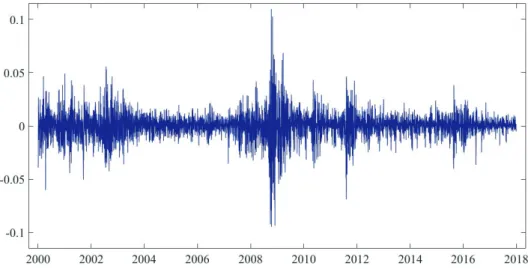
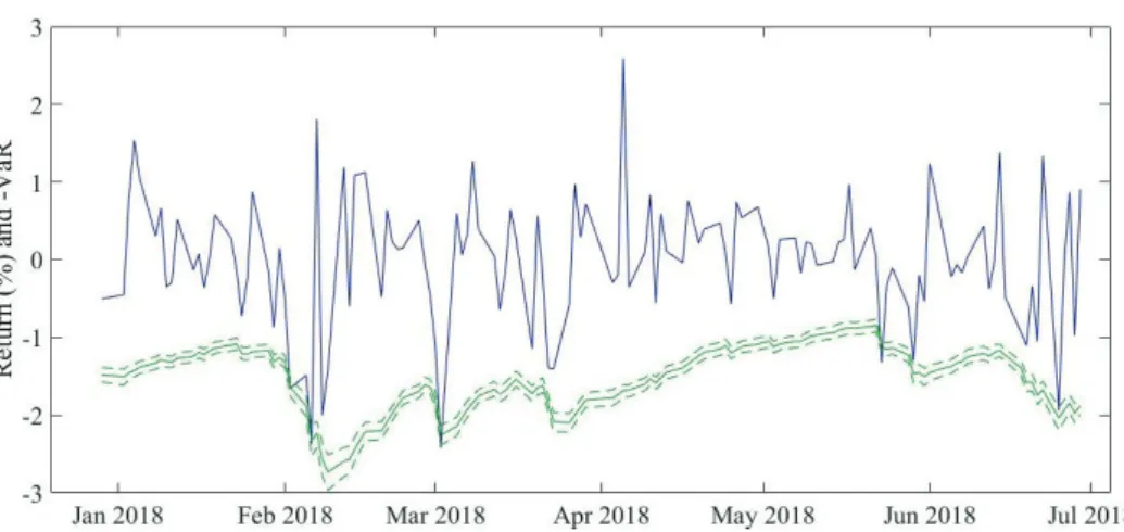
Up to this point, we presumed the data to be i.i.d. and left the time dimension aside. However, most financial data possess a temporal ordering, which frequently reveals unique features of the data. Figure 1.1 plots the log-returns of the S&P500

Figure 1.1: Daily Log-return of the S&P500 index for the years 2000 until 2017.

index for the years 2000 until 2017. We observe that “large changes tend to be followed by large changes, of either sign, and small changes tend to be followed by small changes” (Mandelbrot, 1963), which is known as volatility clustering. To reflect such temporal dependence, we introduce the conditional probability given the pastPt−1[·] =P[·|Xt−1, Xt−2,· · · ·] and denote the conditional mean and

conditional variance associated with _Pt−1 by Et−1 and Vart−1, respectively. In

correspondence to the unconditional volatility measureσ, its conditional counter-partσt= Vart−1[Xt]

1

2 _{depends on X}

t−1,Xt−2, . . . and is therefore a stochastic

process. Similarly, one obtains conditional analogues for VaR and ES.

Definition 1.4. (Conditional Value-at-Risk) Given a levelα∈(0,1), the condi-tionalαVaR is defined byV aRt,α(Xt) =−inf{x∈R:Pt−1[Xt≤x]≥α}.

Definition 1.5. (Conditional Expected Shortfall) Given a level α ∈ (0,1), the conditionalαES is defined byESt,α(Xt) =Et−1[Xt|Xt< V aRα,t].

Again, these risk measures are unobserved by the researcher and must be in-ferred from the data. For this purpose, the stochastic process of the risk measure

is typically parameterized, e.g. σt=σ(Xt−1, Xt−2, . . .;θ), and an estimate of the

risk measure is obtained by replacing the unknown parameters by estimates.

1.4

Contribution and Outline of the Thesis

Several bootstrap methods have been proposed in the literature to quantify the uncertainty around the risk measures’ point estimates. Whereas existing work shows that simulation results are promising, there is, however, no theoretical result underpinning the validity of these methods.

The aim of this thesis is to fill this gap. In particular, we can identify three principal contributions of this thesis. First, we provide a novel, and realistic, justification for commonly constructed intervals around point estimates of condi-tional objects such as condicondi-tional risk measures. This asymptotic justification is of rather theoretical nature and established for a general class of time series models. Second, we propose bootstrap methods to mimic the finite sample distribution of the quasi-maximum-likelihood estimator associated with the conditional VaR and ES. In addition, we give formal proofs of bootstrap consistency, which confirm the validity of those methods. Third, we conduct simulation studies to evaluate the performance of the bootstrap methods in finite samples. Several interval types are investigated and recommendations are made regarding the choice of the interval, which serves as practical guideline for practitioners.

Two challenges arise throughout this thesis. The first issue possesses a funda-mental character and stems from the fact that on one hand one must condition

on the sample as the past informs about the present, yet on the other hand one must allow the data up to now to be treated asrandom to account for estimation uncertainty. The second issue originates from the stochastic nature of the condi-tional risk measures. Because the latter vary over time and they do not permit a limiting distribution, which further complicates the analysis.

Both challenges are addressed in Chapter 2 in detail. Typically, researchers resort to the unrealistic assumption of two-independent processes to bypass the fundamental issue described above. To avoid this assumption, a solution based on a simple sample-split approach is proposed in this chapter, which requires a much more realistic weak dependence condition instead. Further, to acknowledge that the conditional quantities vary over time, a merging concept is employed, which generalizes the notion of weak convergence.

1.4 Contribution and Outline of the Thesis

Chapter 3 verifies the high-level assumptions of the previous chapter for various time series models including autoregressive moving-average (ARMA) and general-ized autoregressive conditional heteroskedasticity (GARCH) type models.

In Chapter 4 we propose a fixed-design residual bootstrap method for the two-step estimator of Francq and Zako¨ıan (2015) associated with the conditional VaR. The bootstrap’s consistency is proven under mild assumptions and boot-strap intervals are constructed for the conditional VaR. A large-scale simulation study supports the theoretical results and sheds further light on the bootstrap’s performance in finite samples.

Chapter 5 builds on the results of Chapter 4. In this chapter a fixed-design residual bootstrap is investigated for the estimator of the conditional ES. The asymptotic validity of the bootstrap scheme is established and a Monte Carlo experiment is carried out to study the finite sample behavior. Simulations confirm that the method performs adequately in samples of modest size.

Chapter 6 provides a short conclusion of the thesis. Proofs of the theoretical results are collected in appendices at the end of each chapter. Whereas notation is consistent within each chapter, it may differ across chapters. Therefore relevant notation is specified within the chapters.

Chapter 2

A Justification of

Conditional Confidence

Intervals

To quantify uncertainty around point estimates of conditional objects such as con-ditional means or variances, parameter uncertainty has to be taken into account. Attempts to incorporate parameter uncertainty are typically based on the unre-alistic assumption of observing two independent processes, where one is used for parameter estimation, and the other for conditioning upon. Such unrealistic foun-dation raises the question whether these intervals are theoretically justified in a realistic setting. This chapter presents an asymptotic justification for this type of intervals that does not require such an unrealistic assumption, but relies on a sample-split approach instead. By showing that our sample-split intervals coin-cide asymptotically with the standard intervals, we provide a novel, and realistic, justification for confidence intervals of conditional objects. The analysis is carried out for a rich class of time series models.1

2.1

Introduction

One of the open questions in time series is how to quantify uncertainty around point estimates of conditional objects such as conditional means or conditional variances. A fundamental issue arises in the construction of confidence intervals that ought to capture the parameter estimation uncertainty contained in these objects. This fundamental issue stems from the fact that on one hand one must

condition on the sample as the past informs about the present, yet on the other hand one must allow the data up to now to be treated asrandom to account for estimation uncertainty. The issue is well-recognized in the econometric literature, however in practice confidence intervals are commonly constructed by treating the sample simultaneously as fixed and random. Frequently, such approach is moti-vated by presuming to have two independent processes. Assuming two independent processes with the same stochastic structure, using one for conditioning and one for the estimation of the parameters, bypasses the issue. It is a mathematically convenient assumption as in such case the uncertainty quantification reduces to an ordinary inferential problem. However, practitioners rarely have a replicate, independent of the original series, at hand with the exception of perhaps some experimental settings. As such, the intervals commonly constructed by practi-tioners lack a satisfactory theoretical justification. Therefore it is the objective of the present work to develop a realistic justification for such confidence intervals around point estimates of conditional objects.

In the literature the fundamental issue described above is encountered in var-ious ways. In the specific case of a first-order autoregressive (AR) process with Gaussian innovations, Phillips (1979) investigates the statistical dependence be-tween the ordinary least squares (OLS) estimator and the endogenous variable conditioned upon. He obtains an Edgeworth-type expansion for the distribu-tion of the condidistribu-tional mean and, further, studies forecasting, where the fun-damental issue equally arises.2 _{L¨utkepohl (2005, p. 95) explicitly states a}

two-independent-processes assumption in connection with vector AR models. He pos-tulates that such assumption is asymptotically equivalent to using only data not conditioned upon for estimation. Ing and Wei (2003) clearly distinguish between

independent-realizationandsame-realizationsettings and study the unconditional mean-squared prediction error in the latter for an infinite-order AR process. In a companion paper they also provide a theoretical verification for order selection

2.1 Introduction

criteria for same-realization predictions and stress that it can be misleading to assume that the results for independent-realization settings carry over to those for corresponding same-realization cases (Ing and Wei, 2005). Other studies inves-tigate parameter uncertainty by using resampling methods, that typically mimic a distribution in which the sample, or at least a subsample, is treated as fixed and random at the same time (cf. Pascual, Romo, and Ruiz, 2004, 2006, Pan and Politis, 2016a, 2016b). Aware of this paradox, Kreiss (2016) points out that condi-tioning on observing specificin-samplevalues affects the parameter estimator, but the effect is often erroneously disregarded. Deviating from the various bootstrap approaches, Hansen (2006) examines parameter uncertainty in interval forecasts in a classical statistical framework. Similar to a general regression framework, he conditions on an arbitrary fixedout-of-sample value to avoid the issue. However, conditioning on arbitrary fixed out-of-sample values appears incompatible with the usual setup of dynamics in which we condition on the final value(s) of the sample. Acknowledging the issue while avoiding the two-independent-processes argument bears careful statements as in Francq and Zako¨ıan (2015) who write in view of this issue “the delta method ... suggests” (p. 162). Similarly, Pesaran (2015) notices that although such intervals “have been discussed in the econometrics literature, the particular assumptions that underlie them are not fully recognized” (p. 389).

This chapter provides a novel, and realistic, justification for commonly con-structed confidence intervals around point estimates of conditional objects. Our solution is based on a simple sample-split approach and a weak dependence con-dition, which allows to partition our sample into two asymptotically independent subsamples. For a rich class of time series models we construct asymptotically valid sample-split intervals, without relying on the assumption of observing two independent processes, and show that these intervals coincide asymptotically with the intervals commonly constructed by practitioners. As will be argued below, an appropriate concept to study conditional confidence intervals is merging, a con-cept that generalizes weak convergence. To the best of our knowledge, excon-cept for Belyaev and Sj¨ostedt-De Luna (2000), the present work is the only one to study merging in the context of conditional distributions. Moreover, we seem to be the first to employ merging of conditional distributions in time series. By employing this concept we avoid unnatural assumptions such as observing Xn =x (in

dy-namic models), losing the time index n, and instead explicitly acknowledge that the conditional objects vary over time.

The rest of this chapter is organized as follows. Section 2.2 specifies the gen-eral setup and describes the argument of two independent processes as well as our sample-split approach. In Section 2.3 we establish merging among the pro-posed and the two-independent-processes estimator in probability under mild con-ditions. Further, we construct asymptotically valid sample-split intervals and show that these coincide asymptotically with the standard intervals. The extension to prediction is discussed in Section 2.4. Section 2.5 concludes. The main proofs are collected in Appendix 2.A, while Appendix 2.B provides additional proofs of intermediate results.

2.2

General Setup

2.2.1

The General Prediction Function

Let {Xt} be a real-valued stochastic process defined on the probability space

(Ω,F,_P). θ denotes a generic parameter vector of length r∈ Nand θ0 the true

value, unknown to the researcher.3 Let Θ⊆Rr be the corresponding parameter

space.

Our general setup involves inference on an object that we call the prediction function, which is a function of both the process{Xt} and of the parameterθ. It

represents the random object of interest, and will typically express quantities such as a conditional mean or conditional variance (without conditioning on a specific value) as a function of the sample.

Definition 2.1. Theprediction function ψ:_R∞×Θ→_Ris depending both on the parameterθand the entire history of the process{Xt}, such that we can write

the prediction of the quantity at timen+ 1, using data up to timen, as

ψn+1:=ψ(Xn, Xn−1, . . .;θ). (2.1)

With this setup we can describe most of the possible applications of interest. We now provide three examples to illustrate the prediction function.

3_{Generally, in particular throughout Section 2.2, we do not distinguish betweenθandθ} 0 if

2.2 General Setup

Example 2.1. Suppose the time series {Xt}follows an AR(1) process given by

Xt=βXt−1+εt, (2.2)

where |β| < 1 and{εt} are independent and identically distributed (i.i.d.) with

E[εt] = 0. The conditional mean ofXn+1 givenXn is

µn+1:=E[Xn+1|Xn] =βXn. (2.3)

Using the prediction function we can then write µn+1 = ψ(Xn, Xn−1, . . .;θ) =

βXn withθ=β.

A more precarious example, due to its large popularity, is the conditional variance in a generalized autoregressive conditional heteroskedasticity (GARCH) model (Engle, 1982; Bollerslev, 1986). Whereas in the previous AR(1) case it suf-fices to condition on the terminal observation, the subsequent Example 2.2 is more extreme as the entire sample contains information about the object of interest.

Example 2.2. Let{Xt} follow a GARCH(1,1) process given byXt=σtεtwith

σ2_t =ω+αX_t2₋₁+βσ2_t−1, (2.4)

where ω >0, α≥0, 1> β ≥0 and {εt} are i.i.d. withE[εt] = 0 andE[ε2t] = 1.

The model’s recursive structure implies

σn2+1= ω 1−β +α ∞ X k=0 βkXn2−k. (2.5)

It follows directly from (2.5) that

σ2_n+1=ψ(Xn, Xn−1, . . .;θ) = ω 1−β +α ∞ X k=0 βkX_n2_−k, withθ= (ω, α, β)0, and Θ⊂(0,∞)×[0,∞)×[0,1).

The next example shows that for a large class of models the prediction function can be written in the form of Definition 2.1.

chain of the form

St=ϕ(St−1, Xt;θ), t= 1,2, . . . (2.6)

where ϕ is some map ϕ : _Ra _×

R×Θ→ Ra. Whereas Xt is observable by the

researcher at time t, St may be unobservable or only partially observable. The

object of interestψn+1is typically a function of the state of the Markov chainSn,

such that ψn+1 =π(Sn;θ) for some functionπ. Through the recursion in (2.6),

this is in turn a function of the past ofXn, such that we may write

ψn+1=π(Sn;θ) =ψn+1(Xn, Xn−1, . . .;θ).

Many stochastic processes are in fact Markov processes, including ARMA and GARCH models, several GARCH extensions such as Zako¨ıan’s (1994) threshold GARCH, and the set ofobservation driven models considered by Blasques, Koop-man, Lasak, and Lucas (2016).

Note that in many cases, such as the GARCH(1,1) of Example 2.2, the pre-diction function actually depends on the infinite past of the series. In order to express (an approximation of) the prediction function in terms of observable vari-ables only, we would need to replaceXtbystfor allt <1, where{st}is a sequence

of (arbitrary) constants to which we refer as starting or initial values. For a fixed n, we accordingly define an approximate prediction functionψs

n+1 :Rn×Θ→R

that is only a function of observable variables and the parameter as

ψs_n+1(X1:n;θ) :=ψ(Xn, Xn−1, . . . , X1, s0, s−1, . . .;θ), (2.7)

where X1:n = (X1, . . . , Xn)0. Note that, given the varying input of the left-hand

side in (3.2), we now actually have a sequence of (varying) functions forn∈N.

In many cases the values far in the past are negligible for a wide range of values for{st}. Consequently,ψns+1will be close toψn+1. This property can be shown to

hold for many different processes including the ones in the examples. We formalize the exact condition we need regarding the negligibility of the starting values in Assumption 2.1.(ii).

Although the prediction function typically represents a conditional object, we have not conditioned on anything yet in the definition. We therefore now extend the analysis by formally conditioning on observing a particular sample. Letx1:n=

2.2 General Setup

(x1, . . . , xn)0 denote a specific sample path of X1:n. Throughout the chapter, we

will discriminate between random variables and their realized counterparts by writing the former in capital and the latter in lowercase letters to avoid ambiguity.

As we will consider sample splitting later on, we define notation that also allows for conditioning on only a subsample. For that purpose, let t1 :t2 denote

the (sub-)period from t1 up to t2, and correspondingly Xt1:t2 = (Xt1, . . . , Xt2)

0

for any integers 1≤t1≤t2≤n, with a corresponding definition for the observed

subsamplext1:t2. Furthermore, letX

c

t1:n= (c1, . . . , ct1−1, Xt1, . . . , Xn)

0_{denote the}

vector where all non-considered subsamples are replaced by a sequence of constants

{ct}, in a similar way as we did for the starting values. We can now formally define

the conditional prediction function.

Definition 2.2. Theprediction function conditional on observing Xt1:n = xt1:n is defined as ψn+1|t1:n:=ψ s n+1(x c t1:n;θ). (2.8)

Note that we phrase the conditional prediction function directly in terms of the approximate prediction functionψns+1rather than the true prediction function. We

take this “shortcut” because we cannot observex0, x−1, . . ., so we cannot condition

on those values anyway. Therefore, the “true” conditional object (which we might represent as ψn+1|−∞:n), is, from an applied point of view, only the theoretical

benchmark.

Example 2.1. (continued) For the conditional mean of an AR(1) process, condi-tioning only on the terminal observationXn=xn suffices; that is, for anyt1≥1

and any sequence{ct}, we have that

ψn+1|t1:n =ψ s n+1(x c t1:n;θ) =βxn=ψ s n+1(x c n:n;θ) =ψn+1|n. (2.9)

Example 2.2. (continued) For objects such as the conditional variance for the GARCH(1,1), the conditioning set and the sequence{ct}make a difference, as

ψn+1|t1:n=ψ s n+1(x c t1:n;θ) = ω 1−β +α n−t1 X k=0 βkx2_n−k +αβn−t1 t1−1 X k=1 βkc2_t 1−k+αβ n ∞ X k=0 βks2_−k, (2.10)

an appropriate choice of t1, our Assumption 2.1.(ii) on the negligibility of the

initial condition, also implies that the difference between ψn+1|t1:n and ψn+1|1:n becomes negligible asymptotically.

Before introducing estimators for θ let us discuss the objects we want to con-struct inference for. In principle there are two unknown objects one could develop statistical intervals for: ψ_ns₊₁(X1:n;θ) (or slightly more generallyψsn+1(X

c t1:n;θ)) andψs

n+1(xct1:n;θ).For a GARCH(1,1), for instance, the first would read as

ψ_ns₊₁(X1:n;θ) = ω 1−β +α n−1 X k=0 βkX_n2_−k+αβn ∞ X k=0 βks2_−k

whereas the second witht1= 1 reads as

ψ_ns₊₁(x1:n;θ) = ω 1−β +α n−1 X k=0 βkx2_n−k+αβn ∞ X k=0 βks2_−k

or more generally, ift1 is not taken to be equal to one, as in (2.10). While

sta-tistical intervals for both objects can be constructed we focus here on conditional inference, i.e. on intervals forψn+1|t1:n =ψ

s

n+1(xct1:n;θ). In a time series context intervals for ψn+1|t1:n are motivated by the relevance property of Kabaila (1999) which postulates that intervals should relate to what actually happened during the sample period opposed to what might have happened. Indeed, intervals for ψn+1|t1:n can theoretically be shown to be considerably shorter than the intervals for their unconditional counterparts. While the unconditional objects might lead to a conceptually easier analysis, our focus on the conditional objects is not only theoretically but also empirically relevant.

Estimating the Prediction Function

As θ is unobserved, we need to estimate it. We assume that the estimator is based on a subsample 1 : nE (with 1 ≤ nE ≤ n) of the process {XtE} which

is potentially adifferent sample than{Xt}that arises in the prediction function.

The estimator ofθbased onXE_1:nE = (X₁E, . . . , X_nE_E)0 will be denoted by ˆθ(XE_1:nE). The introduction of {XE

t } serves three purposes: first, using a different process

allows us to formulate the two-independent-processes argument where XtE =Yt,

with{Yt}independent of{Xt},nE=nand an interval is constructed forψn+1|1:n.

Second, it will allow us to discuss the standard approach whereXE

2.2 General Setup

and an interval is constructed for ψn+1|1:n. Please note already here that this

means that the same variables that arise in the prediction function are also used for estimatingθ. Third, it allows us to define the sample splitting approach which we study here. In this approach XE

t = Xt and an interval is constructed for

ψn+1|nP:n withnE< nP (with 1< nP ≤n) such that in contrast to the standard

approach different subsamples are used for prediction and estimation.

Before we illustrate why the standard approach is problematic for constructing and evaluating conditional intervals, we need to define the final building block of prediction function estimation: the conditional prediction function estimator.

Definition 2.3. Let 1≤nP ≤n. Define theprediction function estimator

condi-tional on observing XnP:n=xnP:n as ψ V n+1|nP:n:=ψ V n+1(xcnP:n,X E 1:nE) =ψ s n+1(xcnP:n, ˆ θ(XE1:nE)). (2.11)

Note that in the above definition we do not condition on the sampleXE

1:nE =

xE1:nEthat is used to estimateθ. The reason for not conditioning onX

E

1:nE =x

E

1:nE

is that the goal is to preserve the randomness in the second argument of ψs n+1,

i.e. in ˆθ(XE

1:nE), and consequently in ψ

V

n+1|nP:n. Hence, if this goal is achieved

we can use the (non-degenerate) conditional (on XnP:n = xnP:n) distribution

of ψ V

n+1|nP:n to construct confidence intervals for ψn+1|nP:n. Having this said

let us have a closer look at the standard approach. As mentioned above in the standard approach one has XE

t = Xt, nP = 1 and nE = n. Hence, denoting

by ψ VST A

n+1|1:n the “standard” estimator of the prediction function conditional on

observingX1:n =x1:n, it becomes ψ VST A n+1|1:n :=ψ V n+1(x1:n,x1:n) =ψns+1(x1:n,θˆ(x1:n)). (2.12)

Notice that there is no capitalXin (2.12) because there is only one sample and one typically conditions on all values of this sample. Hence, (2.12) is non-random and thus does not have a distribution that could be used to construct intervals. Instead, to still be able to construct a “standard-looking” interval in practice, researchers typically implicitly rely on the (approximate) quantiles of the estimator

ψ VST A∗

n+1|1:n :=ψ

V

n+1(x1:n,X1:n) =ψns+1(x1:n; ˆθ(X1:n)). (2.13)

It is well understood in the literature that considering the sample as random and non-random at the same time as in (2.13) does not provide a fully satisfactory

justification of the intervals used in practice. For the readers not so familiar with the problem just discussed we provide two examples that both illustrate the problem arising from (2.13). The examples illustrate that the severity of the problem may vary; ranging from only complicating the analysis (Example 2.1) to making the analysis impossible (Example 2.2).

Example 2.1. (continued) For the AR(1), we know from (2.9) thatψn+1|1:n =

ψs

n+1(x1:n, θ) =βxn. Estimatingβ by OLS, say ˆβ(X1:n), the estimator in (2.13)

becomes

ψ VST A∗

n+1|1:n =ψn+1(x1:n; ˆθ(X1:n)) =ψns+1(x1:n,βˆ(X1:n)) = ˆβ(X1:n)xn. (2.14)

Note the discrepancy in treating the terminal observation as random in the esti-mation sample, yet fixed for the prediction sample. To construct an interval for βxn, one uses

√

n βˆ(X1:n)−β

d

→N(0, σβ2) (2.15)

with σ_β2 = 1−β2 (cf. Hamilton, 1994, p. 215) and that one can estimate the variance of this normal distribution by ˆσ2

β(X1:n) = 1−βˆ(X1:n)2. Then an interval

forβxn is typically constructed the following way:

ˆ

β(X1:n)xn±Φ−1(γ/2)xnˆσβ(X1:n)/

√

n, (2.16)

where Φ−1denotes the standard normal quantile function. However, the interval in (2.16) is hard to interpret as the terminal observation is treated simultaneously as fixed and random. In essence, researchers typically approximate the distribution of

√

n( ˆβ(X1:n)−β)xn instead of the conditional distribution of

√

n( ˆβ(X1:n)−β)Xn

given Xn = xn. The approximation of the latter appears rather cumbersome

because even the rather simple condition Xn =xn has an influence on the whole

series X1:n (Kreiss, 2016). Despite the challenge, Phillips (1979) obtains such

approximation based on Edgeworth expansions in the case ofεt iid

∼ N 0, σ2ε

.

Example 2.2. (continued) For the conditional variance of the GARCH(1,1), the standard estimator of the prediction function conditional onX1:n=x1:n, is given

2.2 General Setup by ˆ σ_n2₊₁ST A_|1:n=ψs_n+1 x1:n; ˆθ(x1:n) = ωˆ(x1:n) 1−βˆ(x1:n) + ˆα(x1:n) n−1 X k=0 ˆ β(x1:n)kx2n−k + ˆα(x1:n) ˆβ(x1:n)n ∞ X k=0 ˆ β(x1:n)ks2−k, (2.17) where ˆθ(x1:n) = ωˆ(x1:n),αˆ(x1:n),βˆ(x1:n) 0

is some estimate for θ depending on x1:n. Clearly, (2.17) illustrates for the GARCH(1,1) the above mentioned

prob-lem that the standard estimator is not random (after conditioning). For the GARCH(1,1) the estimator in (2.13) whose quantiles are used for an interval reads as ˆ σ2n+1ST A∗=ψn+1 x1:n; ˆθ(X1:n) = ωˆ(X1:n) 1−βˆ(X1:n) + ˆα(X1:n) n−1 X k=0 ˆ β(X1:n)kx2n−k + ˆα(X1:n) ˆβ(X1:n)n ∞ X k=0 ˆ β(X1:n)ks2−k. (2.18)

This quantity exemplifies for the GARCH(1,1) that the complete sample is re-garded as random and non-random at the same time. While for the AR(1) this complicated the analysis, yet not made it impossible, the dependence on the com-plete sample here makes it difficult to use this quantity to make meaningful prob-abilistic statements.

2.2.2

Argument of Two Independent Processes

The argument of two independent processes can at least be traced back to Akaike (1969), who studies the prediction of AR time series. It reoccurs in Lewis and Reinsel (1985, p. 394): “...the series used for estimation of parameters and the series used for prediction are generated from two independent processes which have the same stochastic structure.” The same argument also appears in L¨ utke-pohl (2005, p. 95) and in Dufour and Taamouti (2010). Let {Yt} be a process

independent of {Xt} defined on the same probability space (Ω,F,P) with {Yt}

the process{Xt}, suppose there is a sample Y1:n := (Y1, . . . , Yn)0 of the process

{Yt} that we use as estimation sample, that is XE1:n =Y1:n. In this situation we

denote the conditional prediction function estimator of Definition 2.3 byψ V2IP n+1|1:n and it equals ψ V2IP n+1|1:n :=ψ V n+1(x1:n,Y1:n) =ψns+1(x1:n; ˆθ(Y1:n)). (2.19)

Notice that (2.19) does not have the same shortcoming as (2.13) because even if we considerx1:n to be known we can nevertheless consider ˆθ(Y1:n) to be random

and can hence use its distribution to construct intervals. Throughout this chapter, we call (2.19), the 2IP (two independent processes) estimator. Then, a conditional intervalI2IP

γ (x1:n,Y1:n) can be based on the (approximate) quantiles ofψ

V2IP n+1|1:n. It satisfies P h I_γ2IP(x1:n,Y1:n)3ψn+1|1:n X1:n =x1:n i = (≈)1−γ, (2.20)

with the approximate sign indicating asymptotic equivalence. Note that the in-dependence implies that the distribution of Y1:n in (2.20) does not depend on

the realizationx1:n, yet the statement does depend on x1:n because the interval

depends on it (for the AR(1) this can be directly seen from (2.16) when replacing X1:nbyY1:n). Although the 2IP approach is statistically sound, it assumes two

in-dependent processes with the same stochastic structure. Phillips (1979) points out that the assumption “is quite unrealistic in practical situations” (p. 241). Indeed, it is difficult to imagine this assumption to be satisfied in any real-life applica-tion beyond experimental settings. Moreover, as only one sample realizaapplica-tion is available, to compute the estimate of the intervalIγ2IP(x1:n,Y1:n) it is frequently

suggested to takeY1:n =x1:n, violating the independence assumption. Thus, the

2IP approach appears to be a rather questionable justification for the usual inter-val, and as such, in this work we provide an alternative, realistic, justification of (asymptotically equivalent) intervals based on sample splitting.

2.2.3

Sample-split Estimation

An intuitive motivation for the sample-split approach is the successive decline of the influence of past observations present in a substantial class of time series models. This property permits to split our sample into two (asymptotically) inde-pendent subsamples. Consider the end point of the estimation sample,nE, and the

2.2 General Setup

starting point of the prediction sample,nP satisfying 1< nE < nP ≤n, such that

the two samples are non-overlapping. In this situation we denote the conditional prediction function estimator of Definition 2.3 byψ

VSP L n+1|nP:n and it is given by ψ VSP L n+1|nP:n:=ψ V n+1(x c nP:n,X1:nE) =ψ s n+1(x c nP:n; ˆθ(X1:nE)). (2.21)

Throughout the chapter, we call (2.21) the SPL estimator (due to splitting). Sim-ilar to the two sample approach, we can consider the first argument of ψsn+1 in

(2.21) as given and the second argument as random since the subsamples are non-overlapping. A conditional intervalISP L

γ (xnP:n,X1:nE) can be constructed such

that P h I_γSP L(xnP:n,X1:nE)3ψn+1|nP:n XnP:n=xnP:n i = (≈)1−γ. (2.22)

This statement does make sense as there is still randomness in ˆθ(X1:nE) since

X1:nE is not conditioned upon, yet the last n−nP + 1 values of {Xt}

n t=1 are

fixed such that their randomness is not taken into account. Similar to (2.20), the statement in (2.22) does depend on xnP:n and in contrast to x1:n in (2.20) the

realization xnP:n may influence the distribution of X1:nE. However, as said at

the beginning of this subsection the idea of the sample-split approach is that this dependence will vanish asymptotically.

Remark 2.1. In Section 2.3 we will discuss hownE andnP should be chosen from

an asymptotic perspective to ensure that our regularity conditions are fulfilled. As we only consider sample splitting as a theoretical approach to validate commonly constructed conditional confidence intervals, these asymptotic guidelines are suf-ficient for our purposes and we do not have to consider how to choose nE and

nP in practice. Of course, one could use the sample-split approach in practice to

construct confidence intervals. While one would gain (near) independence between the two subsamples, this would come at a cost of less estimation precision as fewer observations are used for parameter estimation. For the Gaussian AR(1) setting, Phillips (1979) derives asymptotic expansions for the case where, in our notation, nE=n−landnP =nfor somel≥0, showing that even in this simple case there

is indeed a trade-off as described above and the optimal choice oflis unclear. An interesting extension of our analysis would therefore be to investigate the optimal choices of nE and nP to achieve the most accurate confidence intervals in small

model and as such would have to be investigated on a case-by-case basis. This is therefore outside the scope of the current work.

2.3

Asymptotic Justification

In this section, we connect the sample-split procedure of Section 2.2.3 with the two-independent-samples approach of Section 2.2.2. First, in Section 2.3.1, we show that the notion of weak convergence is inadequate to study asymptotic closeness for objects that vary over time and discuss the concept of merging. Then, in Sec-tion 2.3.2 we link the 2IP and the SPL estimator by proving that their condiSec-tional distributions merge in probability (Theorem 2.1). Thereafter, in Section 2.3.3, we construct asymptotically valid intervals (Theorem 2.2) and show that the sample-split intervals coincide asymptotically with the intervals commonly constructed by practitioners (Theorem 2.3). Last, in Section 2.3.4, we state intervals of re-duced form and simplified theoretical results under asymptotic normality of the parameter estimator.

2.3.1

Merging

To illustrate the inappropriateness of weak convergence in the context considered here, we revisit Example 2.1 for the 2IP approach and the SPL approach, which shows that studying asymptotic closeness between conditional distributions is often complicated by the absence of a limiting distribution.

Example 2.1. (continued) For the 2IP approach (2.15) implies that√n βˆ(Y1:n)−

β d

→N(0, σ2

β) and it entails that

√

n( ˆβ(Y1:n)−β)xconverges weakly toN(0, σβ2x2)

for any fixed x 6= 0. Further, the result suggests that the conditional distribu-tion of √n( ˆβ(Y1:n)−β)Xn given Xn = xn, which is just the distribution of

√

n( ˆβ(Y1:n)−β)xn, is asymptotically close toN(0, σβ2x

2

n). Similarly, for the

SPL-approach withnE/n→1 we have

√

n βˆ(X1:nE)−β

d

→N(0, σ2

β) which suggests as

well (if the gap betweennEandnis large enough which will be formally specified

below) that the conditional distribution of√nE( ˆβ(X1:nE)−β)Xn givenXn=xn

is also close to N(0, σ2

βx

2

n). For both approaches the approximating distribution

N(0, σ2

βx2n) varies withnthrough the terminal realizationxn. Note that the

2.3 Asymptotic Justification

asymptotic closeness, as it requires a (fixed) limiting distribution, which is absent here.

Next, we discuss what closeness means in the absence of a limiting distribution. To do so, first recall that weak convergence of a sequence of cdfs {Fn} on Rk

with k∈_N, i.e.Fn(τ)→F(τ) for all continuity points τ ofF, can alternatively

be defined by dBL(Fn, F)→0. Here dBL denotes the bounded Lipschitz metric

defined by dBL(F, G) = sup Z f d(F−G) :||f||BL≤1 , (2.23)

where for any real-valued function f on Rk one puts ||f||BL = supx

f(x)

+

sup_x6=y |f(_||x_x)−₋f_y||(y)|, with|| · ||denoting the Euclidean norm, i.e. ||A||=ptr(A0_A)

for any vector or matrixA. Following Dudley (2002) (see D’Aristotile, Diaconis, and Freedman (1988) and Davydov and Rotar (2009) for related work) we state the following definition.

Definition 2.4. (Merging) Two sequences of cdfs {Fn} and {Gn} are said to

merge if and only if dBL(Fn, Gn)→0 asn→ ∞.

Note that weak convergence can be seen as a special case of merging with Gn = Gfor all n ∈N. While merging is appropriate to capture the asymptotic

closeness of the conditional distribution of√n( ˆβ(Y1:n)−β)Xn andN(0, σ2βx2n) for

a given sampleXn =xn, we now extend the concept in a way that allows us to

deal with asymptotic closeness when we do not condition on a particular sample. The necessity of this definition can again be exemplified by the AR(1), which also illustrates how we will deal with the dependence of the statements in (2.20) and in (2.22) on the sample that we mentioned below these equations. For instance, in Example 2.1 as described at the beginning of this section, the goal would be to formalize a statement like ‘whennis large, the probability of allxn such that the

distribution of√n( ˆβ(X1:n)−β)xn merges with that of

√

nE( ˆβ(X1:nE)−β)xn is

approximately equal to one’. We now first introduce the conditional distributions of the 2IP and the SPL estimator in the general case and then give the definition capturing what we just illustrated for the AR(1).

Let mn be a sequence of normalizing constants with mn → ∞ (e.g. mn =

√ n). For anyt1≥1, we define the subσ-algebraIt1:n=σ(Xt:t1≤t≤n). We denote

theconditional cdfs of the 2IP and SPL estimator by F_n2IP(τ|I1:n) :=Pmn ψ V n+1(X1:n,Y1:n)−ψn+1 ≤τI1:n (2.24) F_nSP L(τ|InP:n) :=P mn ψ V n+1(XnP:n,X1:nE)−ψn+1 ≤τInP:n , (2.25)

respectively, so that by specifying an event of I1:n and InP:n, we see that (2.24)

and (2.25) are just the centered and scaled distributions of (2.19) and (2.21), respectively. Please note that (2.25) actually also depends on c, see (2.21), but since our assumptions will ensure that this dependence vanishes asymptotically we prefer to suppress the dependence onchere.

Remark 2.2. Although not explicitly mentioned above we consider (2.24) and (2.25) to be regular conditional cdfs, i.e. we assume that F_n2IP(·|I1:n)(ω) and

FSP L

n (·|Inp:n)(ω) are cdfs for everyω ∈Ω; for the exact definition and the

exis-tence see Dudley (2002, Section 10.2).

We can now define merging in probability (we do so without explicitly using the conditional cdfs of the 2IP and the SPL approach).

Definition 2.5. (Merging in probability) Two sequences of conditional cdfs{Fn}

and {Gn} are said to merge in probability if and only if dBL(Fn, Gn) p

→ 0 as n→ ∞, where “→p” denotes “convergence in probability”.

2.3.2

Merging of 2IP and SPL in Probability

Here, we give conditions such that the conditional cdfs of the 2IP and SPL esti-mator merge. Clearly, the conditional confidence intervals are functions of these distributions so that their merging is a building block for the study of the condi-tional confidence intervals based on them. The conditions we give are divided into three parts. Roughly speaking, the first part (general assumptions) makes sure that the function we want to predict is well behaved and that we can estimate the parameter it depends on. The second part (two independent processes) and third part (SPL estimator) guarantee that these assumptions are met by the 2IP and the SPL method. To write the conditions in compact form we employ the usual stochastic order symbols Op and op. We assume thatθ0 belongs to the interior

of Θ, i.e. θ0 ∈ ˚Θ, and we denote the set of all bounded, real-valued Lipschitz

functions onRr byBL=h:Rr→R:||h||BL<∞ . We start with the general

2.3 Asymptotic Justification

Assumption 2.1. (General assumptions)

(i) (Estimator) mn θˆ(X1:n)−θ0

d

→G∞ as n→ ∞ for some cdf G∞ : Rr →

[0,1];

(ii) (Differentiability)ψ(·;θ) is continuous on Θ and twice differentiable on ˚Θ; (iii) (Gradient) ∂ψ(Xn,Xn−1,...;θ0) ∂θ =Op(1);

(iv) (Hessian) sup_θ∈V(θ 0) ∂2_ψ(X n,Xn−1,...;θ) ∂θ∂θ0

= Op(1) for some open

neighbor-hood V(θ0) aroundθ0;

(v) (Initial condition) Given sequences{st}and{ct}, we have

mn ψns+1(X c t1:n;θ0)−ψ(Xn, Xn−1, . . .;θ0) =op(1), ∂ψs n+1(Xct1:n;θ0) ∂θ − ∂ψ(Xn, Xn−1, . . .;θ0) ∂θ =op(1), sup θ∈V(θ0) ∂2ψns+1(Xct1:n;θ) ∂θ∂θ0 − ∂2ψ(Xn, Xn−1, . . .;θ) ∂θ∂θ0 =op(1)

for any t1 ≥1 such that (n−t1)/ln → ∞ as n → ∞ and for some

model-specificln withln → ∞.

Assumption 2.1.(i) implies the existence of a limiting distribution for the pa-rameter estimator. The differentiability assumption in 2.1.(ii) plus the bounded-ness Assumptions 2.1.(iii) ensure that the scaled prediction function estimators can accurately be approximated by a Taylor expansion; see Lemma 2.1 for details. Assumption 2.1.(v) with t1 = 1 ensures the negligibility of the starting values

when using the full-sample for prediction, while takingt1 =nP ensures that this

extends to the case where additionallyX1, . . . , XnP−1 are replaced by constants,

i.e. where only the subsample (XnP, . . . , Xn) is used for prediction. This

assump-tion implicitly limits the choice of nP; as replacing past values ofXt fort < nP

by arbitrary constants should have a negligible effect, n−nP needs to increase

faster than some lower boundln. For models exhibiting an exponential decay in

memory, it typically suffices to takeln= logn(see Chapter 3, Equation (3.13)).

For the 2IP estimator, we additionally need the two-independent-processes as-sumption, which is formalized in Assumption 2.2.

(i) (Existence){Yt} is a process defined on (Ω,F,P), distributed as{Xt};

(ii) (Independence){Yt} is independent of{Xt}.

For the SPL estimator we replace the two-independent-processes assumption by a stationarity and a weak dependence condition, which allows to split our sample into two (asymptotically) independent and identical subsamples. In addition we need an assumption onnP andnE as functions ofn, that isnE(n) andnP(n).

Assumption 2.3. (SPL estimator)

(i) (Rates) The functionsnP :N→NandnE :N→NsatisfynE(n)< nP(n)

for alln, while n−nP(n)

ln → ∞andmnE(n)/mn→1 asn→ ∞;

(ii) (Strict stationarity){Xt}is a strictly stationary process;

(iii) (Weak dependence){Xt}satisfies for eachh∈BL

Z h dGSP L_n E (·|InP:n)−G SP L nE _p →0 as n→ ∞, whereGSP LnE (·|InP:n) denotes the conditional cdf ofmnE θˆ(X1:nE)−θ0

given

InP:n andG

SP L

nE the corresponding unconditional cdf.

The subsample size assumption in 2.3.(i) ensures that the number of observa-tions used for conditioning is increasing, which along with the negligibility of the initial conditions implies that the truncation of the prediction function is negligi-ble. Furthermore, the sample size used for estimation should increase fast enough that the respective scaling of the 2IP and SPL estimators, mn andmnE

respec-tively, are asymptotically identical. Ifmn increases no faster than a polynomial

rate, which is generally the case, it is sufficient that nE/n→1 formnE/mn→1

to hold.

The stationarity assumption in 2.3.(ii) can actually be relaxed; what matters is that the conditions in Assumption 2.1 are still true if only a subsample is consid-ered. In particular, we need thatmnE θˆ(X1:nE)−θ0

d

→G∞, which - along with

the assumptions on gradient and Hessian - is certainly satisfied under stationarity. However, in general the assumption will be far too strict; here we use it simply to have a clear, interpretable assumption rather than a list of high-level assumptions that are difficult to interpret. The weak dependence condition in 2.3.(iii) is met

2.3 Asymptotic Justification

by numerous Markov processes. Intuitively, (X1, . . . , XnE) and (XnP, . . . , Xn)

ap-proach independence as their temporal distancenP −nE increases. We illustrate

a particular case in the Remark 2.3.

Remark 2.3. Suppose {Xt} is strong mixing (cf. Doukhan, 1995) and let α

de-note the strong mixing coefficient. For h∈ BL and for all > 0, Markov’s and Ibragimov’s inequality (cf. Hall and Heyde, 1980, Theorem A.5) imply

P Z h dGSP L_n E (·|InP:n)−G SP L nE ≥ ≤1 E Z h dGSP L_nE (·|InP:n)−G SP L nE =1 Cov hmnE θˆ(X1:nE)−θ0 ,signn Z h dGSP L_nE (·|InP:n)−G SP L nE o ≤4||h||BL α(nP−nE).

TakingnP−nE→ ∞such thatα(nP−nE)→0 verifies Assumption 2.3.(iii).

Assumptions 2.1 to 2.3 are met by the AR and GARCH processes considered in Examples 2.1 and 2.2 (with Assumption 2.1.(v) holding for bounded sequences). A detailed verification of each assumption under mild conditions is provided in Chapter 3. We state the following theorem.

Theorem 2.1. (Merging of 2IP and SPL) If Assumptions 2.1 to 2.3 hold, then

Fn2IP(·|I1:n) andFnSP L(·|InP:n)merge in probability.

Having established asymptotic closeness between the conditional cdfsF2IP n (·|I1:n)

andF_nSP L(·|InP:n), we now turn to the construction of asymptotic intervals.

2.3.3

Interval Construction

Henceforth, for any cdf F we write F−1 _{to denote its generalized inverse given}

by F−1_{(u) = inf}

τ ∈ R : F(τ)≥ u . A confidence interval for ψn+1 based on

quantiles of (2.24) or (2.25) is typically infeasible as these cumulative distribution functions are unknown for finiten. Here, they are infeasible because roughly they are the distribution functions of some weights which induce merging multiplied by mn θˆ(X1:n)−θ0

and mnE θˆ(X1:nE)−θ0

, respectively, where, in general, the distributions of mn θˆ(X1:n)−θ0 and mnE θˆ(X1:nE)−θ0

are unknown in finite samples. Since these are the only unknown distributions an asymptotic

approximation can be based onG∞with merging induced by the non-convergent

weights. In general, we also need to estimateG∞; see Examples 2.4 and 2.5 below

for common approaches. We denote estimators of (2.24) and (2.25) resulting from this approximation by F2IP n V (·) and FSP L n V

(·), respectively. In the next subsection we provide explicit expressions whenG∞ is multivariate normal. For the general

construction, we refer to relations (2.42) and (2.43) in Appendix 2.A and the explanations preceding these relations. Based on the 2IP approach, we consider an interval of the form

I_γ2IP(x1:n,Y1:n) = ψ V2IP n+1|1:n− F2IP n V−1 (1−γ2) mn , ψ V2IP n+1|1:n− F2IP n V−1 (γ1) mn , (2.26)

where γ1, γ2 ∈[0,1) satisfyγ =γ1+γ2. We typically takeγ1 =γ2 =γ/2 such

that the interval is equal-tailed. Similarly, we construct the following sample-split interval: I_γSP L(xc_nP:n,X1:nE) = ψ VSP L n+1|nP:n− FSP L n V−1 (1−γ2) mn , ψ VSP L n+1|nP:n− FSP L n V−1 (γ1) mn . (2.27)

To achieve correct coverage, we need thatFn2IP

V

(·) andFn2IP(·|I1:n) merge in

prob-ability and likewise for SPL. A sufficient condition for this in our setting is that we can consistently estimate the asymptotic distribution of the parameter estimator, G∞, by an appropriate estimator. This is formulated in Assumption 2.4 below.

Assumption 2.4. (CDF estimator) LetG V

n(·) denote a random (r-dimensional)

cdf as a function of X1:n, used to estimate G∞: i.e. R h dG V n(·) p → R h dG∞ as n→ ∞for allh∈BL.

Although we did not explicitly specify in Assumption 2.4 the dependence of G V

n

on X1:n, it should be understood to hold for any subsample of X1:n whose size

goes to infinity. The verification of Assumption 2.4 is a standard step in asymp-totic analysis. The two examples below provide common methods for verifying Assumption 2.4.

Example 2.4. Suppose that G∞ belongs to some parametric family {Gθ,ξ|θ ∈

2.3 Asymptotic Justification

some consistent estimators ˆθ(X1:n) and ˆξ(X1:n) for θ0 andξ0 respectively, it

fol-lows from the continuous mapping theorem that G V

n = G_θˆ_(X1:n),ξˆ_(X1:n) satisfies

Assumption 2.4 ifGθ,ξ is continuous in θandξ.

Example 2.5. If ˆGn is based on a consistent bootstrap procedure for G∞ then

Assumption 2.4 clearly holds.

The following theorem states the intervals’ asymptotic validity.

Theorem 2.2. (Asymptotic coverage)

1. (i) Under Assumption 2.1, 2.2 and 2.4, F_n2IP(·|I1:n) and Fn2IP

V

(·) merge in probability.

(ii) If in addition Fn2IP

V

(·)is stochastically uniformly equicontinuous, then P h Iγ2IP(x1:n,Y1:n)3ψn+1 I1:n i _p →1−γ. (2.28)

2. (i) Under Assumption 2.1, 2.3 and 2.4,FSP L

n (·|InP:n)andF SP L n V (·)merge in probability. (ii) If in additionFnSP L V

(·)is stochastically uniformly equicontinuous, then P h I_γSP L(xc_nP:n,X1:nE)3ψn+1 InP:n i _p →1−γ. (2.29) However, the standard approach, motivated byI_γ2IP as in (2.28), computes an interval of the formIST A

γ (x1:n,x1:n) =Iγ2IP(x1:n,x1:n) as only one sample

realiza-tion is available. This, of course, strongly violates the independence assumprealiza-tion of{Xt}and{Yt}. Specifically, replacingY1:n byX1:n in equation (2.26), leads to

I_γST A∗(x1:n,X1:n) = ψ VST A∗ n+1|1:n− FST A n V−1 (1−γ2) mn , ψ VST A∗ n+1|1:n− FST A n V−1 (γ1) mn , (2.30) whereFST A n V

(·) is defined in relation (2.44) and the text preceding it. Whereas it is difficult to justify a conditional confidence interval likeIST A

γ (x1:n,X1:n) directly

due to the lack of randomness, we can provide a justification by characterizing how closely the interval resembles the SPL interval. We establish the asymptotic equivalence, defined in terms of location and (scaled) length, between the two