Drone Obstacle Avoidance and Navigation Using Artificial Intelligence

Degree Programme of Computer Science and Engineering

Niroj Pokhrel

Drone Obstacle Avoidance

and Navigation

using Artificial Intelligence

Master’s Thesis Espoo, April 20, 2018

Supervisor: Professor Alex Jung

Degree Programme of Computer Science and Engineering MASTER’S THESIS Author: Niroj Pokhrel

Title:

Drone Obstacle Avoidance and Navigation using Artificial Intelligence

Date: April 20, 2018 Pages: xii + 102 Professorship: Embedded System Code: SCI3024 Supervisor: Professor Alex Jung

Instructor: Enrique Ramirez M.Sc. (Tech.)

This thesis presents an implementation and integration of a robust obstacle avoid-ance and navigation module with ardupilot. It explores the problems in the cur-rent solution of obstacle avoidance and tries to mitigate it with a new design. With the recent innovation in artificial intelligence, it also explores opportunities to enable and improve the functionalities of obstacle avoidance and navigation using AI techniques. Understanding different types of sensors for both naviga-tion and obstacle avoidance is required for the implementanaviga-tion of the design and a study of the same is presented as a background. A research on an autonomous car is done for better understanding autonomy and learning how it is solving the problem of obstacle avoidance and navigation. The implementation part of the thesis is focused on the design of a robust obstacle avoidance module and is tested with obstacle avoidance sensors such as Garmin lidar and Realsense r200. Image segmentation is used to verify the possibility of using the convolutional neural network for better understanding the nature of obstacles. Similarly, the end to end control with a single camera input using a deep neural network is used for verifying the possibility of using AI for navigation. In the end, a robust obstacle avoidance library is developed and tested both in the simulator and real drone. Image segmentation is implemented, deployed and tested. A possibility of an end to end control is also verified by obtaining a proof of concept.

Keywords: artificial intelligence, drones, obstacle avoidance, autonomous navigation, computer vision, deep neural network, ardupilot Language: English

This thesis is developed in collaboration with Nokia Networks and Depart-ment of Machine Learning for Big Data Group of Aalto University of School of Science. I would like to thank Nokia for providing opportunity and sup-port to undertake this project. I am especially grateful towards my supervisor Professor Alex Jung who incited an interest in Machine learning when I was taking his course on Basics in Machine Learning in Aalto University. His insight and feedback helped in structuring and developing the thesis. The motivation and constant support from my advisor Enrique Ramirez helped me overcome several hurdles.

Espoo, April 20, 2018 Niroj Pokhrel

2.1 Navigation Unit . . . 7

2.2 Optical Flow sensor with CMOS image, gyroscope and ultrasonic[34] 9 2.3 Obstacle Avoidance Unit with corresponding components . . . 12

2.4 Garmin Lite . . . 12

2.5 Velodyne . . . 12

2.6 Rplidar . . . 12

2.7 Intel Realsense R200 [53]. . . 14

2.8 Intel Realsense R200 internals as provided in [53]. . . 14

2.9 Polar Obstacle Density [20] . . . 15

2.10 Vertical Field Histogram [10] showing the formation of polar obstacle densities in front of the vehicle. . . 16

2.11 Aritificial Intelligence Unit showing different components in-volved for developing an intelligent system. . . 17

2.12 Nvidia Jetson TX2 model [52] . . . 20

2.13 Single Neuron[38] . . . 21

2.14 Sigmoid Function . . . 22

2.15 Tanh . . . 23

2.16 ReLU . . . 23

2.17 Multilayer Perceptron [38] . . . 24

2.18 Convolutional Neural Network Internal [38] . . . 25

2.19 Convolutional Neural Network [38] . . . 27

2.20 Training and deploying deep learning with DIGITS [17] . . . 28

2.21 Reinforcement Learning . . . 30

3.1 Autonomous Car architecture [45] . . . 33

3.2 Training End to End FCNN for autonomous driving [9] . . . . 36

3.3 Deploying End to End FCNN for autonomous driving [9] . . . 37

4.1 Four rotors in Quadrotor [58] . . . 39

4.2 Thrust on four rotors [58] . . . 40

4.3 Ascend and Descend [58] . . . 41

4.4 Turning Left and Turning Right [58] . . . 41

4.7 Different Software Components . . . 44

4.8 Apm planner 2 home screen [61] . . . 45

4.9 Apm planner 2 creating mission interfaces [61] . . . 45

4.10 UpBoard [4] . . . 46

4.11 Raspberry Pi [3] . . . 46

4.12 Pixhawk [2] . . . 47

4.13 Mavlink Packets [1] . . . 49

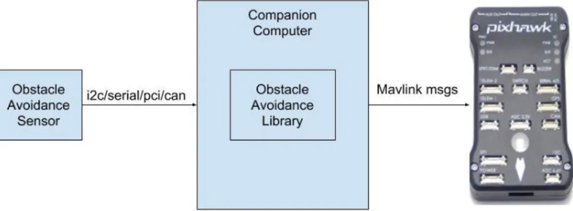
5.1 High Level Architecture of Obstacle Avoidance System . . . . 55

5.2 Main Modules of Obstacle Avoidance Library . . . 55

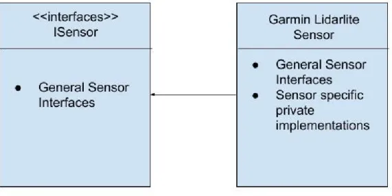
5.3 Sensor Interfaces and Implementation for Garmin lidar lite . . 56

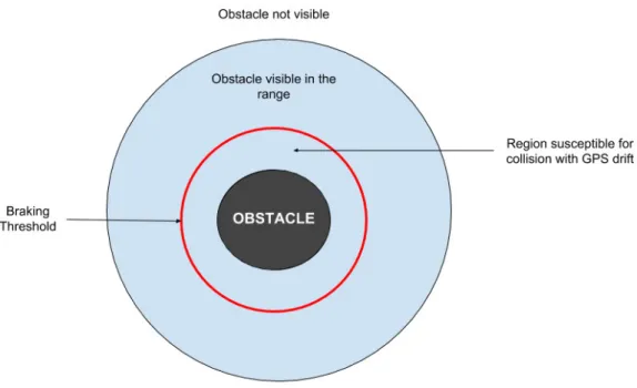
6.1 Different regions of interest around the obstacle . . . 63

6.2 State diagram of sensor fusion algorithm . . . 64

6.3 Simulate obstacle avoidance with Garmin Lidar . . . 64

6.4 Ardupilot sitl with mavproxy for simulating quadrotor drone. . 65

6.5 Integrate obstacle avoidance with Garmin Lidar . . . 66

6.6 Measurement of relative altitude with GPS amidst tall buildings. 67 6.7 Update rate of different sensors. . . 67

6.8 Distance measured with garmin lidar from same distance but different reflective surfaces. . . 68

6.9 Integrate obstacle avoidance with Realsense(r200) . . . 69

6.10 Segmentation of depth image for calculating polar histogram . 71 6.11 Flow chart for calcualating POD and avoiding obstacles . . . . 72

6.12 Simulate obstacle avoidance with Realsense(R200) in gazebo . 73 6.13 POD for obstacles on the right as bright and error on the left 74 6.14 POD for obstacles on the right and left . . . 74

6.15 POD for obstacles on the left and middle . . . 74

6.16 POD for obstacles only in the middle . . . 74

6.17 Noisy data from Realsense camera r200 module. . . 75

6.18 Obstacle Avoidance Architecture with AI . . . 77

6.19 Flow Chart of image segmentation . . . 78

6.20 Fully convolutional neural network for image segmentation [46] 79 6.21 Learning rate in different epochs generated from DIGITS . . . 79

6.22 Training and validation error in different epochs generated from DIGITS . . . 80

6.23 Test input data from [16] . . . 81

6.24 Output from the model for test input data . . . 82

6.25 Image facing Left [30] . . . 84

6.28 Image facing right response in Gazebo . . . 86 6.29 Image facing middle [30] . . . 87 6.30 Image facing middle response in Gazebo . . . 88

4.1 Mavlink Packet Field Description [1] . . . 48 6.1 State Transition Table . . . 62 6.2 Comparison between Garmin lidar and R200 . . . 89

UAV Unmanned Aerial Vehicle AI Artificial Intelligence

ML Machine Learning

GPS Global Positioning System SLAM Self-localizing and Mapping GPU Graphical Processing Units IMU Inertial Measurement Units Lidar Light Detection and Ranging

Radar Radio Detection and Ranging System Sonar Sound navigation and ranging

UHF Ultra-high frequency

ASIC Application Specific Integrated Circuit

NED North East Down

ECEF Earth Centered Earth Fixed VFH Vertical Field Histogram VCP Vehicle Center Point POD Polar Obstacle Density SAD Sum of Absolute Difference ReLU Rectified Linear Unit

CNN Convolutional Neural Network MLP Multi-Layer Perceptron

SVM Support Vector Machine ESC Electronic Speed Controller

RC Radio Controller

PWM Pulse Width Modulation GCS Ground Control Station MAV Micro Aerial Vehicle

PID Proportional Integration Differentiation EKF Extended Kalman Filter

SITL Software In The Loop

RTL Return To Launch

DNN Deep Neural Network

GIS Geographic Information System

RGB Red Green Blue

CIFAR-10 Canadian Institute for Advanced Research-10 BSD Berkeley Software Distribution

LMDB Lightning Memory-Mapped Database HDF5 Hierarchical Data Format 5

FCNN Fully Convolutional Neural Network

CMOS Complementary Metal Oxide Semiconductor IDA* Iterative Deeping A*

CUDA Compute Unified Device Architecture CSI Camera Serail Interface

USB Universal Serail Bus

HDMI High-Definition Multimedia Interface RL Reinforcement Learning

DRL Deep Reinforcement Learning

CC Companion Computer

VTOL Vertical Take Off and Landing GPL General Public License

UML Unified Modeling Language SDK Software Development Kit

API Application Programming Interface SGD Stochastic Gradient Descent

Abbreviations and Acronyms vii

1 Introduction 1

1.1 Motivation . . . 1

1.2 Objective and Scope . . . 3

1.3 Research Problems . . . 4

1.4 Structure of the Thesis . . . 5

2 Background 6 2.1 Navigation Unit . . . 6

2.1.1 Inertial Measurement Units (IMU) . . . 7

2.1.2 Global Positioning System (GPS) . . . 7

2.1.3 Optical Flow . . . 8

2.1.4 Bayes Algorithm and Probabilistic Model . . . 9

2.2 Obstacle Avoidance Unit . . . 11

2.2.1 Light Detection and Ranging (Lidar) . . . 12

2.2.2 Radio Detection and Ranging System (Radar) . . . 13

2.2.3 Sound navigation and ranging (Sonar) . . . 13

2.2.4 Depth Camera . . . 13

2.2.5 Polar Histogram/Vertical Field Histogram . . . 15

2.3 Artificial Intelligence . . . 16

2.3.1 General Introduction to AI . . . 17

2.3.2 GPU Computing Platform . . . 19

2.3.3 Neural Network . . . 20

2.3.4 Convolutional Neural Network . . . 24

2.3.5 Deep Learning with Nvidia DIGITS . . . 26

2.3.6 Caffe . . . 28

2.3.7 Reinforcement Learning (RL) . . . 29

2.3.8 Deep Reinforcement Learning (DRL) . . . 30

2.3.9 AI for drone navigation . . . 30

2.4 Summary . . . 31

3.2 Perception . . . 33

3.3 Decision Making . . . 34

3.4 Lidar vs Vision-based system . . . 35

3.5 Lateral and Longitudinal Driving . . . 35

3.6 Fully convolutional neural network (FCNN) based control . . . 36

3.7 Summary . . . 37

4 Quadrotor and Flying Principle 38 4.1 Flying Principle . . . 38

4.2 Hardware Components . . . 42

4.3 Software Components . . . 43

4.4 Mavlink . . . 47

4.5 Kalman Filter for Navigation . . . 50

4.6 Obstacle Avoidance in ardupilot . . . 51

4.7 Summary . . . 51

5 Methodology and System Design 53 5.1 Current solution . . . 53

5.2 High level architecture . . . 54

5.2.1 Sensor Module . . . 54

5.2.2 Mavlink Communication module . . . 56

5.2.3 Sensor Fusion Module . . . 56

5.3 Methodology . . . 57

5.4 Datasets Used . . . 58

5.5 Summary . . . 59

6 Implementation 60 6.1 Obstacle Avoidance with Garmin Lidar Lite . . . 60

6.1.1 Algorithm . . . 61

6.1.2 Simulation Environment . . . 63

6.1.3 Integration with real drone . . . 65

6.1.4 Observations and Results . . . 65

6.2 Obstacle Avoidance with RealSense Camera . . . 69

6.2.1 Librealsense module . . . 70

6.2.2 Polar Histogram Algorithm . . . 70

6.2.3 Simulation . . . 71

6.2.4 Interfacing with real drone . . . 73

6.2.5 Observations and Results . . . 75

6.3 Camera as an obstacle avoidance sensor . . . 76

6.3.2 Training of Aerial Drone Dataset . . . 78

6.3.3 Deploying to Jetson . . . 81

6.3.4 Observations and Results . . . 81

6.4 Navigation using AI . . . 83

6.4.1 Experiment . . . 83

6.4.2 Observations and Results . . . 87

6.5 Summary . . . 89

7 Discussion 90 7.1 Software architecture . . . 90

7.2 Obstacle Avoidance . . . 91

7.3 Artificial Intelligence . . . 92

7.4 Thesis planning and implementation . . . 93

7.5 Future Research . . . 93

8 Conclusions 95

Introduction

Applications and uses of UAVs (Unmanned Aerial Vehicles), also colloquially known as drones, are drawing a lot of interest in the recent years. UAVs have potential to bring revolution in various fields like logistics and defense, to name a few. However, a number of research works are still needed to realize robust, smart, and truly autonomous drones. Some of these challenges are concerned with obstacle avoidance and autonomous navigation. Given the recent innovation and research outcomes in artificial intelligence (AI), this thesis explores opportunities to enable and improve functionalities in UAVs using AI techniques. In particular, the use of computer vision techniques is explored which can solve many current issues related to obstacle avoidance and autonomous navigation. Further, in order to enable rapid prototyping and research with various modules and techniques, this thesis also proposes new software architecture for drones with enabling components for obstacle avoidance and navigation.

1.1

Motivation

In the recent years, we have witnessed a rapid development in the field of sensors technology and the advent of high computation power. This has un-leashed several possibilities which were previously deemed impossible. The enabling method for such possibilities has been AI. To put it simply, AI is defined as a search problem where an intelligent agent is trying to find the best possible solution in a given search space of possible solutions. The performance of AI-driven solution has even started to come on par with the solutions crafted by humans [21]. Current trends in AI sort of followed imme-diately after the development of high-speed internet alongside the massive and faster storage. Datasets containing billions of data and terabytes of

memory can be easily found on the internet. These datasets are collected and used to train AI models. Besides the availability of the data, the increas-ing availability of the computational power also played a major role in the resurgence of AI. Computation power of a processor which looked like it was flattening out in mid-2000 due to excessive heat production saw over a new leaf with the development of parallel computing [7]. Parallel computing is facilitated by Graphical Processing Units (GPUs). They have massive paral-lel architecture but were only used predominantly for graphics processing in the past. Now they have proved invaluable for the highly parallelizable task such as AI.

AI has already shown its application in the highly diverse field ranging from agriculture, healthcare, finance, geography to robotics and self-driving cars. One such application area which can benefit hugely from the advance-ments in the AI is the UAV.

UAVs have been proliferating in their use in the recent years. Their advent followed closely with the development of autonomous cars. Unlike a car which runs on the road and has two axes of control, the drone uses air as a medium to fly and thus has to maintain the altitude as well and has three axes of control. When flying autonomously, drone needs to know where it is and how is it going to reach its destination. Such a process of mapping itself to its environment is known as localization. Global Positioning System (GPS) is used for localizing while flying outdoors. In the absence of GPS, other Self Localization and Mapping (SLAM) techniques are used. Navigation is nothing but the process of localizing and moving from one point to another. The process involves estimating position, velocity, and direction by fusing input from different sensors using probabilistic models. The input of sensor readings from GPS, Inertial Measurement Units (IMU), magnetometers and barometers are used for localization and estimation. The process of estimation itself is being done commonly using probabilistic models such as Extended Kalman Filter (EKF) and its variants. Quality of estimates depends on the quality of the sensor reading. As no sensor can provide 100% reliable measurements at all condition, it is common to rely on the readings from multiple sensors for navigation. For example, GPS is only good in outdoor scenarios and its quality drops significantly in the absence of a direct line of sights to satellites. Navigation, when the GPS data is questionable, can be aided with computer vision techniques. Such computer vision model can be developed by training end to end neural networks, as has been shown in the works like that of [9] and [57]. The use of end to end networks removes the need for handcrafting features which tend to be application-specific and not widely applicable.

application is that of obstacle avoidance. The presence of obstacles in the environment can create additional difficulty in navigation for drones. The drone has to estimate the position of the obstacles in its surrounding and maneuver accordingly to prevent the crash. The process of avoiding obstacles can be considered to consist of two steps: detection and avoidance. The detection step is to realize the presence of obstacles in its planned path and stopping the drone from taking the collision course. Avoidance step involves planning an alternate path for avoiding obstacles. The use of range sensors can help in detecting the obstacles in the path of the drone. However, avoidance steps require additional information regarding the nature of the obstacles which will allow the drone to maneuver around the obstacles. The nature of obstacles can be identified by using the AI-driven detection or segmentation algorithms for identifying the regions and sizes of the obstacles from the images. With the use of Convolutional Neural Network (CNN), quite an accurate detection and segmentation model can be developed. Such model helps in accurately identifying the nature of an obstacle which will help in avoidance step of obstacle avoidance system.

As outlined above, AI techniques can be of a great resource for UAVs in the application for navigation and obstacle avoidance. Therefore it is of great interest to the research and development community to have a generic software framework for drones where they can easily experiment and test with different AI-driven navigation and obstacle avoidance modules. One of the most commonly used software frameworks is Ardupilot[60]. While Ardupilot has support for obstacle avoidance module, it still has some seri-ous shortcomings. Ardupilot framework provides easy integration to flight controller at the expense of flexible code and algorithm modifications. Thus, it is difficult to tailor the Ardupilot according to the need of researchers and developers. Besides an exploration of the use of AI techniques to solve challenges of drones related to navigation and obstacle avoidance, this thesis also addresses the problem in software frameworks for drones like Ardupilot by building a modular software framework which can be easily extended to support different algorithms and sensors.

1.2

Objective and Scope

The first goal of this thesis is to build modular software architecture for UAVs with enabling components like obstacle avoidance. Such architecture should be easily extendable and simple but powerful enough to support any custom modules for obstacle avoidance and navigation. The modularity of the architecture should support both additions of new sensors and avoidance

algorithms. One should be able to easily collect data, preprocess the data and analyze the data using an implementation of the said architecture. Such a processing pipeline for the input data is crucial for decision making for obstacle avoidance. After building such architecture, the test of the over-all functionality of the system can be done with both simulation and field experiments with a real drone.

The second goal of the thesis is to explore the possibilities of using AI for obstacle avoidance. Such a scoping is possible due to our developed software architecture which provides support for varieties of new sensors and custom obstacle avoidance algorithm. Semantic segmentation techniques are to be explored in this thesis for the obstacle avoidance algorithm. The semantic segmentation is used as a proof of concept for verifying how AI can be used in obstacle avoidance. The developed semantic segmentation can be tested with aerial drone dataset [51] to verify the functionalities. The obstacle avoidance architecture discussed in the first goal should be able to support input from the developed segmentation model, as a further proof-point. The develop-ment of AI-driven capabilities in drone will help in better understanding the nature of obstacles and thus find better avoidance route.

The final goal of this thesis is to explore, implement, and test AI-agent driven techniques for the navigation of the drone. This can be tested using the forest trail dataset [57] using an end to end deep learning model for pose estimation and flying the drone across the forest trails.

In summary, the objective of this work is to develop a modular software architecture for drones which allows rapid prototyping and research on differ-ent compondiffer-ents of the drones. With this, we explore and report differdiffer-ent AI-driven obstacle avoidance and navigation algorithm for drones. An in-depth study of the application of artificial intelligence techniques for functionalities in drones is out of the scope of this thesis. Due to the limitation of time and complexity, many open problems and topics are not explored. However, this thesis will pave a path for anyone who wants to dive deeper into applications of AI in drones and use our software architecture to experiment easily and quickly with their research propositions.

1.3

Research Problems

The research problems for the thesis are formulated based on the three goals defined in section 1.2. Firstly, building a modular software architecture re-quires a thorough understanding of quadrotors. This is done through research on different sensors and algorithms used for the estimation and control of the drones. In addition to this, understanding flight kinematics and

communi-cation protocols used for controlling a drone also facilitate the development of such software architecture.

For the second goal, which explores possibilities of using AI for obstacle avoidance, understanding of AI, in general, is required as the first step. The research on current trends in deep learning such as the convolutional neural network which is indispensable for developing state of art computer vision technology is done next. Furthermore, research on autonomous cars is also an invaluable resource for finding out the popular trends for solving the problems of obstacle avoidance and navigations.

Finally, developing an AI agent for navigation requires further research on AI on top of the basic knowledge. For the scope of this thesis, research is con-ducted on end to end convolutional neural network and deep reinforcement learning for developing such intelligent agents.

In summary, there are several fields to explore, study and research. The sources of such information are research papers, online documentation, source codes, books, websites, and manuals.

1.4

Structure of the Thesis

Rest of this thesis explains what steps from knowledge gathering to imple-mentation and testing were undertaken for attaining the predefined scopes and objectives discussed in section 1.2. Chapter 2, 3 and 4 summarizes research undertaken for understanding various components. Chapter 2 pro-vides basic background where different topics needed to understand this the-sis is presented with an introduction to navigational unit, obstacle avoidance unit and AI. Then, follows a chapter on a case study of autonomous cars to comprehend underlying technology currently used in autonomous cars. Un-derstanding quadrotor and flying principle through discussion of hardware components, software components and controller is discussed in chapter 4. The design of the system, the methodology, and datasets used are discussed in chapter 5. The description of the implementation, experimentation, and results of different sensors integration to the obstacle avoidance library is dis-cussed in chapter 6. It also includes discussion about the possibility of using image segmentation for obstacle avoidance and using end to end deep neural network for navigation. Chapter 7 provides a discussion of the achievements and outcomes of the thesis and finally, chapter 8 concludes the thesis.

Background

Understanding UAV requires understanding different components associated with it. As discussed in section 1.2, different goals of this thesis are developing a software architecture, obstacle avoidance system and navigation system for quadrotor drone. This requires an understanding of different peripherals associated with it. On a functional level, three components listed below were explored in detail. This section introduces different sensors, algorithms, devices, and software associated with each of them.

1. Navigation Unit

2. Obstacle Avoidance Unit 3. Aritificial Intelligence

2.1

Navigation Unit

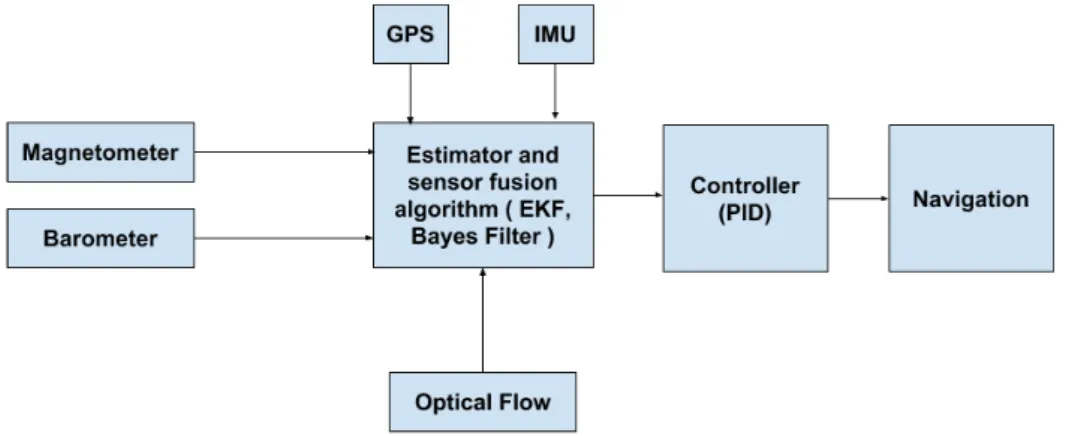
Navigation unit comprises of sensors and controllers which is required by the UAV for flying. It consists of fundamental parts required for navigating from one point to another. Fusing the input from sensors such as IMU, GPS, mag-netometer, and barometers are useful for estimating the position, velocity, acceleration, and orientation of the vehicle. This information is used by the UAV to provide the corresponding input to the controller for navigating to its destination. The control command is converted to the thrust which is applied to the motors by controllers such as proportional-integral-derivative (PID). This section introduces sensors such as IMU, GPS, and optical flow. It also introduces simple probabilistic model such as Bayes algorithm that can provide a good estimation. The foundation built with Bayes algorithm will be useful later when discussing Kalman filter and extended Kalman filter

which is more robust at estimation compared to Bayes algorithm and cur-rently used in many flight controllers. The navigation unit is summarized in figure 2.1.

Figure 2.1: Navigation Unit

2.1.1

Inertial Measurement Units (IMU)

IMU is a device that helps in estimating relative position, velocity, and ac-celeration of moving vehicles using gyroscopes and accelerometers. IMU is of two types: gimballed and stripped down. Gimballed IMU keeps mass in the horizontal position and is free to move in any direction. Stripped down IMU has fixed system connection which calculates orientation. The gyro-scope is used to measure changes in position and is built with technologies such as fiber optic, a ring laser, hemispherical resonator, and MEMS. Simi-larly, the accelerometer is used to measure external forces including gravity. The force is calculated based on the deflection of the mass. Despite being es-sential equipment for measuring motion, IMU inherits several problems such as random drift caused by measuring errors leading to short or long-term drift. Nevertheless, the problem of drift can be mitigated by fusing data from sensors like GPS using an appropriate filter such as Kalman filter [5]. It is commonly used in devices which requires estimating motions such as planes, cars, smartphones, robots, and drones.

2.1.2

Global Positioning System (GPS)

GPS is a satellite-based navigation system consisting of 24 satellites orbiting the earth. These satellites revolve around the earth every 12 hours trans-mitting signals containing a set of three values. Three values are a unique

number assigned to each satellite, position of the satellite in space and time of transmission of the signal. GPS receiver on the earth calculates its distance with respect to these satellites based on the signals received. For estimating the position on the surface of the earth with triangulation, signals from three or more satellites are needed. The number of signals from satellites increases to four or more for calculating elevation as well. However, the downside of GPS is its stringent requirement for the receiver to maintain a line of sight with the satellites which makes it useless for working in indoor environment, forest, and city with high structures[18]. Despite some shortcomings, GPS is popular and useful in outdoor robotics and drones, GIS data collection, surveying and mapping.

2.1.3

Optical Flow

To overcome shortcomings of GPS which require a direct line of sight to the satellites, visual odometry sensors such as optical flow can be used to estimate velocity and position using camera and range sensor. Optical flow camera has an ultrasonic sensor, Complementary Metal Oxide Semiconductor (CMOS) image sensor, and gyroscope as shown in figure 2.2. The ultrasonic sensor is used for scaling the distances whereas gyroscope is used for angular rate com-pensation. The CMOS image sensors enable optical flow sensors to operate indoor and outdoor environments with low light conditions. Furthermore, the distance measured by the ultrasonic sensor is also used for scaling optical flow values for calculating velocity. The calculation of the flow can be done using various methods such as phase correlation, block based, differential and discrete optimization methods.

Optical flow calculates the flow or motion of different points of interest in consecutive frames of video or images. One of the popular block-based method commonly used for flow calculation is the sum of absolute differences (SAD) [34]. SAD algorithm serves as the first step and measures a similarity between different image blocks. For calculating flow, these different image blocks will be the reference block of pixels of the current and preceding frame. The position of the match between these reference frames is selected and used for calculating flow value. Furthermore, subpixel refinement can also be done for better accuracy using bilinear interpolation.

Another prominently used differential based algorithm is Lucas-Kanade [67]. It uses affine model and image patches for flow field. It is less sensitive to noise but is a local method. Once the flow is calculated from the images, it can be used to estimate translational velocity. Translational velocity is calculated from two-dimensional flow field after scaling it to current scene and compensating angular rate. Thus, using optical flow gives an accurate

estimate of position and velocity. Optical flow is used for high estimation accuracy and in the absence of GPS signals.

Figure 2.2: Optical Flow sensor with CMOS image, gyroscope and ultrasonic[34]

.

2.1.4

Bayes Algorithm and Probabilistic Model

Drones cannot directly observe the real world; thus there is a need to esti-mate the motion so that they can localize themselves and move towards the destination. By getting feedback and reading from sensors, a drone can esti-mate its position against the known surroundings. State estimation is done based on position and velocity of the drone and map of the environment where the drone is operating. The estimation can be done in one of three ways which are control based, odometry based and velocity based. In control based estimation, robot estimates motion from the control commands issued to it. Similarly, odometry based are used for the systems with distance sen-sors such as wheel encoders, whereas, velocity based state estimation is used in the absence of wheel encoders. There are several algorithms and filters used for controlling and navigating the drones, and one of the basic filters is Bayes filter which is discussed in succeeding paragraphs.

Before jumping into the Bayes algorithm, it is required to understand how Bayes formulates sensor and motion model. Robot perceives its environment through its sensors and can be defined as in equation 2.1.

z =h(x) (2.1)

where,

z is sensor reading

h is sensor model (observation function)

x is world state

and sensor model. However, we can get the world state as well if we know the sensor reading by inverting the sensor model as shown in equation 2.2.

x=h−1(z) (2.2)

Similarly, based on the motion, state of the drone can be estimated. Belief state will be updated based on action or control command issued to the drone. It is defined in equation 2.3.

x0 =g(x, u) (2.3)

where,

x0 is current state

g is motion modeling

x is the previous state

u is executed action

The motion model is vague and prone to errors with the increase of time. However, it has a higher frequency and can update up to 500-1000 Hz com-pared to sensor model which has much lower update rate at 10-100Hz. Thus, the motion model can calculate the belief state at a higher frequency which can be corrected with sensors model. The sensor model is also not completely accurate and is often noisy and incomplete which makes the model partially wrong. Such a problem can be mitigated with the prior knowledge about the environment where the robot is operating, thus improving the estimate. This information can be used to verify the belief and estimates calculated from sensor and motion model. Thus, the estimation is done more in the proba-bilistic sense rather than trying to find the exact position [65]. Probaproba-bilistic models is represented as shown in equations 2.4 and 2.5.

P robabilistic sensor models=p(z|x) (2.4)

P robabilistic motion models=p(x0|x, u) (2.5) As shown in equation 2.6, input from different sensors can be fused which is also known as multi-modal models and is used to improve the accuracy of the estimation.

p(x|zvision, zultrasound, zIM U) (2.6) Understanding Markov assumption is also necessary for understanding the probabilistic models and is defined by two statements.

1. Sensor observations depend only on current state

2. Current state depends on current action and previous state

p(xt|x0:t−1, z1:t, u1:t) =p(xt|xt−1, ut) (2.8) With Markov assumption, the probabilistic state estimation estimates state of the dynamic system given the sequence of observations and actions, sensor model, action model and prior probability of the system. Such an estimation of the state is also called a belief.

Bel(xt) =p(xt|u1, z1, ..., ut, zt) (2.9) In motion model, it tries to calculate the probabilistic region of interest based on the motion. However, measurements are inaccurate which weakens the estimation, and increases the probable region for localizing drone. Thus, input from sensor model is used to correct the readings from motion model. Bayes filter algorithm can be summarized in two steps [58] which is given below.

Repeat for each time step, 1. Apply motion model

Bel0(xt) = X xt−1

P(xt|xt−1, ut)Bel(xt−1) (2.10) 2. Apply sensor model

Bel(xt) = (zt|xt)Bel 0

(xt) (2.11)

2.2

Obstacle Avoidance Unit

Similar to the navigation unit discussed in 2.1, obstacle avoidance unit is an integral part of a UAV. Though it is not required for a drone to fly, it en-sures the vehicle reaches the destination safely. UAV can sense and react to the environment both dynamic and static based on the input from this unit. While navigation unit concerns about reaching the destination through the shortest possible path, obstacle avoidance unit concerns about reaching the destination with short and safest path. It comprises range sensors such as lidar, radar, sonar and depth cameras. The input from these sensors is pro-vided to obstacle avoidance algorithms such as thresholding or vertical field histograms. This section introduces some of the range sensors and vertical field histograms algorithm for obstacle avoidance. The obstacle avoidance unit is summarized in 2.3.

Figure 2.3: Obstacle Avoidance Unit with corresponding components

2.2.1

Light Detection and Ranging (Lidar)

Light Detection and Ranging is a method for measuring ranges with a light in the form of pulsed laser. There are several lidar available commercially such as Garmin lidar lite [29], Velodyne lidar[25] and Rplidar[54]. For this thesis, Garmin lidar lite is used as obstacle avoidance sensor. The appli-cation of this sensor can be found around unmanned vehicles, robot, and drones for detecting range and proximity. The size of the device is compact with low power consumption which can be useful for autonomous vehicles. The communication with the sensors can be done either with I2C or PWM. Figure 2.4, 2.5 and 2.6 shows Garmin lidar lite, Velodyne lidar and Rplidar respectively.

2.2.2

Radio Detection and Ranging System (Radar)

Radar uses electromagnetic waves for finding the relative coordinate of the object in respect to its position. It works by radiating energy in UHF and microwave range, and monitoring the echo reflected back from the objects. The primary radar system consists of a transmitter which produces an elec-tromagnetic signal radiated into space through an antenna. This electromag-netic signal is either reflected back or reradiated when it strikes on objects. The reflected signals which are received by Radar antenna are processed to determine the position of objects[59]. The distance is calculated by multi-plying the speed of light with the time taken by signals to travel from the radar to the target.

2.2.3

Sound navigation and ranging (Sonar)

Unlike radar which is based on electromagnetic waves, sonar is based on sound waves. The detection of the object is based on the propagation of sound from target detector. There are two types of sonar, active and passive [24]. Active sonar system transmits waves which travel back to the receiver. However, in passive sonar system target is the source of energy propagating to the receiver. Distance to the object is calculated by the speed of sound in the medium multiplied by the time taken to traverse the distance.

2.2.4

Depth Camera

Depth camera provides an additional information of depth value in addition to common Red-Green-Blue (RGB) value for each pixel. Depth information gives drones or any other computer vision application capability to perceive three dimensions of its environment. The process of finding the depth it-self is usually done with stereoscopic vision in which two cameras are used. The camera can be used for not only perceiving the obstacles in the environ-ment where drones are operating but also for finding a safe path to navigate through the obstacles. Several depth cameras are available in the market such as Microsoft Kinect, Intel RealSense, and ZED stereo cameras. This thesis uses Realsense camera which is a depth camera developed by Intel and shown in the figure 2.7. The process of calculating depth is given by the equation 2.12. In the equation 2.12, the baseline is the separation between the two-identical infrared camera, the focal length is the focal length of the camera and disparity is the differences between the images obtained from two cameras.

Depth= (Baseline∗F ocalLength)/Disparity (2.12)

Figure 2.7: Intel Realsense R200 [53].

Figure 2.8: Intel Realsense R200 internals as provided in [53].

Figure 2.8 shows the interior of the camera which includes following com-ponents

1. Imaging ASIC onboard camera 2. Depth capture in VGA resolution 3. Class 1 Infrared laser projector system

The R200 camera provides several video streams such as color, depth and infrared. The difference between depth video streams and color video is based on what each pixel represents. The pixel in color video stream encodes RGB values whereas pixel in-depth video streams represent depth. The module consists of infrared laser projection system, two infrared cameras, and a full HD color imaging sensors. Per-pixel depth is calculated with stereo vision

technology in assistance with the infrared laser projector and the two infrared imaging sensors [40].

2.2.5

Polar Histogram/Vertical Field Histogram

Vertical Field Histogram is a method for finding the obstacles present on the navigation path of drone based on the input from range sensors creating a polar obstacle density as shown in figure 2.9. The world is modeled as a two-dimensional histogram grid which is updated continuously with distance data obtained from range sensors. The process of creating a world model involves two stage of data reduction which in turn has three level of data representations [10]. The first level of data representation involves continu-ously updating cartesian histogram grid in real time with range data from sensors. The second level of data representation involves constructing one-dimensional polar histogram(H) around drone’s momentary location. The third and last level of data representation is the command for navigating the drone.

Figure 2.9: Polar Obstacle Density [20]

Creation of Polar histogram The polar histogram H comprises of n

angular sectors each of width αas shown in figure 2.10. An active region C∗

which is a region drone currently sees is transformed such that each sector k

is holding a value hk. This value represents polar obstacle density (POD) in the direction of the sector k. Active region window moves with the vehicle

overlying a square region of ws∗ws cells in the histogram grid. Contents of active cells in the histogram grid are treated as obstacle vectors, the direction of which is determined by the angle between the cell and the Vehicle Center Point (VCP).

Figure 2.10: Vertical Field Histogram [10] showing the formation of polar obstacle densities in front of the vehicle.

Steering controller The next stage computes steering direction θ. The smooth polar histogram has peaks and valleys representing sectors with high and low PODs respectively. Valley with POD below a certain threshold is called as a candidate valley which can be used for navigating the drone. There can be more than one candidate valley to choose from, and the selection of appropriate valley is based on minimum deviation from the direction of the target. Valley may be comprised of multiple sectors, thus after selection of the valley suitable sector within that valley has to be chosen.

2.3

Artificial Intelligence

This thesis explores how AI can be used to assist obstacle avoidance and nav-igation which requires understanding different components of AI and how it can be used in UAV. In this section, the general concept of AI, search prob-lems, neural network, convolutional neural network, reinforcement learning

and deep reinforcement learning is introduced. It also discusses a software tool caffe and digits (Nvidia Deep Learning GPU Training System) for im-plementing the convolutional neural network. Finally, it summarizes current research ongoing on AI for drones. The architecture for AI used in this thesis is summarized in 2.11.

Figure 2.11: Aritificial Intelligence Unit showing different components in-volved for developing an intelligent system.

2.3.1

General Introduction to AI

Artificial intelligence has established itself as an integral part of robotics. The definition of AI can differ depending on its usability and field, but as defined in [50], it is designing of an intelligent agent which can interact with the environment and take action to maximize its success where an agent acts rationally to get the best outcome. AI can also be described as a search problem where an agent is trying to find the best possible solution out of several choices. Thus, local search problems such as hill climbing, adversarial search problems such as minimax and alpha-beta pruning and uninformed search such as A* or IDA* are part of the AI. Due to its vast nature, it has found applications in several fields such as speech recognition, handwriting recognition, machine translation, robotics, recommendation system, spam filtering, face detection, face recognition and autonomous driving. Some of the concepts of Artificial Intelligence is discussed in succeeding paragraphs.

Intelligent Agents An agent is capable of perceiving and taking action to attain some goals in an environment. AI tries to define a rational agent which can maximize its reward under different constraints such as limitations of computation power. Based on complexity, an agent can be of different types such as simple reflex agent, model-based reflex agent, goal-based agent and utility-based agent [56]. A simple reflex agent has no memory and selects an action based on current state only. This type of agent can work efficiently

only in the fully observable environment. A model-based agent has some memory and is operable in the partially observable environment. Goal-based agent understands its goals and knowledge of its environment which it uses to attain that goal. Finally, the utility-based agent has a utility function for measuring the performance of the agent. All the above agents can be gener-alized as learning agents who have four components learning, performance, critic and problem generation.

Environment The environment is where an agent performs an action. It is of several types such as fully observable or partially observable, deterministic or stochastic, episodic or sequential, static or dynamic, discrete or continuous, single agent or multi-agent and known or unknown.

Search Agents AI can be generalized as a search problem so an agent in AI is basically a search agent. Such agent is goal oriented and tries to identify series of actions to attain the defined goal. Search problem can be defined with an initial state, state space, action space, transition model, a test of goal and cost of the path. The initial state is where search agents start its search. Set of states that can be reached from the initial state is state space. Set of actions available to the agent is known as action space. Transition model defines if an agent can go from one state to another and what actions are required for such transition. Test of goal checks whether the defined goal is reached or not. Cost of the path is the total cost incurred to reach the goal.

Search can be Uninformed search or Informed search based on whether search agent has knowledge of the domain it is searching. In uninformed search, an agent has no information regarding searching criteria, thus, must search entire state space in a brute force manner. Some examples of such searches are breadth-first search, depth-first search, depth-limited search, iterative deepening and uniform cost search. However, an agent can have a knowledge of the domain through a heuristic function. The heuristic function measures the closeness of state to its goal. Such search is known as informed search and greedy best-first search, A* search, and Iterative Deeping A* (IDA*) search are some examples. All the searches discussed earlier are trying to find the best path by applying optimization globally. However, search can be local and local search is useful for optimizing complex problems.

Local Search The real-world problems are usually much complex and are not suitable to apply the generic global search approaches discussed above, instead, a search can be done locally by iteratively improving the utility.

Local search tries to keep a single current state and tries to improve it without maintaining a search tree. Thus, it has less memory and performs better in large state spaces. Some examples of local searches are hill climbing, simulated annealing, local beam search and genetic algorithms.

Adversarial Search Adversarial Search is used in multiagent competitive environments such as games. In games, there usually is an adversary not under the control of the agent acting to minimize the utility. Two popular adversarial searches are minimax and alpha-beta pruning. In minimax, there are usually two players one of them is trying to maximize its utility whereas the other one who is adversary is trying to minimize it. Alpha-beta pruning is like minimax but has better performance as it keeps track of two bounds for pruning the search space. Alpha is the largest value for maximum across visited state spaces and beta is the lowest value for minimum across visited children.

2.3.2

GPU Computing Platform

Graphics Processing Unit (GPU) is used for processing graphics. Processing of videos and images are highly parallel in nature such as mean subtraction from image involves subtraction of mean value from entire pixels of the im-age. For that reason, GPU was created to be a highly parallel system with hundreds of cores running thousands of threads. This support for the highly parallel system is realized to be highly efficient for computing parallel task such as training Neural network. Thus, GPU saw a rise in its demand re-cently with increased uses of AI. This thesis is using Jetson TX2 as a GPU computing device which is shown in figure 2.12.

Jetson TX2 is one of the dominant embedded AI computing device devel-oped by Nvidia which has 8 GB memory and 59.7 GB/s memory bandwidth. GPU architecture is Nvidia Pascal with 256 Compute Unified Device Archi-tecture (CUDA) cores. In addition to that, it has quad core 64-bit arm, eight processors. For interfacing the video, it has Camera Serial Interface (CSI), Universal Serial Bus (USB), High-Definition Multimedia Interface (HDMI) and gigabit ethernet port. It can support processing of up to 6 HD videos. Furthermore, it includes latest technology for deep learning and computer vision which makes it an ideal candidate for embedded AI computing. In ad-dition to reliable hardware resources, it comes with a platform that enables smooth implementation of Artificial intelligence. The difficulty to start devel-oping AI is very low with Jetson hardware and software resources. The SDK includes deep learning (tensorRT, cuDNN, Nvidia Digits workflow),

com-puter vision (Nvidia visionworks, OpenCV), GPU compute (Nvidia Cuda, Cuda libraries) and multimedia[52].

Figure 2.12: Nvidia Jetson TX2 model [52]

2.3.3

Neural Network

The neural network is a network of neurons arranged in several layers and dimensions. The fundamental part of any neural network is a neuron. Each neuron has a set of inputs, weights, biases and activation functions. The structure of the neuron is defined and shown in figure 2.13.

Input For the first layer, an input of a neuron will be data, but for hidden layers, it will be the output of the neuron in preceding layer.

Weights After receiving the inputs, neuron computes the weighted sum by assigning a parameter known as weight for multiplying with each input variable. Weights are an important parameter because the activation of a neuron depends on its value. Learning in the neural network means finding proper value for these weights parameters. During the first step of training, the weights should be initialized with some small random value but not zero.

Bias The weights are used for computing linear weighted sum of input; however, there might be a need for thresholding this value depending on the applications and data. Bias is a constant and is used to threshold the output of weighted sum. It can be positive or negative depending on which direction thresholding is needed. It is also another learnable parameter and is learned

over the course of training. The initialization of bias can be zero during training. Each neuron possesses a single bias to shift its weighted sum up or down.

Activation Function The summation of the weighted sum and bias mod-els a linear system. However, most of the real-life systems are nonlinear. In such a scenario, activation function provides a mechanism for representing a nonlinear system. The output of summation is fed into activation function which does the nonlinear transformation.

Output of Neuron It is the output of the activation function. For the hidden layers, this output is fed as input to succeeding layers. However, in the output layer, output calculates the weighted sum and provides a classification or regression data as per the application [38].

Figure 2.13: Single Neuron[38]

Activation Function

As discussed above, one of the fundamental parts of a neuron is its acti-vation function, in the absence of which neural network cannot represent anything more than a linear system[37]. The performance of neural network and training duration can be largely influenced by choice of the activation function[38]. Some of the popular activation functions are discussed below.

Sigmoid It is also known as logistic function and is represented by equation 2.13. Parameterawhich is a slope is important. When it approaches infinity, logistic sigmoid approaches threshold function, and when it approaches zero, the function has a large linear region between the threshold. It is continuous

and continuously differentiable.

f(v) = 1/(1 +e−av) (2.13) The problem with sigmoid function is that it saturates and kills the gradients. Furthermore, the output from the sigmoid functions are not zero-centered. Output value ranges from [0, 1]. Sigmoid function is shown in figure 2.14.

Figure 2.14: Sigmoid Function

Tanh The symmetric version of sigmoid function is tanh function which is represented by equation 2.14.

tanh(x) = (ex−e−x)/(ex+e−x) (2.14) This activation function overcomes the problem of sigmoid of not being zero centered. However, the problem of saturation persists. The value of such a function range from [-1, 1]. Tanh function is shown in figure 2.15.

ReLU It is getting more popular with deep neural network and is defined by equation 2.15.

f(x) =max(0, x) (2.15) ReLU helps in accelerating the convergence of stochastic gradient descent when compared with sigmoid and tanh. Implementation is quite straightfor-ward which is done by simply thresholding a matrix of activation at zero. However, it can be fragile during training and die. ReLU function is shown in figure 2.16.

Figure 2.15: Tanh

Figure 2.16: ReLU

Multilayer Perceptron

A single neuron can be used by itself for modeling some simple system. By stacking such neurons into multiple layers, a complex system can be represented, and such a network of neurons is known as multilayer perceptron. The first layer is called input layer, and no computation is done in this layer. The final layer is output layer which only does linear combinations of input from an earlier layer and has no nonlinear component. All the layers in between are the hidden layer. Each neuron in the hidden layer has the architecture like the one shown in figure 2.17.

Backpropagation

With no training, all the parameters such as weights and biases have random values or zeroes. Such a system does not represent anything. For making a neural network useful, it needs to undergo training so that all the parameters

Figure 2.17: Multilayer Perceptron [38]

such as weights and biases are properly updated to model the system. The first step of training is to initialize these parameters. The network will be incapable of representing much if all the weights in the network are initialized to zero. With zero initialization, the weighted summation of input will be zero, and all the neurons in each hidden layer will be learning the same thing [49]. Also, the choice of initialization affects the performance and time of convergence of training of a neural network.

During an initial phase of training, excitation of neurons is random gen-erating random output. For the supervised learning where labeled data is available, the difference between what is expected and what is generated can be observed. This difference between the expected output and real output is a loss. The losses over all the training examples are averaged by defin-ing a cost function which is used to update the parameters of the network. In a neural network, least square cost function is popular, where the sum of squared difference between the expected output and real output is calculated. Once a cost is calculated, weight is adjusted such that it will start favoring expected outcome. The process of updating weights and biases starts from output layer with stochastic gradient descent (SGD) method [37]. The pro-cess does not stop in the outermost layer but proceeds to the earlier layer until it reaches the first hidden layer. The name backpropagation is thus coined as the algorithm starts from the last layer and propagates backward to the first layer.

2.3.4

Convolutional Neural Network

Convolutional neural networks are used for image classification [43][42]. The way we store the image in the memory leads to loss of spatial information. Spatial information is lost because images are flattened and represented as an array of pixels in one-dimensional memory. When this representation is fed to the machine, it just sees a bunch of pixels. As a result, all the spatial

information present in the image is lost. CNN tries to preserve this spatial information by using filters which convolve with multiple pixels in a small window of 3x3, 5x5 or 7x7 sizes. Convolution is used for searching spatial features in images such as contours, lines, circles, honeycomb or any subtle features [19].

Comparison with Multilayer Perceptron (MLP)

Convolutional Neural Network is a variant of the multilayer perceptron. How-ever, unlike generic MLP, CNN has sparse connectivity and shared weights [22]. MLP has fully connected layers which means output from a layer is connected to all neurons in the subsequent layer, but CNN only has spatially contiguous connections. The learning parameters are weights in MLP, but CNN has two-dimensional filters. Each of these filters is used to convolve im-ages creating a two-dimensional output. The number of filters can be more than one generating three-dimensional output. Same weights of the filter are used to convolve entire image in contrast to MLP which has different weights for different input.

Like MLP, CNN has repetitive blocks of neurons creating 3D volumes of neurons. As shown in figure 2.18, a convnet has 3 dimensions. Different operations are happening in various stages of CNN which can be repeated over. Different operations of the convolutional neural network are described in the succeeding paragraphs.

Figure 2.18: Convolutional Neural Network Internal [38]

Input When dealing with images, the input will be Red-Green-Blue (RGB) pixels. Thus, the total size of input will be height ∗ width∗ 3. Taking an example of Canadian Institute for Advanced Research-10 (CIFAR-10)

datasets which has 32∗32 size images, the total number of input in a single image will be 32∗32∗3.

Conv Conv layer is a convolutional layer where spatial features are ex-tracted by convolving a part of an image with a filter. The weights of such filters are learnable parameters. However, the number of filters each conv layer has can vary with each filter trying to learn distinctive charac-teristics of an image. The output of conv layer will be three dimensions

height∗width∗(numOf F ilters). Padding can be done for keeping the same dimension along height and width. Taking an example of CIFAR-10, if we have 12 filters with proper padding in first conv layer receiving CIFAR-10 input, then the output will be 32∗32∗12.

Relu Relu is an activation function popular in deep learning which is al-ready discussed in section 2.3.3. The function is applied for each element from the output of CONV layer. There is no change in the size of output in this layer.

Pool If the same size of input is continued, the number of parameters will increase by many folds. The mechanism used to decrease the parameters for a deeper network is called pooling which helps in reducing the size of the input. Pooling also helps in improving the performance of the layer and decreasing the training time. It is due to this layer all the subtle features which are identified in initial stages gets dropped when size is decreased resulting in more specific features of an image getting identified in later stages. The common way of pooling is max pooling where the maximum value is selected from a window of fixed sizes such as 2∗2 or 3∗3. If 2∗2 is used in CIFAR-10 datasets, the size of the image will decrease to 16∗16∗12. This layer, however, doesn’t decrease the depth.

Fully connected Layer CNN extracts features from the images and uses them to classify. The process of features extraction and representation hap-pens before the fully connected layer which is used for classification. It is the last layer of CNN and uses Softmax or SVM for doing actual classifications [48].

2.3.5

Deep Learning with Nvidia DIGITS

Nvidia’s Deep Learning GPU Training System (Digits) [17] is an interactive platform for training deep neural network. It provides the facility of

visual-Figure 2.19: Convolutional Neural Network [38]

izing each step of deep learning. The platform is used for processing data, configuring the deep neural network, monitoring the training progress, visu-alizing the trained sets, monitoring the performance of the network in real time and managing multi GPU training. Performance of deep neural network can be monitored in real time.

Dataset Creation Dataset can be created and uploaded using Digits. Ad-ditionally, it provides information about the dataset such as how many train-ing samples are available and what kind of data they are.

Network Configuration It provides facility to select standard networks such as LeNet, Alexnet or GoogleNet. These default networks can be used for training or can be modified according to the need. Options for setting solver parameters are available such as training epochs, the interval of snapshots, interval for validation run, batch size, type of solvers such as Stochastic Gradient Descent (SGD), ADAGRAD or NAG and learning policy and rate.

Training Results It provides real-time monitoring of training performance and accuracy. The model can be discarded or modified if performance is poor but can be retained if we are getting satisfactory results.

Monitor Overfitting and Underfitting It provides the graph of train-ing and validation loss for each epoch. If the loss continues to decrease for training set while increasing for validation set, then the network has overfit-ted. However, if the loss is not increasing, but accuracy is also not improving, then the network is underfitting.

Deployment It provides an easy method to download the network and transfer to the deployment device which can be mobile, server or laptops [17]. In this thesis, deployment device used is Nvidia Jetson. Figure 2.20 summarizes the process of training and deploying using Nvidia DIGITS.

Figure 2.20: Training and deploying deep learning with DIGITS [17]

2.3.6

Caffe

Different frameworks are available for training and deploying deep neural networks such as Theano, Tensorflow, Torch, and Caffe. Each framework has their share of strengths and weaknesses, and it is out of the scope of this thesis to analyze each of them. For this thesis, Caffe is used as deep learning framework due to its low learning curve, wide acceptability, and permissive Berkeley Software Distribution (BSD) license [35]. It is developed in Berkeley Vision and Learning Center and is written in pure C++ with CUDA support which has the command line, Python and Matlab interfaces. In addition to providing deep learning framework, it also has an implementation for pre-processing and deployment. There are reference models, and examples as a part of the framework and plethora of trained models are available in model zoo[12]. Such models ease in developing the application through early prototyping, easy training and easy deploying.

For providing input, Caffe has support for LevelDB or Lightning Memory-Mapped Database (LMDB) database, Hierarchical Data Format 5 (HDF5) and raw image files. It also supports in-memory computation for python and C++ language. Data preprocessing such as creating LevelDB/LMDB from raw images, shuffling data to generate training and validation sets and generating mean-image can also be done with Caffe. It also includes data transformations tools such as image cropping, resizing, scaling, mirroring and mean subtraction.

training parameters in Caffe is done with the protobuf model format. The format is developed by Google which is strongly typed and human readable. Several loss functions are available for both classifications such as softmax and hinge loss, linear regression such as Euclidean loss and attributes/multi-classification such as sigmoid cross entropy loss. The available layer types are convolutional, pooling and normalization. Similarly, many activation functions such as ReLU, Sigmoid and Tanh are available.

After training, Caffe generates .caffemodel which can be quickly deployed. Furthermore, it provides support for detection with regional CNN and seg-mentation with fully connected CNN. The platform is easily extendable for python and C++ to add a new layer or loss function.

2.3.7

Reinforcement Learning (RL)

Reinforcement learning is another variant of learning where drone tries achiev-ing some task by trial. Unlike supervised learnachiev-ing, reinforcement learnachiev-ing does not have any labeled data. In the absence of labeled data and cost func-tions, reinforcement learning uses reward function. The reward is a quantita-tive measurement of the outcome of an action performed. As shown in figure 2.21, reinforcement learning has several components such as agent, environ-ment, action, reward, and observation. An agent is always trying to learn to achieve some goals. An environment is where such action is performed and can be observed by the agent. An action is a task performed by an agent to attain its goal. A reward is a scalar feedback signal indicating the perfor-mance level by the agent at any time step t. Observation is a state of the environment an agent can observe [6]. The agent always tries to get the best outcome by maximizing its reward function. The reward is cumulative, and an agent tries to maximize its cumulated reward. At each time step, there is an interaction between the agent and the environment. The agent executes an action, receives observation and scalar reward, whereas, the environment gets action, emits observations and rewards. RL agent has no information about the environment, but it learns about it through a continuous process of actions, observations, and rewards. The goal of an agent is to find the policy that maximizes the utility function. The policy is a series of actions and utility function governs the rewards function. Agent continually inter-acts with the environment which is unknown initially to learn more about it. For doing so, an agent must balance and perform two sets of opposing steps which are exploration and exploitation.

Figure 2.21: Reinforcement Learning

2.3.8

Deep Reinforcement Learning (DRL)

The deep reinforcement learning tries to leverage the concept of a deep neu-ral network with reinforcement learning. By representing the utility function as a deep neural network, deep reinforcement learning tries to solve com-plex problems. Much research is ongoing such as [55] and [39] for using deep reinforcement learning to fly drones autonomously. It is different from super-vised learning in that we do not have labeled datasets for training so that we can find errors and then back propagate them. Thus, the concept of policy gradient comes along. The rewards can be (0, +1, -1) which will modulate our gradient to 3 possible values. For zero reward, our weights remain the same.

2.3.9

AI for drone navigation

There is much ongoing research on using AI and auto navigation in drones. Few of the recent articles focused in the thesis are [55], [39], [30], [13] and [28]. The authors in [55] and [39] have used imitation learning for controlling the drones and avoiding the obstacles. Similarly, authors in [28], [13] and [30] have used feed-forward deep neural network for controlling the drones and avoiding the obstacles. The authors in [28] discuss creating a dataset from 11,500 crashes which are then used to train standard deep network. The network outputs binary classification and provides the information about how to prevent a crash. It is a simple self-supervised model which is also effective in an extremely cluttered environment. The authors in [13] provide a method of using a single forward facing camera which is fed into the trained CNN model for depth estimation. The trained model was tested in both real and

simulated environment with satisfactory results. Similarly, authors in [30] trained the drone to perceive forest trails with a single monocular camera using the deep neural network. Furthermore, the dataset used to train the drone is freely available for download, and it is the same dataset used in this thesis for experimentation. Through imitation learning and recurrent neural network, authors in [39] are trying to train the UAV to fly across the simulated room in a cluttered environment. Authors in [55] also used a similar approach with forward-looking camera and imitation learning to navigate in a forest and controlled indoor environment.

2.4

Summary

The chapter introduced the fundamental background for this thesis. It pre-sented the basic components, sensors and algorithms explored during the course of this thesis. The navigation unit is required for the drone to navi-gate from one point to another. Similarly, obstacle avoidance unit is required for safely navigating in the cluttered environments. The thesis will later pro-vide integration of some obstacle avoidance sensors such as Garmin lidar lite and Realsense camera r200. A short introduction to AI is also provided and current research on the field on a drone is also summarized. AI will be used later in this thesis for better understanding the nature of an obstacle through image segmentation and navigation. Understanding of current research and solutions in autonomous cars can help us understand autonomy in drones as well. Autonomous cars have already solved many complex problems of navigation and obstacle avoidance. Next chapter will explore in more details how autonomy works in cars.

Case Study: Autonomous Cars

Both automobile and technology companies such as Tesla, Google, Uber, Nissan, BMW, Ford, and Mercedes are all developing autonomous cars [47]. Many of these autonomous cars today have level 4 autonomy where an au-tonomous vehicle has complete control. These auau-tonomous cars can be a huge source of inspiration and knowledge for applying similar technology for drones. Thus, the thorough understanding of architecture and applications for autonomous cars is one of the research focus of this thesis.

As defined by National Highway Traffic Safety Administration of US, autonomous driving has five levels of autonomy [23]. The levels are differ-entiated based on the degree of control and autonomy the vehicle has. The first level, also known as level 0, is a level where the car has no control on its own and is entirely controlled by the driver. The degree of control by an autonomous system increases from level 1 to level 4, and the autonomous system finally takes complete control in level 4. Such a vehicle operating in level 4 has the responsibility of all activities related to driving and exe-cuting functionalities such as safety-critical functions, parking, starting and stopping. The ability to perceive the environment in real time based on the input from multiple sensors enables vehicle of such autonomy. Some popular sensors used in autonomous cars are lidars, GPS, IMU, cameras, sonars, and radars. These sensors are used in localizing the vehicle and making real-time decisions for navigation. The task of autonomous driving, however, requires a high computation power to process a massive volume of sensor data.

As provided in [45], any autonomous system can be considered to have three components as shown in figure 3.1.

1. Sensing 2. Perception