Spatial Interpolation based Cellular Coverage Prediction with Crowdsourced Measurements

Spatial Interpolation based Cellular Coverage

Prediction with Crowdsourced Measurements

Massimiliano Molinari

*

_{, Mah-Rukh Fida}

†

_{, Mahesh K. Marina}

†

_{and Antonio Pescape}

*

*

_{University of Napoli Federico II}

†

_{The University of Edinburgh}

ABSTRACT

Coverage extension and prediction has always been of great importance for mobile network operators. For coverage ex-tension, the empirical and analytical path loss models assist in better positioning of the infrastructure. However post-deployment coverage prediction can be more cost effectively enabled by crowdsourced measurements. Unlike drive test-ing, crowdsourced measurements along with spatial interpo-lation techniques can help generate coverage maps with less expense and labor. Using controlled measurements taken with commodity smartphones, we empirically study the ac-curacy of a wide range of spatial interpolation techniques, including various forms of Kriging, in different scenarios that capture the unique characteristics of crowdsourced surements (inaccurate locations, sparse and non-uniform mea-surements, etc.). Our results indicate that Ordinary Kriging is a fairly robust technique overall, across all scenarios.

CCS Concepts

•Networks→Network measurement; Mobile networks;

Keywords

Cellular coverage prediction; crowdsourced mobile network measurement; spatial interpolation

1.

INTRODUCTION

Prediction of network coverage is of vital importance to mobile network operators and service providers. Not only before but also after the deployment of network infrastruc-ture, the level of network coverage provided to various parts of region under consideration is measured on a regular ba-sis. This regular check is to determine any coverage holes produced due to construction of new buildings, highways Permission to make digital or hard copies of all or part of this work for personal or classroom use is granted without fee provided that copies are not made or distributed for profit or commercial advantage and that copies bear this notice and the full citation on the first page. Copyrights for components of this work owned by others than the author(s) must be honored. Abstracting with credit is permitted. To copy otherwise, or republish, to post on servers or to redistribute to lists, requires prior specific permission and/or a fee. Request permissions from [email protected].

C2B(1)D’15, August 17-21 2015, London, United Kingdom

c

2015 Copyright held by the owner/author(s). Publication rights licensed to ACM. ISBN 978-1-4503-3539-3/15/08. . . $15.00

DOI:http://dx.doi.org/10.1145/2787394.2787395

or changes in customer residential preferences. In order to maintain customer market and fulfil obligations towards the regulatory authorities, such as FCC and Ofcom, the cover-age holes thus diagnosed are dealt with either by changing antenna tilt, its height, power level or deployment of new base stations etc.

To extend coverage and to deploy additional infrastruc-ture, the traditional approach is to use analytical propagation models (e.g., Okumura-Hata, Longley-Rice irregular terrain model) [1]. Some empirical measurements may be needed for this approach and in developing the underlying models themselves (e.g., Okumura-Hata) to obtain fitted constants and for adjustments/corrections of model equations. How-ever to optimize the coverage, in operational phase, this ap-proach, exemplified by 3G coverage maps produced by Of-com in [2], is inherently inaccurate. A relatively newer and potentially more accurate approach to coverage prediction and mapping is based on geostatistics (e.g., [3–5]). It in-volves strategically collecting measurements (referred to as spatial sampling) and use of spatial interpolation techniques to predict values at unobserved locations. This type of cov-erage estimation via measurements and interpolation is pre-sented as an example application scenario of spatial big data in [6].

It is evident from the above description that both approaches to coverage prediction require measurements. Even to ob-tain measurements, there are two broad approaches. The traditional approach is drive testing (e.g., [7]), which is ex-pensive, labor intensive and time consuming. A more re-cent approach referred to as crowdsourcing (e.g., [8–11]) exploits end-user mobile devices as measurement sensors and the natural mobility of people carrying them for cost-effective and diverse spatiotemporal monitoring of mobile networks. Also, crowdsourced measurements reflect user perceived mobile performance, as they are obtained from end-user devices. To avoid the expense of drive tests, 3GPP has also been developing a specification called Minimiza-tion of Drive Tests (MDT) [12] for use in UMTS and LTE networks. MDT is also a crowdsourcing approach involving end-user devices for collecting measurements.

In this paper, we empirically study the effectiveness of a wide range of spatial interpolation techniques, including the widely used Kriging methods, for coverage prediction in the context of crowdsourced measurements. Specifically,

Figure 1: A taxonomy of spatial interpolation techniques based on [13].

crowdsourced measurements have certain unique character-istics, including: inaccurate locations of measurements; non-uniform and sparse set of measurements. We examine the impact of these different characteristics of crowdsourced mea-surements on the accuracy of spatial interpolation techniques, which has not been done before to the best of our knowledge. Our analysis results show that prediction error with spatial interpolation techniques is impacted by different crowdsourced measurement characteristics with Ordinary Kriging emerg-ing as a fairly robust technique overall.

The rest of the paper is structured as follows. Next sec-tion provides a brief overview of different spatial interpola-tion techniques and discusses related work. Following sec-tions, respectively, examine the impact of location inaccu-racy, measurement distribution and density on the accuracy of different spatial interpolation techniques. Section 6 con-cludes the paper.

2.

BACKGROUND

2.1

Spatial Interpolation Techniques

Pringle [13] presents a taxonomy of spatial interpolation techniques which we summarize in Figure1. There are mainly two types of interpolation methods, i.e. global and local in-terpolators. The former use all the available data whereas the latter use only the information in the vicinity of the point be-ing estimated. Interpolation methods can be exact or inexact. The predicted value of the exact interpolator is similar to the measured value; inexact interpolators remove this constraint and produce a smoother surface. Interpolation methods can be also categorized as deterministic or stochastic. Unlike deterministic, stochastic methods provide uncertainty esti-mates.

Below we outline the different spatial interpolation tech-niques considered in this paper.

• Krigingis a class of local interpolation techniques that are quite commonly used to address spatial prediction problems in the context of mining, hydrogeology, nat-ural resources, environmental science, etc.. The

ba-sic idea of Kriging is to estimate data at a point based on regression of observed surrounding values of that point weighted according to the spatial correlation of the field under study [14].

• Splines. These interpolators consist of a number of sections, and each fits to a small number of points so that each of the sections join up at points referred to as break points. We have analyzed the most common splines: bilinear and bicubic.

• Weighted Moving Average.This technique, exempli-fied by Inverse Distance Weighting (IDW), estimates data value for a point by calculating an inverse-distance based weighted average of the points within a search radius.

• Thiessen Polygons (THI)build polygons around each sample point; all points within a polygon are assumed to have the same data values as the sample point in the middle.

• LOESS Surfaces.LOcally wEighted Scatter plot Smooth (LOESS) performs two steps for each data point: (1) computes the regression weights for each data point in the so-calledspan, where the span controls the size of the neighborhood; (2) a weighted linear least squares regression is then performed with a second order poly-nomial.

• Trend Surfaces. A Trend Surface (TR-SRF) is basi-cally a 3D, linear or higher order, regression surface.

• Classification. In Classification (CLSF), the key idea is to infer the values of one variable attribute based upon the knowledge of the values of another attribute. The basic assumption is that the value of the variable of interest is strongly influenced by another variable that can be used to classify the study area into zones.

2.2

Related Work

There are several studies that have used Kriging for cov-erage prediction in wireless networks. In [15], Konak es-timates path loss in wireless LANs using Ordinary Kriging (OK) by defining the distance between two points as their Euclidean distance plus a term that represents the set of ob-stacles between the points. In [3], Phillips et al. use OK on a 2.5 GHz WiMax network setting, finding it to produce radio environment maps that are more accurate and informative than both explicitly tuned path loss models and basic fitting approaches.

In [16] and [17] Kolyaie et al. use drive testing to col-lect signal strength measurements, and compare the perfor-mance of empirical models and spatial interpolation tech-niques. Specifically, they use the Okumura-Hata empirical model, a common model used for cellular system planning and management. They evaluated its accuracy in compari-son with IDW and two Kriging variants: Ordinary Kriging (OK) and Universal Kriging (UK). Though Okumura-Hata empirical model was seen to yield better results than IDW,

OK and UK provided best prediction results. Our work is in a similar spirit with one crucial difference: we focus on the issues that arise when dealing with measurements obtained via crowdsourcing whereas Kolyaie et al. employed drive testing as the measurement approach.

In [4], Sayrac et al. propose Bayesian spatial interpola-tion for coverage analysis in cellular networks, specifically focusing on coverage hole prediction. Kitanidis’ Bayesian Kriging (BK) interpolation method is used which automati-cally calculates the interpolation model parameters through a process of sub-settings and simulations. The main disad-vantage of this method is its high computational complexity. In [5], Braham et al. consider a variant of Kriging called Fixed Rank Kriging (FRK), which is aimed at reducing the Kriging complexity. In fact, the computational complexity of Kriging isO(n3_{), wherenis the number of measurements.} The authors in [5] argue that FRK can reduce this compu-tational complexity while keeping an acceptable prediction error.

2.3

Data Collection and Methodology

For the purposes of this study, we rely on measurement data collected in a controlled manner using a custom An-droid app to obtain measurement information (GPS/network location, mobile network information, location area code, cell ID, signal strength in ASU1) along with exact measure-ment location manually inputted by the user.

Considering different scenarios that capture crowdsourced measurement characteristics, we study the accuracy with dif-ferent spatial interpolation techniques including various Krig-ing variants (OK, UK, BK and FRK) and other techniques outlined above.

To quantify accuracy of different interpolation schemes, we consider two standard metrics: Mean Absolute Percent-age Error (MAPE) and Root Mean Square Error (RMSE) values (in ASU). We considered two different testing meth-ods: leave-one-out-cross-validation (LOOCV) and calibration-and-validation (C&V); in the latter case, two-thirds of mea-surements are used to make a prediction in the remaining one-third. Unless otherwise mentioned, we report results for MAPE using the C&V method; other combinations yield similar results and are omitted for the sake of brevity.

In using Kriging methods, we have examined the appro-priate semivariogram model to use, model parameters, etc. Here we report on this investigation for basic and common form of Kriging called Ordinary Kriging (OK). For the pur-poses of this specific investigation, we collected 100 sig-nal strength measurements each in three different environ-ments: a friendly, an urban, and an indoor environment. We assume that an environment isfriendlyif the signal propa-gation is not very challenged having few physical obstacles (e.g., parks and rural areas). An environment isurbanif the signal propagation is more challenged, due to the existence of buildings and other obstacles (e.g., built environments of cities). Note that bothfriendlyandurbanare outdoor. As for

1_{ASU stands for arbitrary strength unit. Signal strength in ASU is on an}

integer scale and is linearly related to signal strength in dBm.

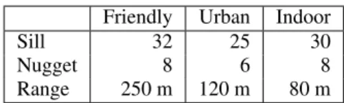
Friendly Urban Indoor

Sill 32 25 30

Nugget 8 6 8

Range 250 m 120 m 80 m

Table 1: Approximate variogram model parameters in the three environments.

indoorenvironments, the signal propagation is highly chal-lenged by walls and other obstacles between the base station and the user equipment.

First, we briefly comment on the various underlying as-pects of OK (semivariogram model, isotropy vs. anisotropy, model parameters); results omitted due to space limitations. While deciding about an appropriate empirical variogram model we found that exponential model followed by pen-taspherical leads to lower prediction error in all the envi-ronments; consistent with results shown in other works in the literature, such as [16]. Signal propagation in cellu-lar networks is an anisotropic phenomenon for several rea-sons (e.g. antenna geometries, cell sectors, etc.). How-ever we found that Kriging works better with an isotropic model. We believe that this might be because several over-lapping anisotropic phenomena together appear as an almost isotropic phenomenon.

Lastly, we notice that model parameters are actually influ-enced by the kind of environment. Table1shows the approx-imate variogram parameters in the three environments. Sill and nugget values are similar, where as the ranges are very different. The friendly environment has the largest range. It means that signal strength values show a remarkable cor-relation even if they are further away than in an urban en-vironment, where buildings obstruct signal propagation. In an indoor environment, the signal propagation is even more challenged, so it is unlikely that far away points are still cor-related.

3.

IMPACT OF LOCATION INACCURACY

Crowdsourcing based measurement exploits data obtained via commodity smartphones and the built-in mechanisms to obtain the device location. However localization mecha-nisms are imperfect and can result in highly inaccurate lo-cations in some cases. Therefore, a signal strength value es-timated to be taken at locations1, might have actually been observed ats2, wheredist(s1, s2)may be greater than a cer-tain tolerance threshold. This can clearly lead to mispredic-tion problems. In this secmispredic-tion we look into this problem, fo-cusing on the outdoor urban environment and the commonly used mechanism in smartphones for outdoor localization re-lying on GPS.

To assess the effect of GPS inaccuracies on the accuracy with different spatial interpolation techniques, we took a to-tal of 75 measurements of signal strength values within a small area in the city of Edinburgh; for each measurement, we stored both the actual and location reported by the phone GPS. We find that in our measurements the difference be-tween GPS and actual locations were, on average, of 18

me-Figure 2: Impact of location inaccuracy on MAPE performance of different spatial interpolation techniques.

Figure 3: Prediction errors in terms of MAPE with different interpolation schemes for uniform spatial distribution of

measurements.

ters. We evaluated the accuracy of the prediction with GPS based location and actual location. Figure 2 displays the prediction errors in terms of MAPE with different interpo-lation techniques withActualas well asGP Sbased loca-tions. We see that some techniques are more affected than others. Splines-Bicubic, Thiessen Polygons and LOESS re-gressions are negatively impacted. For LOESS, we only show the result with the span value that yields the best pre-diction — results with other span values are similar to that with Bicubic. This is no surprise, since they strongly rely on the notion of neighboring points to make a prediction. As for Kriging-based techniques, OK and UK yield better pre-dictions even in presence of location inaccuracies while BK and FRK can be seen to be more sensitive to location inac-curacy. As per other techniques, IDW and Trend surfaces are also only slightly affected; this is as expected since they mainly rely on regional trends.

4.

SPATIAL DISTRIBUTION OF

MEA-SUREMENTS

With crowdsourcing based measurement, the spatial dis-tribution of participant devices may not be uniform in the re-gion of interest. In this section, we consider such scenarios with measurements distributed non-uniformly in space. To serve as a reference, we first consider a more ideal scenario with uniformly distributed measurements in space; here the goal of spatial interpolation techniques is to estimate the data in the gaps which are unmeasured.

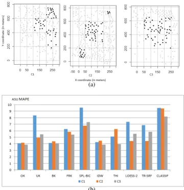
(a)

(b)

Figure 4: (a) Clustered measurement scenarios; (b) Prediction errors in terms of MAPE in each of the clustered measurement

scenarios.

4.1

Uniform Distributed Measurements

To assess properties and performance of spatial interpola-tion techniques when measurements are uniformly distributed, we use C&V approach as before but in such a way that both calibration and validation points are chosen randomly andunif ormly throughout the interest area. Specifically, we consider a urban outdoor open space in a park and use 479 measurements in total of which 420 measurements were used for calibration and rest for validation. The prediction error results are shown in Figure 3. The differences sev-eral of the schemes are somewhat negligible in this scenario. Exceptions to this conclusion are Splines and Classification, which perform very poorly. Like before, a few of the schemes like BK, FRK and Thiessen Polygons yield predictions with higher errors but not as high as Splines and Classification.

4.2

Non-Uniformly Distributed

Measure-ments

We now consider the more realistic case of non-uniformly distributed measurements in space. We use measurements from the same park environment but taken in a spatially non-uniform manner, specifically to reflect clustered measure-mentsandmeasurements with holes.

4.2.1

Clusters

Clustered scenarios are shown in Figure4(a), with black dots showing positions of calibration data and gray dots in-dicating validation points; the number of calibration points

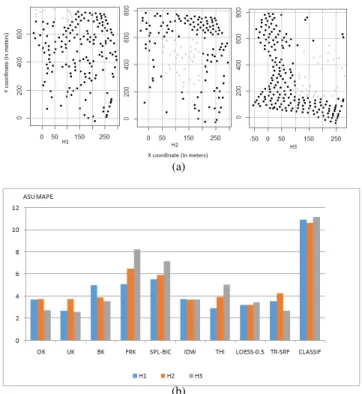
(a)

(b)

Figure 5: (a) Scenarios with measurement holes; (b) Prediction errors in terms of MAPE in each of the measurement hole

scenarios.

is around 50 in all three scenarios and there are at least 100 validation points in each of the scenarios.

We find that prediction errors are widely different for dif-ferent span values with LOESS. Though not shown in Fig-ure4(b), LOESS with span values less than 0.75 yield quite erroneous results. As per the other schemes, we see that OK and IDW in particular consistently give lower predic-tion errors across all scenarios, whereas other schemes like Splines-Bicubic and Classification give worse results as be-fore.

4.2.2

Holes

Scenarios with measurement holes are shown in Figure 5(a) with black dots indicating calibration points and rest are validation points where predicted values are compared with actual values to compute the errors and MAPE. As with clustered scenarios, here we consider scenarios with differ-ent forms of holes: a smaller corner hole, a large middle hole and a bigger side hole surrounded from three sides. Predic-tion errors in each of these scenarios is shown in Figure5 (b). As with clustered scenarios, the nature of the holes in-fluences the prediction errors with different schemes. We also note that prediction errors are higher in clustered and hole scenarios compared to the initial case with spatial uni-form measurements.

5.

MEASUREMENT DENSITY

In this section we want to assess the impact of

measure-Figure 6: Impact of measurement density on MAPE values for Kriging techniques, IDW, THI and TR-SRF.

Figure 7: Impact of measurement density on MAPE values for LOESS Surfaces, Classification and Bicubic Splines.

ment density on the prediction. For analysis we collected about 500 measurements in a park in Edinburgh and then se-lected 479 measurements out of these so as to have similar density throughout the area. We used 59/479 measurements as validation dataset and the remaining 420/479 as initial cal-ibration dataset. The size of the calcal-ibration dataset is then gradually decreased in steps to obtain different density val-ues. We consider 9 steps. In the initial one (step 1), we have about 14 measurements per squared hectare. In the last (step 9), we have only about one.

We show the prediction error results with varying den-sity in two graphs. Figure6focuses on Kriging techniques, IDW and Thiessen Polygones and trend surfaces, whereas results with LOESS, Splines and Classification are shown in Figure7. We observe that for most of the schemes, pre-diction error increases as measurement density decreases as one would expect. Some of the poorly performing schemes from earlier sections like Classification, Splines, FRK and BK still yield poor results largely regardless of measure-ment density. Prediction error gets really worse for low mea-surement densities with some of the schemes (e.g., LOESS, FRK). Though not shown in Figure7to avoid clutter, higher span values with LOESS (e.g., span value of 2) are more ro-bust at low measurement densities but come with somewhat higher prediction errors at higher measurement densities; the opposite holds for lower span values – we show the result with lowest span value of 0.3. Overall, we find OK and IDW to be most robust schemes across all measurement densities.

6.

CONCLUSIONS

In this paper, we have experimentally studied spatial inter-polation based cellular coverage prediction in the context of crowdsourced measurements. The crowdsourced measure-ment approach is cost effective compared to the traditional drive testing but comes with certain characteristics that intro-duce noise or make coverage prediction harder. Using con-trolled measurements taken using commodity smartphones in an urban environment, we have evaluated the accuracy of different spatial interpolation techniques, including various forms of Kriging, in several scenarios capturing unique char-acteristics of crowdsourced measurements. Our results show that basic form of Kriging called Ordinary Kriging generally performs well even when measurements are spatially non-uniformly distributed and when the measurement density is very low.

A possible aspect for future work is to develop a holis-tic framework that automaholis-tically selects the best prediction technique based on the measurement distribution, environ-mental information, measurement density, etc. Though we assumed a uniform random collection of measurements, we believe that improved results can be obtained by determin-ing an appropriate initial sampldetermin-ing pattern accorddetermin-ing to the region under study as proposed by Zio et al. [18] for envi-ronmental surveys. A suitable initial sampling design with a representative sampling size can minimize burden on the users and the systems for drawing and manipulating crowd-sourced measurements. Finally, better results can be achieved by designing an optimal second-phase sampling scheme for further minimization of prediction errors.

7.

REFERENCES

[1] C. Phillips, D. Sicker, and D. Grunwald. A Survey of Wireless Path Loss Prediction and Coverage Mapping Methods.IEEE Communications Surveys & Tutorials, 15(1), 2013.

[2] Ofcom. 3G Coverage Maps.http://licensing.ofcom. org.uk/binaries/spectrum/mobile-wireless-broadband/ cellular/coverage_maps.pdf, July 2009.

[3] C. Phillips, M. Ton, D. Sicker, and D. Grunwald. Practical Radio Environment Mapping with

Geostatistics. InProc. IEEE International Symposium on Dynamic Spectrum Access Networks (DySPAN), 2012.

[4] B. Sayrac, A. Galindo-Serrano, S. B. Jemaa, J. Riihijarvi, and P. Mahonen. Bayesian Spatial Interpolation as an Emerging Cognitive Radio Application for Coverage Analysis in Cellular Networks.Transactions on Emerging

Telecommunications Technologies, 24(7–8), 2013.

[5] H. Braham, S.B. Jemaa, B. Sayrac, G. Fort, and E. Moulines. Low Complexity Spatial Interpolation For Cellular Coverage Analysis. InProc. IEEE International Symposium on Modeling and Optimization in Mobile, Ad Hoc, and Wireless Networks (WiOpt), 2014.

[6] C. Jardak, P. Mahonen, and J. Riihijarvi. Spatial Big Data and Wireless Networks: Experiences,

Applications, and Research Challenges.IEEE Network, 28(4), 2014.

[7] C. N. Pitas, A. D. Panagopoulos, and P. Constantinou. Speech and Video Telephony Quality Characterization and Prediction of Live Contemporary Mobile

Communication Networks.Wireless Personal Communications, 69(1), 2012.

[8] Open Signal Inc.http://opensignal.com/.

[9] S. Sen, J. Yoon, J. Hare, J. Ormont, and S. Banerjee. Can they hear me now?: A Case for a Client-Assisted Approach to Monitoring Wide-Area Wireless Networks. InProc. ACM Internet Measurement Conference (IMC), 2011.

[10] J. Sommers and P. Barford. Cell vs. WiFi: On the Performance of Metro Area Mobile Connections. In Proc. ACM Internet Measurement Conference (IMC), 2012.

[11] A. Nikravesh, D. R. Choffnes, E. Katz-Bassett, Z. M. Mao, and M. Welsh. Mobile Network Performance from User Devices: A Longitudinal, Multidimensional Analysis. InProc. Passive and Active Measurement (PAM) Conference, 2014.

[12] J. Johansson, W. A. Hapsari, S. Kelley, and G. Bodog. Minimization of Drive Tests in 3GPP Release 11. IEEE Communications, 50(11), 2012.

[13] D. J. Pringle. Spatial Interpolation Techniques.

http://www.nuim.ie/staff/dpringle/gis/gis09.pdf. [14] M. A. Oliver and R. Webster. A Tutorial Guide to

Geostatistics: Computing and Modelling Variograms and Kriging.Catena, 113, 2014.

[15] A. Konak. Estimating Path Loss in Wireless Local Area Networks using Ordinary Kriging. InProc. Winter Simulation Conference, 2010.

[16] S. Kolyaie and M. Yaghooti. Evaluation of

Geostatistical Analysis Capability in Wireless Signal Propagation Modeling. InProc. 11th International Conference on GeoComputation, 2011.

[17] S. Kolyaie, M. Yaghooti, and G. Majidi. Analysis and Simulation of Wireless Signal Propagation applying Geostatistical Interpolation Techniques.Archives of Photogrammetry, Cartography and Remote Sensing, 22:261–270, 2011.

[18] S. D. Zio, L. Fontanella, and L. Ippoliti. Optimal Spatial Sampling Schemes for Environmental Surveys. Environmental and Ecological Statistics, 11:397–414, 2004.