Randomised Language Modelling for Statistical Machine Translation

Proceedings of the 45th Annual Meeting of the Association of Computational Linguistics, pages 512–519,

Randomised Language Modelling for Statistical Machine Translation

David Talbot and Miles Osborne School of Informatics, University of Edinburgh

2 Buccleuch Place, Edinburgh, EH8 9LW, UK

[email protected], [email protected]

Abstract

A Bloom filter (BF) is a randomised data structure for set membership queries. Its space requirements are significantly below lossless information-theoretic lower bounds but it produces false positives with some quantifiable probability. Here we explore the use of BFs for language modelling in statis-tical machine translation.

We show how a BF containingn-grams can enable us to use much larger corpora and higher-order models complementing a con-ventionaln-gram LM within an SMT sys-tem. We also consider (i) how to include ap-proximate frequency information efficiently within a BF and (ii) how to reduce the er-ror rate of these models by first checking for lower-order sub-sequences in candidate n -grams. Our solutions in both cases retain the one-sided error guarantees of the BF while taking advantage of the Zipf-like distribution of word frequencies to reduce the space re-quirements.

1 Introduction

Language modelling (LM) is a crucial component in statistical machine translation (SMT). Standard n -gram language models assign probabilities to trans-lation hypotheses in the target language, typically as smoothed trigram models, e.g. (Chiang, 2005). Al-though it is well-known that higher-order LMs and models trained on additional monolingual corpora can yield better translation performance, the

chal-lenges in deploying large LMs are not trivial. In-creasing the order of ann-gram model can result in an exponential increase in the number of parameters; for corpora such as the English Gigaword corpus, for instance, there are 300 million distinct trigrams and over 1.2 billion 5-grams. Since a LM may be queried millions of times per sentence, it should ideally side locally in memory to avoid time-consuming re-mote or disk-based look-ups.

Against this background, we consider a radically different approach to language modelling: instead of explicitly storing all distinctn-grams, we store a randomised representation. In particular, we show that the Bloom filter (Bloom (1970); BF), a sim-ple space-efficient randomised data structure for rep-resenting sets, may be used to represent statistics from larger corpora and for higher-ordern-grams to complement a conventional smoothed trigram model within an SMT decoder.1

The space requirements of a Bloom filter are quite spectacular, falling significantly below information-theoretic error-free lower bounds while query times are constant. This efficiency, however, comes at the price of false positives: the filter may erroneously report that an item not in the set is a member. False negatives, on the other hand, will never occur: the error is said to beone-sided.

In this paper, we show that a Bloom filter can be used effectively for language modelling within an SMT decoder and present thelog-frequency Bloom filter, an extension of the standard Boolean BF that

1

For extensions of the framework presented here to stand-alone smoothed Bloom filter language models, we refer the reader to a companion paper (Talbot and Osborne, 2007).

takes advantage of the Zipf-like distribution of cor-pus statistics to allow frequency information to be associated with n-grams in the filter in a space-efficient manner. We then propose a mechanism, sub-sequence filtering, for reducing the error rates of these models by using the fact that ann-gram’s frequency is bound from above by the frequency of its least frequent sub-sequence.

We present machine translation experiments us-ing these models to represent information regardus-ing higher-order n-grams and additional larger mono-lingual corpora in combination with conventional smoothed trigram models. We also run experiments with these models in isolation to highlight the im-pact of different order n-grams on the translation process. Finally we provide some empirical analysis of the effectiveness of both the log frequency Bloom filter and sub-sequence filtering.

2 The Bloom filter

In this section, we give a brief overview of the Bloom filter (BF); refer to Broder and Mitzenmacher (2005) for a more in detailed presentation. A BF rep-resents a setS = {x1, x2, ..., xn}with nelements

drawn from a universeU of sizeN. The structure is attractive whenN n. The only significant stor-age used by a BF consists of a bit array of sizem. This is initially set to hold zeroes. To train the filter we hash each item in the setktimes using distinct hash functions h1, h2, ..., hk. Each function is

as-sumed to be independent from each other and to map items in the universe to the range1tomuniformly at random. Thek bits indexed by the hash values for each item are set to 1; the item is then discarded. Once a bit has been set to 1 it remains set for the life-time of the filter. Distinct items may not be hashed to k distinct locations in the filter; we ignore col-lisons. Bits in the filter can, therefore, besharedby distinct items allowing significant space savings but introducing a non-zero probability of false positives at test time. There is no way of directly retrieving or ennumerating the items stored in a BF.

At test time we wish to discover whether a given item was a member of the original set. The filter is queried by hashing the test item using the same k

hash functions. If all bits referenced by thekhash values are 1 then we assume that the item was a member; if any of them are 0 then weknowit was

not. True members are always correctly identified, but a false positive will occur if allkcorresponding bits were set by other items during training and the item was not a member of the training set. This is known as aone-sided error.

The probability of a false postive,f, is clearly the probability that none ofkrandomly selected bits in the filter are still 0 after training. Lettingp be the proportion of bits that are still zero after thesen ele-ments have been inserted, this gives,

f = (1−p)k.

Asnitems have been entered in the filter by hashing eachktimes, the probability that a bit is still zero is,

p0 =

1− 1

m kn

≈e−knm

which is the expected value of p. Hence the false positive rate can be approximated as,

f = (1−p)k≈(1−p0)k ≈1−e−knm

k .

By taking the derivative we find that the number of functionsk∗that minimizesf is,

k∗= ln 2·m

n.

which leads to the intuitive result that exactly half the bits in the filter will be set to 1 when the optimal number of hash functions is chosen.

The fundmental difference between a Bloom fil-ter’s space requirements and that of any lossless rep-resentation of a set is that the former does not depend on the size of the (exponential) universe N from which the set is drawn. A lossless representation scheme (for example, a hash map, trie etc.) must de-pend onN since it assigns a distinct representation to each possible set drawn from the universe.

3 Language modelling with Bloom filters

Algorithm 1Training frequency BF Input: Strain,{h1, ...hk}andBF =∅

Output:BF

for allx∈ S_traindo

c(x)←frequency ofn-gramxinStrain qc(x)←quantisation ofc(x)(Eq. 1)

forj = 1toqc(x)do

fori= 1tokdo

hi(x)←hash of event{x, j}underhi

BF[hi(x)]←1

end for end for end for

return BF

3.1 Log-frequency Bloom filter

The efficiency of our scheme for storing n-gram statistics within a BF relies on the Zipf-like distribu-tion ofn-gram frequencies in natural language cor-pora: most events occur an extremely small number of times, while a small number are very frequent.

We quantise raw frequencies, c(x), using a loga-rithmic codebook as follows,

qc(x) = 1 +blog_bc(x)c. (1)

The precision of this codebook decays exponentially with the raw counts and the scale is determined by the base of the logarithmb; we examine the effect of this parameter in experiments below.

Given the quantised countqc(x)for ann-gramx, the filter is trained by entering composite events con-sisting of then-gram appended by an integer counter

jthat is incremented from 1 to qc(x)into the filter. To retrieve the quantised count for ann-gram, it is first appended with a count of 1 and hashed under thekfunctions; if this tests positive, the count is in-cremented and the process repeated. The procedure terminates as soon as any of thekhash functions hits a 0 and the previous count is reported. The one-sided error of the BF and the training scheme ensure that the actual quantised count cannot be larger than this value. As the counts are quantised logarithmically, the counter will be incremented only a small number of times. The training and testing routines are given here as Algorithms 1 and 2 respectively.

Errors for the log-frequency BF scheme are one-sided: frequencies will never be underestimated.

Algorithm 2Test frequency BF

Input:x,M AXQCOU N T,{h1, ...hk}andBF

Output: Upper bound onqc(x)∈ Strain

forj= 1toM AXQCOU N T do

fori= 1tokdo

hi(x)←hash of event{x, j}underhi

if BF[hi(x)] = 0then

return j−1

end if end for end for

The probability of overestimating an item’s fre-quency decays exponentially with the size of the overestimation errord(i.e. asfdfor d > 0) since each erroneous increment corresponds to a single false positive and d such independent events must occur together.

3.2 Sub-sequence filtering

The error analysis in Section 2 focused on the false positive rate of a BF; if we deploy a BF within an SMT decoder, however, the actual error rate will also depend on the a priori membership probability of items presented to it. The error rateErris,

Err=P r(x /∈Strain|Decoder)f.

This implies that, unlike a conventional lossless data structure, the model’s accuracy depends on other components in system and how it is queried.

We take advantage of the monotonicity of then -gram event space to place upper bounds on the fre-quency of ann-gram prior to testing for it in the filter and potentially truncate the outer loop in Algorithm 2 when we know that the test could only return pos-tive in error.

Specifically, if we have stored lower-order n -grams in the filter, we can infer that ann-gram can-not present, if any of its sub-sequences test nega-tive. Since our scheme for storing frequencies can neverunderestimate an item’s frequency, this rela-tion will generalise to frequencies: ann-gram’s fre-quency cannot be greater than the frefre-quency of its least frequent sub-sequence as reported by the filter,

c(w1, ..., wn)≤min{c(w1, ..., wn−1), c(w2, ..., wn)}.

3.3 Bloom filter language model tests

A standard BF can implement a Boolean ‘language model’ test: have we seen some fragment of lan-guage before? This does not use any frequency in-formation. The Boolean BF-LM is a standard BF containing all n-grams of a certain length in the training corpus,Strain. It implements the following

binary feature function in a log-linear decoder,

φbool(x)≥δ(x∈ Strain)

Separate Boolean BF-LMs can be included for different order n and assigned distinct log-linear weights that are learned as part of a minimum error rate training procedure (see Section 4).

Thelog-frequency BF-LMimplements a multino-mial feature function in the decoder that returns the value associated with ann-gram by Algorithm 2.

φlogfreq(x)≥qc(x)∈ Strain

Sub-sequence filtering can be performed by using the minimum value returned by lower-order models as an upper-bound on the higher-order models.

By boosting the score of hypotheses containingn -grams observed in the training corpus while remain-ing agnostic for unseenn-grams (with the exception of errors), these feature functions have more in com-mon with maximum entropy models than conven-tionally smoothedn-gram models.

4 Experiments

We conducted a range of experiments to explore the effectiveness and the error-space trade-off of Bloom filters for language modelling in SMT. The space-efficiency of these models also allows us to inves-tigate the impact of using much larger corpora and higher-order n-grams on translation quality. While our main experiments use the Bloom filter modelsin conjunction with a conventional smoothed trigram model, we also present experiments with these mod-els in isolation to highlight the impact of different order n-grams on the translation process. Finally, we present some empirical analysis of both the log-frequency Bloom filter and the sub-sequence filter-ing technique which may be of independent interest.

Model EP-KN-3 EP-KN-4 AFP-KN-3

Memory 64M 99M 1.3G

gzipsize 21M 31M 481M

1-gms 62K 62K 871K

2-gms 1.3M 1.3M 16M

3-gms 1.1M 1.0M 31M

4-gms N/A 1.1M N/A

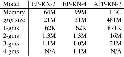
Table 1: Baseline and Comparison Models

4.1 Experimental set-up

All of our experiments use publically available re-sources. We use the French-English section of the Europarl(EP) corpus for parallel data and language modelling (Koehn, 2003) and the English Giga-word Corpus (LDC2003T05; GW) for additional language modelling.

Decoding is carried-out using the Moses decoder (Koehn and Hoang, 2007). We hold out 500 test sen-tences and 250 development sensen-tences from the par-allel text for evaluation purposes. The feature func-tions in our models are optimised using minimum error rate training and evaluation is performed using the BLEU score.

4.2 Baseline and comparison models

Our baseline LM and other comparison models are conventionaln-gram models smoothed using modi-fied Kneser-Ney and built using the SRILM Toolkit (Stolcke, 2002); as is standard practice these models drop entries forn-grams of size 3 and above when the corresponding discounted count is less than 1. The baseline language model, EP-KN-3, is a trigram model trained on the English portion of the parallel corpus. For additional comparisons we also trained a smoothed 4-gram model on this Europarl data (EP-KN-4) and a trigram model on the Agence France Press section of the Gigaword Corpus (AFP-KN-3). Table 1 shows the amount of memory these mod-els take up on disk and compressed using the gzip utility in parentheses as well as the number of dis-tinctn-grams of each order. We give the gzip com-pressed size as an optimistic lower bound on the size of any lossless representation of each model.2

2

Corpus Europarl Gigaword

1-gms 61K 281K

2-gms 1.3M 5.4M

3-gms 4.7M 275M

4-gms 9.0M 599M

5-gms 10.3M 842M 6-gms 10.7M 957M

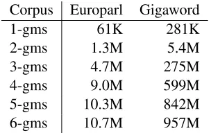
Table 2: Number of distinctn-grams

4.3 Bloom filter-based models

To create Bloom filter LMs we gathered n-gram counts from both the Europarl (EP) and the whole of the Gigaword Corpus (GW). Table 2 shows the numbers of distinctn-grams in these corpora. Note that we use no pruning for these models and that the numbers of distinctn-grams is of the same or-der as that of the recently released Google Ngrams dataset (LDC2006T13). In our experiments we cre-ate a range of models referred to by the corpus used (EP or GW), the order of then-gram(s) entered into the filter (1 to 10), whether the model is Boolean (Bool-BF) or provides frequency information (Freq-BF), whether or not sub-sequence filtering was used (FTR) and whether it was used in conjunction with the baseline trigram (+EP-KN-3).

4.4 Machine translation experiments

Our first set of experiments examines the relation-ship between memory allocated to the BF and BLEU score. We present results using the Boolean BF-LM in isolation and then both the Boolean and log-frequency BF-LMS to add 4-grams to our baseline 3-gram model.Our second set of experiments adds 3-grams and 5-grams from the Gigaword Corpus to our baseline. Here we constrast the Boolean BF-LM with the log-frequency BF-BF-LM with different quantisation bases (2 = fine-grained and 5 = coarse-grained). We then evaluate the sub-sequence fil-tering approach to reducing the actual error rate of these models by adding both 3 and 4-grams from the Gigaword Corpus to the baseline. Since the BF-LMs easily allow us to deploy very high-order n-gram models, we use them to evaluate the impact of dif-ferent ordern-grams on the translation process pre-senting results using the Boolean and log-frequency BF-LMin isolationforn-grams of order 1 to 10.

Model EP-KN-3 EP-KN-4 AFP-KN-3

BLEU 28.51 29.24 29.17

Memory 64M 99M 1.3G

gzipsize 21M 31M 481M

Table 3: Baseline and Comparison Models

4.5 Analysis of BF extensions

We analyse our log-frequency BF scheme in terms of the additional memory it requires and the error rate compared to a redundant scheme. The non-redundant scheme involves entering just the exact quantised count for eachn-gram and then searching over the range of possible counts at test time starting with the count with maximum a priori probability (i.e. 1) and incrementing until a count is found or the whole codebook has been searched (here the size is 16).

We also analyse the sub-sequence filtering scheme directly by creating a BF with only 3-grams and a BF containing both 2-grams and 3-grams and comparing their actual error rates when presented with 3-grams that are all known to be negatives.

5 Results

5.1 Machine translation experiments

Table 3 shows the results of the baseline (EP-KN-3) and other conventionaln-gram models trained on larger corpora (AFP-KN-3) and using higher-order dependencies (EP-KN-4). The larger models im-prove somewhat on the baseline performance.

Figure 1 shows the relationship between space al-located to the BF models and BLEU score (left) and false positive rate (right) respectively. These experi-ments donotinclude the baseline model. We can see a clear correlation between memory / false positive rate and translation performance.

Adding 4-grams in the form of a Boolean BF or a log-frequency BF (see Figure 2) improves on the 3-gram baseline with little additional memory (around 4MBs) while performing on a par with or above the Europarl 4-gram model with around 10MBs; this suggests that a lossy representation of the un-pruned set of 4-grams contains more useful informa-tion than a lossless representainforma-tion of the pruned set.3

3

29

28

27

26

25

10 8

6 4

2

1

0.8

0.6

0.4

0.2

0

BLEU Score

False positive rate

Memory in MB

Europarl Boolean BF 4-gram (alone)

BLEU Score Bool-BF-EP-4 False positive rate

Figure 1: Space/Error vs. BLEU Score.

30.5

30

29.5

29

28.5

28

9 7

5 3

1

BLEU Score

Memory in MB

EP-Bool-BF-4 and Freq-BF-4 (with EP-KN-3)

EP-Bool-BF-4 + EP-KN-3 EP-Freq-BF-4 + EP-KN-3 EP-KN-4 comparison (99M / 31M gzip) EP-KN-3 baseline (64M / 21M gzip)

Figure 2: Adding 4-grams with Bloom filters.

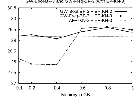
As the false positive rate exceeds 0.20 the perfor-mance is severly degraded. Adding 3-grams drawn from the whole of the Gigaword corpus rather than simply the Agence France Press section results in slightly improved performance with signficantly less memory than the AFP-KN-3 model (see Figure 3).

Figure 4 shows the results of adding 5-grams drawn from the Gigaword corpus to the baseline. It also contrasts the Boolean BF and the log-frequency BF suggesting in this case that the log-frequency BF can provide useful information when the quantisa-tion base is relatively fine-grained (base 2). The Boolean BF and the base 5 (coarse-grained quan-tisation) log-frequency BF perform approximately the same. The base 2 quantisation performs worse

30.5

30

29.5

29

28.5

28

27.5

27

1 0.8

0.6 0.4

0.2 0.1

BLEU Score

Memory in GB

GW-Bool-BF-3 and GW-Freq-BF-3 (with EP-KN-3)

GW-Bool-BF-3 + EP-KN-3 GW-Freq-BF-3 + EP-KN-3 AFP-KN-3 + EP-KN-3

Figure 3: Adding GW 3-grams with Bloom filters.

30.5

30

29.5

29

28.5

28

1 0.8

0.6 0.4

0.2 0.1

BLEU Score

Memory in GB

GW-Bool-BF-5 and GW-Freq-BF-5 (base 2 and 5) (with EP-KN-3)

GW-Bool-BF-5 + EP-KN-3 GW-Freq-BF-5 (base 2) + EP-KN-3 GW-Freq-BF-5 (base 5) + EP-KN-3 AFP-KN-3 + EP-KN-3

Figure 4: Comparison of different quantisation rates.

for smaller amounts of memory, possibly due to the larger set of events it is required to store.

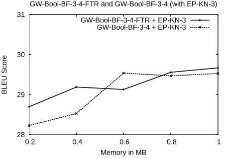
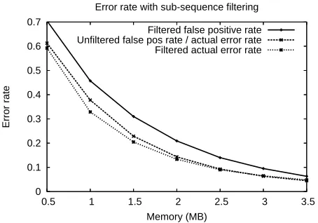
Figure 5 shows sub-sequence filtering resulting in a small increase in performance when false positive rates are high (i.e. less memory is allocated). We believe this to be the result of an increased a pri-ori membership probability for n-grams presented to the filter under the sub-sequence filtering scheme.

Figure 6 shows that for this task the most useful

n-gram sizes are between 3 and 6.

5.2 Analysis of BF extensions

31

30

29

28

1 0.8

0.6 0.4

0.2

BLEU Score

Memory in MB

GW-Bool-BF-3-4-FTR and GW-Bool-BF-3-4 (with EP-KN-3)

GW-Bool-BF-3-4-FTR + EP-KN-3 GW-Bool-BF-3-4 + EP-KN-3

Figure 5: Effect of sub-sequence filtering.

27

26

25

24

10 9 8 7 6 5 4 3 2 1

BLEU Score

N-gram order

EP-Bool-BF and EP-Freq-BF with different order N-grams (alone)

EP-Bool-BF EP-Freq-BF

Figure 6: Impact ofn-grams of different sizes.

BF for various order n-gram sets from the Giga-word Corpus with the same underlying false posi-tive rate (0.125). The additional space required by our scheme for storing frequency information is less than a factor of 2 compared to the standard BF.

Figure 7 shows the number and size of frequency estimation errors made by our log-frequency BF scheme and a non-redundant scheme that stores only the exact quantised count. We presented 500K nega-tives to the filter and recorded the frequency of over-estimation errors of each size. As shown in Section 3.1, the probability of overestimating an item’s fre-quency under the log-frefre-quency BF scheme decays exponentially in the size of this overestimation er-ror. Although the non-redundant scheme requires

0 10 20 30 40 50 60 70 80

16 15 14 13 12 11 10 9 8 7 6 5 4 3 2 1

Frequency (K)

Size of overestimation error Frequency Estimation Errors on 500K Negatives

Log-frequency BF (Bloom error = 0.159) Non-redundant scheme (Bloom error = 0.076)

Figure 7: Frequency estimation errors.

0 100 200 300 400 500 600 700

1 2 3 4 5 6 7

Memory (MB)

N-gram order (Gigaword)

Memory requirements for 0.125 false positive rate

Bool-BF Freq-BF (log base-2 quantisation)

Figure 8: Comparison of memory requirements.

fewer items be stored in the filter and, therefore, has a lower underlying false positive rate (0.076 versus 0.159), in practice it incurs amuchhigher error rate (0.717) with many large errors.

0 0.1 0.2 0.3 0.4 0.5 0.6 0.7

0.5 1 1.5 2 2.5 3 3.5

Error rate

Memory (MB)

Error rate with sub-sequence filtering

Filtered false positive rate Unfiltered false pos rate / actual error rate Filtered actual error rate

Figure 9: Error rate with sub-sequence filtering.

6 Related Work

We are not the first people to consider building very large scale LMs: Kumar et al. used a four-gram LM for re-ranking (Kumar et al., 2005) and in un-published work, Google used substantially largern -grams in their SMT system. Deploying such LMs requires either a cluster of machines (and the over-heads of remote procedure calls), per-sentence fil-tering (which again, is slow) and/or the use of some other lossy compression (Goodman and Gao, 2000). Our approach can complement all these techniques. Bloom filters have been widely used in database applications for reducing communications over-heads and were recently applied to encode word frequencies in information retrieval (Linari and Weikum, 2006) using a method that resembles the non-redundant scheme described above. Exten-sions of the BF to associate frequencies with items in the set have been proposed e.g., (Cormode and Muthukrishn, 2005); while these schemes are more general than ours, they incur greater space overheads for the distributions that we consider here.

7 Conclusions

We have shown that Bloom Filters can form the ba-sis for space-efficient language modelling in SMT. Extending the standard BF structure to encode cor-pus frequency information and developing a strat-egy for reducing the error rates of these models by sub-sequence filtering, our models enable

higher-ordern-grams and larger monolingual corpora to be used more easily for language modelling in SMT. In a companion paper (Talbot and Osborne, 2007) we have proposed a framework for deriving con-ventional smoothed n-gram models from the log-frequency BF scheme allowing us to do away en-tirely with the standard n-gram model in an SMT system. We hope the present work will help estab-lish the Bloom filter as a practical alternative to con-ventional associative data structures used in compu-tational linguistics. The framework presented here shows that with some consideration for its workings, the randomised nature of the Bloom filter need not be a significant impediment to is use in applications.

References

B. Bloom. 1970. Space/time tradeoffs in hash coding with allowable errors.CACM, 13:422–426.

A. Broder and M. Mitzenmacher. 2005. Network applications of bloom filters: A survey.Internet Mathematics, 1(4):485– 509.

David Chiang. 2005. A hierarchical phrase-based model for statistical machine translation. InProceedings of the 43rd Annual Meeting of the Association for Computational Lin-guistics (ACL’05), pages 263–270, Ann Arbor, Michigan. G. Cormode and S. Muthukrishn. 2005. An improved data

stream summary: the count-min sketch and its applications.

Journal of Algorithms, 55(1):58–75.

J. Goodman and J. Gao. 2000. Language model size reduction by pruning and clustering. InICSLP’00, Beijing, China. Philipp Koehn and Hieu Hoang. 2007. Factored translation

models. InProc. of the 2007 Conference on Empirical Meth-ods in Natural Language Processing (EMNLP/Co-NLL). P. Koehn. 2003. Europarl: A multilingual corpus for

eval-uation of machine translation philipp koehn, draft. Available at:http://people.csail.mit.edu/ koehn/publications/europarl.ps. S. Kumar, Y. Deng, and W. Byrne. 2005. Johns Hopkins

Uni-versity - Cambridge UniUni-versity Chinese-English and Arabic-English 2005 NIST MT Evaluation Systems. InProceedings of 2005 NIST MT Workshop, June.

Alessandro Linari and Gerhard Weikum. 2006. Efficient peer-to-peer semantic overlay networks based on statistical lan-guage models. InProceedings of the International Workshop on IR in Peer-to-Peer Networks, pages 9–16, Arlington. Andreas Stolcke. 2002. SRILM – An extensible language

mod-eling toolkit. In Proc. of the Intl. Conf. on Spoken Lang. Processing, 2002.