Cointegration Based Regression to Analyse Linkage between Share Price Index and Macroeconomic Variables: Evidence from Colombo Stock Exchange

ISSN Online: 2333-9721 ISSN Print: 2333-9705

Cointegration Based Regression to Analyse

Linkage between Share Price Index and

Macroeconomic Variables: Evidence from

Colombo Stock Exchange

Gayani Thalagoda, Kusal Rathnayake, Sachith Abeysundara

Department of Statistics and Computer Science, University of Peradeniya, Peradeniya, Sri Lanka

Abstract

The main objective of the study is to investigate the long run performance of the All Share Price Index (ASPI) of the Colombo Stock Exchange, based on the economic activities of Sri Lanka using cointegration and auto regressive time series. The cointegration test illustrates that share price index is cointe-grated with a specific set of macroeconomic variables, i.e. exchange rate (USD/LKR), money supply, wage rates, wet foreign assets, currency in circu-lation, imports and exports with 95% confidence. The study also proposes a regression model using Eigen Vector coefficients to predict the behavior of ASPI index in the long run. The model performance, evaluated using the re-siduals of the test data, represents a random behavior indicating a valid long-run cointegration regression relationship between ASPI and other mac-roeconomic variables. Future studies involve analysis of the short-run rela-tionship among the macroeconomic variables using Vector Error Correlation Model.

Subject Areas

Applied Statistical Mathematics, Case Studies and Management Information Systems, Financial Mathematics, Monetary Economics,

Statistics and Econometrics

Keywords

Cointegration, Stationarity, Time Series, Regression, Unit Root Tests

1. Introduction

Studying the stock market performance of a country, for long, has been

consid-How to cite this paper: Thalagoda, G., Rathnayake, K. and Abeysundara, S. (2018) Cointegration Based Regression to Analyse Linkage between Share Price Index and Macroeconomic Variables: Evidence from Colombo Stock Exchange. Open Access Library Journal, 5: e4955.

https://doi.org/10.4236/oalib.1104955

Received: October 2, 2018 Accepted: November 27, 2018 Published: November 30, 2018

Copyright © 2018 by authors and Open Access Library Inc.

This work is licensed under the Creative Commons Attribution International License (CC BY 4.0).

http://creativecommons.org/licenses/by/4.0/

Open Access

ered as an effective alternative for realizing quick profits. The stock market is the market where common stocks representing ownership in a company are traded

[1]. One of the major reasons to invest in a stock market is the substantially high growth potential it offers when compared to other investment options. It plays an important role in national economies, as they are considered to be very help-ful in channelling and diversifying the domestic savings and foreign capital into productive investment, fostering capital formation and sustaining economic growth and development [2].

Government financial policies and other macroeconomic fluctuations are be-lieved to have a consequential influence on the activities of the stock market. Many macroeconomic variables such as, inflation rate, exchange rate, money supply and gross domestic production is said to have an impact in the share market performance of a country.

This study examines the role of macroeconomic variables on stock prices movement in Sri Lanka. It investigates the dynamic interactions between fifteen macroeconomic variables and the stock prices i.e. ASPI index, for an emerging market, Sri Lanka, using co-integration and Granger causality tests.

The main objective of the study is to predict the performance of the Colombo Stock Exchange, All Share Price Index, based on the other macroeconomic vari-ables in the study under concern. Initially, we aim to recognize whether there exists a relationship between ASPI and other macroeconomic variables and thereby to analyse the nature of the relationship the variables carry.

We also aim to develop a regression model through co-integration technique to predict the behavior of ASPI index in the long run and a VECM (Vector error correction model) to predict the behavior of ASPI in the short run.

Colombo Stock Exchange (CSE) remained underdeveloped during the pre-war period due to unstable political and economic conditions. CSE reported a robust growth in the post-war period due to noteworthy economic growth and peaceful political environment. However, despite the impressive economic envi-ronment emerged, the stock market growth was not sustained after 2012. Thus, the constraints for stock market development remain unclear [3].

The Colombo Stock Exchange is the main stock exchange in Sri Lanka. It pro-vides a fully automated platform for the investors. The Colombo Stock Exchange (CSE) has 296 companies representing 20 business sectors as at 3 August 2015, with a Market Capitalization of Rs. 3115.52 Bn. Even though there are two share price indices active in CSE, namely, ASPI and S&P Sri Lanka price index, our consideration rests on the prediction of ASPI.

If a time series model is stationary, it is believed that the estimated values will have an economic meaning. For non-stationary time series spurious results will be obtained [4]. Co-integration can be applied only if the variables under con-cern are stationary in the same difference level, either I(0) or I(1).

Efficient market theory, based on the randomness of the market, explains that the market cannot be beaten due to its highly dynamic behavior. Further, EMH

states that it is impossible to gain massive profits through buying undervalued stocks and selling them later for an over price, because that involves prediction.

All in all, the theory states that, in an efficient market, the only way to obtain higher profits is by engaging in riskier profits and not exploiting undervalued stocks. This fair-game reason has been a huge motivator for many investors to actively participate in the stock market. Thus, study the stock market.

2. Previous Studies

The stock market is the market where common stock representing ownership in a company, are traded [1]. The previous studies show that the most important macroeconomic variables are Gross domestic product (GDP), inflation, money supply, interest rate, exchange rate, unemployment rate, foreign direct invest-ment and index of industrial production [5]. Menike in 2006 [6], writes that stock market is the leading indicator of an economy reflect the level of economic activities in the country. She used Multiple Regression models to examine the effect of macroeconomic variables on stock prices in selected companies in the CSE inflation rate and exchange rate react mainly negatively to stock prices in the Colombo Stock Exchange (CSE). It was found that lagged money supply variables were insignificant.

Even though there have been many studies have been investigated the rela-tionship between macroeconomic variables and stock market returns in devel-oped countries. Solnik in 1987, [7] examined the impact of several variables (exchange rates, interest rates and changes in inflationary expectation) on stock prices. He uses monthly data from nine western markets (U.S., Japan, Germany, U.K., France, Canada, Netherlands, Switzerland, and Belgium). He found depre-ciation to have a positive but insignificant influence on the U.S. stock market compared to change in inflationary expectation and interest rates.

Hosseini in 2011, [8], investigated relationship between stock market indices and macroeconomic variables namely crude oil price (COP), money supply (M2), industrial production (IP) and inflation rate (IR) in China and India. They used Johansen Co-integration technique for long run equilibrium assessment and VECM technique for short-term structural equilibrium assessment. The pa-per concludes that there exist both short run and long run linkages between macroeconomic variables and stock market index in each of these two countries.

Mohammad et al. in 2009 [9], explored the correlation among the macroeco-nomic variables and share price of KSE (Karachi Stock Exchange).

However, it is obvious that there is a shortage of literature concerning on emerging stock markets, especially Sri Lankan stock market. Samarakoon in 1996, [10] in his works, reported a positive relationship between stock market returns and inflation. Based on the best of knowledge from our of the reviewed literature, only Ratnayake in 2014, [11] has attempted to examine the impact of macroeconomic variables such as interest rate, inflation rate, exchange rate, money supply on stock market returns using cointegration for the Sri Lankan

Stock Exchange (CSE).

3. Research Methodology

3.1. Data Collection

The data used to carry out the analysis spans from 1st _{of January 2002 to 1}st _of

December 2016. There are 186 observations taken on a monthly basis. All Share Price Index (ASPI) value was used to reflect the Share prices in Sri Lanka [4] [12]. Further, the analysis comprises of total 15 macroeconomic variables re-flecting the economic condition of the major sectors of Sri Lanka.

We consider, All Share Price Index, Exchange Rate (USD/LKR), Interest Rate, Inflation rate, M1, M2, M4, Wage Rate of Government sector, Wage Rate of Trades, Net Foreign Assets, Currency in Circulation, Imports from all countries to Sri Lanka and Exports from Sri Lanka to all other countries as the variables under study.

The training set comprises of 144 observations spanning form January 2002 to December 2013. The test set comprises of 12 observations spanning from Janu-ary 2014 to December 2014.

3.2. Theory

At the most initial stage, a basic descriptive analysis is carried out to have a comprehensive idea about the variables under study. Since the variables are in different ranges, we consider the log transformation of variables in order to avoid heteroskedascity, the systemic damage to the distribution of residuals. This homoskedascity eventually helps in obtaining a more efficient analysis.

Next, simple correlation analysis is carried out to observe the relationship between pairs of variables and there by recognize which variables could be ade-quately correlated.

Prior to time series analysis, we conduct tests for normality of the variables, in order to see whether any of the variables we consider relates to a normal distri-bution. Under normality check, Jarque-Bera test checks whether the data from variables follow a normal distribution.

Thereafter, we conduct the graphical analysis. We plot time series of each variable to inspect if the data points are random or exhibit any pattern. Auto correlations plots and partial auto correlation plots obtained provide a prelimi-nary idea about the stationarity of the time series variables at hand.

Once the graphical analysis is completed, next step is to obtain a quantitative measurement for the stationarity of the time series. We carry out a formal inves-tigation by examining the stochastic properties of the variables.

Unit Root Tests which are employed to test the stationarity of the variables are crucial for analyzing the order of integration of the variable, thus, for carrying out cointegraion. Unit root tests are usually performed on each of the variables to determine the order of integration of these series. Under our study, we take use of Augmented Dickey Fuller Test (ADF) and Philips Peron Test (PP) [13].

Basic Dickey Fuller, the most common test, for testing first order integration

i.e. I(0)versus zeroth order i.e. I(0) integration checks the hypothesis of, a vari-able having a unit root. However, it covers only a special case of time series, Auto Regressive Time Series. Augmented Dickey Fuller Test (ADF) is more powerful, thus, can be applied when the error terms (ut) (2) are correlated. We

choose a lag length to so that the residuals aren’t serially correlated to overcome the auto correlation effect. We either minimize Akaike’s information criterion (AIC) or Bayesian information criterion (BIC). Phillips-Perron Test is the other unit root we conduct under our study. The test uses a null hypothesis that a given time series is of order 1 i.e.I(1). Under the study in concern, we discuss both Augmented Dickey Fuller (ADF) test and also Phillips-Peron (PP) test.

The difference between the two tests is in their approach to addressing the is-sue of data series possibly carrying a higher order or auto correlation that what is admitted in the equation.

Auto Regressive equation:

1

t t t

y α βt γy₋ u

∆ = + + + ₍₁₎

Augmented Dickey Fuller Equation:

1 1 1 1

t t t p t p t

y α βt γy− δ y− δ − y− u

∆ = + + + ∆ ++ ∆ + (2)

Here yt denotes the value of time series variable at a given time period t, α

denotes a constant,

β

t

u is the error component of the model at t. The ADF test addresses the issue or serial correlation by introducing the lags of the first differences

(

)

Phillips-Perron test makes a non-parametric correction to the t-test statistic to account for serial correlation. Thus, PP test is more robust due to unspecified auto correlation and heteroskedasticity in the error term. However, PP test is less powerful than ADF test.

Once we classify variables as I(0), I(1) or of other integrated high order, we begin cointegration procedure. Co-integration is a statistical technique, which makes it possible to set up models that lead to stationary relations among va-riables where standard inference is possible. In a multivariate time series setting, it is often of interest whether two or more series are cointegrated and of which rank. If data from a linear combination of two or more variables can be statio-nary i.e.I(0), despite those variables being individually non-stationary.

3.2.2. Johansen Test for Cointegration

Under out study, we focus on the Maximum Eigen Value technique under Jo-hansen Test. JoJo-hansen Eigen Test found by JoJo-hansen (1991) carries the most de-sirable statistical properties for checking cointegration in multivariate time se-ries. The null hypothesis is of having at most r cointegration relationships while alternate hypothesis is of having more than r relationships. Tsay in 2005, [14]

shows that the critical values of the test are found through simulation makes the test vulnerable to asymptotic properties. This makes the test sensitive to specifi-cations in small samples.

Initially, maximum Eigen value technique under Johansen Co-integration method is carried out. Meanwhile the Maximum Eigenvalue test is formulated as:

(

)

(

)

max r r, 1 TIn 1 ˆr 1

λ + = − −λ+ (3)

r = Number of cointegrating vectors under the null hypothesis.

λ

Once the set of Eigen Values are calculated, we pull the maximum Eigen Val-ue. We then pull the number of cointegrating vectors. The null hypothesis is that the existence of r cointegrating vector and the alternative hypothesis is (r + 1) cointegrating vectors. Thereafter, we obtain the co-integration relation using the results we pulled in previous steps.

3.2.3. Hypothesis

If the cointegration analysis indicates that there is a cointegrating vector, we in-fer that the tested series will not drift apart in the long-term, and will revert to equilibrium levels following any short-term drift that may take place [15].

Once we obtain a co-integration relationship among the time series under consideration, we check for the stationarity of the residuals of the obtained model. Similar to the previous case, we use ADF test to check the stationarity of the residual time series. Provided the residual time series fulfils the stationarity condition, we establish the cointegrated regression model for the impact of ma-croeconomic variables on ASPI index for the long run.

We use the test data set, which, we prepared at the beginning of the study to validate the model we secure.

Given there exists at least one log run co-integrating relationship among the macroeconomic variables, the causal relationship among these variables can be determined by estimating the Vector Error Correlation Model. We utilize Gran-ger Causality Tests and Vector Error Correction Method in Time Series analysis to examine the short run relationship among the variables.

3.3. Research Methodology

Table 1 provides a description of variables, which will be investigated under the study.

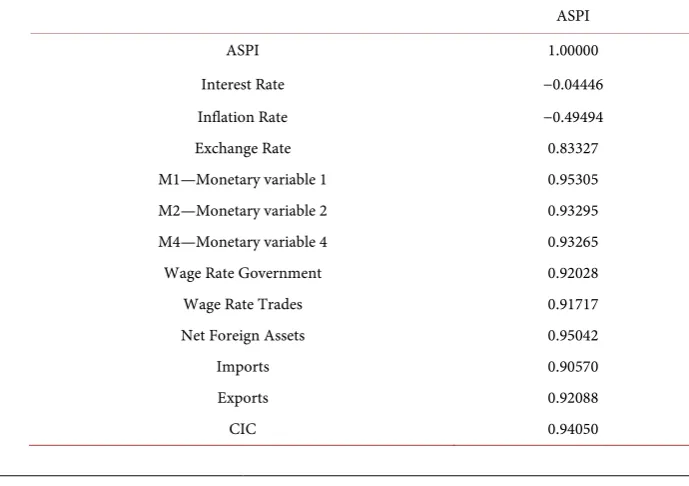
Table 2 demonstrates that although Inflation rates and interest rates are con-sidered as main branches of economy, they do not show significant correlation with ASPI. These results match with findings of Sohail and Zakir in 2011 [16]. Interest rate has the least interrelationship with the ASPI values with only −0.04446355. Thus, we no longer consider Interest rate as an explanatory vari-able for predicting ASPI values. Jarque-Bera test for each varivari-able rejects null hypothesis of a normal distribution at 5% significance level.

Table 1. Variable description of macroeconomic variables under the study.

Variable

Code Variable Name

ASPI All share price Index; the principal stock exchange of Colombo Stock Exchange Exchange

Rate Exchange Rate of US Dollar ($) to Sri Lankan Rupee (LKR) Interest Rate Amount of money due per a period as a ratio of the amount lent

Inflation Rate _{rising and the rate at which the purchasing power of money falls.} Rate at which the general level of prices for goods and services is

M1 The money supply that includes physical currency and coin, demand deposits, _{traveller’s checks, other checkable deposits. 24-hour money market funds}

M2 The money which refers to savings deposits, money market securities, mutual _{funds and other time deposits. Money market funds for more than 24 hours}

M4 A measure of broad money

Wage Rate

Trade Amount of base wage paid to a worker per unit of time (as per hour or day) or per unit of output if on piecework in the trade sector

Wage Rate

Government Amount of base wage paid to a worker per unit of time (as per hour or day) or per unit of output if on piecework in the government sector

Net Foreign Assets

The value of overseas assets owned by a nation, minus the value of its domestic assets that are owned by foreigners, adjusted for

changes in valuation and exchange rates. Currency in

Circulation The amount of individual units of a currency continued to be used for transactions

Imports The value of goods or services brought in to the home country _{form other countries}

Exports The value of goods or services sold out to other countries _{by one’s home country}

Table 2. Pair-wise correlations with ASPI.

ASPI

ASPI 1.00000

Interest Rate −0.04446

Inflation Rate −0.49494

Exchange Rate 0.83327

M1—Monetary variable 1 0.95305

M2—Monetary variable 2 0.93295

M4—Monetary variable 4 0.93265

Wage Rate Government 0.92028

Wage Rate Trades 0.91717

Net Foreign Assets 0.95042

Imports 0.90570

Exports 0.92088

CIC 0.94050

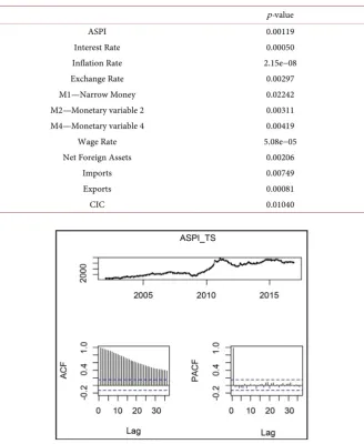
Table 3 demonstrates that none of the variables under concern follow a nor-mal distribution. Shapiro-Wilk Test, Jarque-Bera test, and QQ plots, they all sig-nified the non-normality nature of the data set under concern.

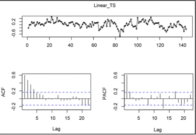
Graphical representation of time series of all variables indicated that all the variables were non-stationary in their natural form. The time series plots, along with their Auto-Correlation Function plots and Partial Auto-Correlation Func-tion plots clearly depicted the non staFunc-tionarity nature of the data. A trend com-ponent was visible for all the variables plotted.

Figure 1 shows the time series, Auto Correlated Function (ACF) and Partial

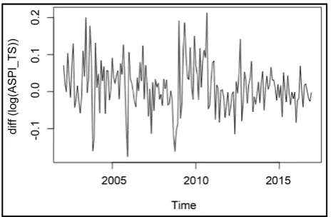
Auto Correlated Function (ACF) respectively. Since the trend component clearly depicted a I(0) nature time series, we move on to first order difference of the time series. Log differenced time series of each variable indicates a stationary behaviour. Figure 2 shows the time series of Log Differenced time series of ASPI index.

Table 3. Jarque Bera test for normality at 5% significance level.

p-value

ASPI 0.00119

Interest Rate 0.00050

Inflation Rate 2.15e−08

Exchange Rate 0.00297

M1—Narrow Money 0.02242

M2—Monetary variable 2 0.00311

M4—Monetary variable 4 0.00419

Wage Rate 5.08e−05

Net Foreign Assets 0.00206

Imports 0.00749

Exports 0.00081

CIC 0.01040

Figure 1. Time series, ACF and PACF of ASPI.

Figure 2. Time series of log differenced ASPI.

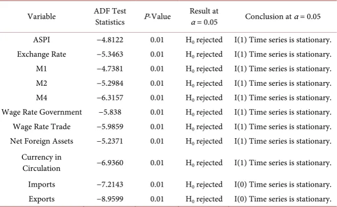
Table 4 demonstrates the ADF test results of the macroeconomic variables

selected after initial correlation analysis.

ADF Test statistics at 5% significance level is −2.89 for the standard model of no time trend component. ADF Test at 5% significance level showed that all the variables, in their log-differenced form are stationary time series. Phillips Peron Test too indicates that all macroeconomic variables in their log-differenced form, are I(1), stationary series at 5% significance level. By combining results of both ADF test and Phillips Peron test, all the variables except Interest Rate and Inflation rate are selected for the next level of the analysis.

The best Auto Regressive Model for the data under consideration suggests a lag length of 10. Considering the following criteria; Akaike’s Information crite-rion, Hannan-Quizz criterian, Schwarz criterian and Final Prediction Error cri-terian chooses the lag length.

Johansen Cointegration Test calculates the number of cointegration relations for multivariate time series. Table 5 demonstrates the results of Johansen Coin-tegration Test.

Johansen Cointegration test fails to reject the null hypothesis when r ≤ 11. Thus, result of the test is that there are eleven cointegration relations. Next, we find out the set of cointegration relations which correspond to the maximum Eigen Value. Maximum Eigen Value Technique under Johansen Cointegration procedure gives several λ Eigen values. Maximal eigenvalue statistic (lambda max), without linear trend and constant in cointegration is 0.87521.

The set of cointegration relations corresponding to the maximum Eigen value is shown below. Thereafter, we obtain our Regression model based on the coin-tegration relations. Table 6 demonstrates the cointegration relationships.

Linear combination of 11 time series with the coefficient values obtained from the Johansen co-integration test results are as then subjected to the ADF test to check stationarity of the residuals with 5% significance level. It shows The

p-value of the test is 0.03739. Thus, we can say that there is enough evidence to state that the linearly combined time series is stationary, I(0) under 5% signifi-cance level.

Table 4. Augmented dickey-fuller test results.

Variable ADF Test _Statistics P-Value Result at _{α = 0.05} Conclusion at α = 0.05

ASPI −4.8122 0.01 H0 rejected I(1) Time series is stationary.

Exchange Rate −5.3463 0.01 H0 rejected I(1) Time series is stationary.

M1 −4.7381 0.01 H0 rejected I(1) Time series is stationary.

M2 −5.2984 0.01 H0 rejected I(1) Time series is stationary.

M4 −6.3157 0.01 H0 rejected I(1) Time series is stationary.

Wage Rate Government −5.838 0.01 H0 rejected I(1) Time series is stationary.

Wage Rate Trade −5.9859 0.01 H0 rejected I(1) Time series is stationary.

Net Foreign Assets −5.2371 0.01 H0 rejected I(1) Time series is stationary.

Currency in

Circulation −6.9360 0.01 H0 rejected I(1) Time series is stationary.

Imports −7.2143 0.01 H0 rejected I(0) Time series is stationary.

Exports −8.9599 0.01 H0 rejected I(0) Time series is stationary.

Table 5. Johansen test results for number of cointegration relations.

At most i (r ≤ i) Test Statistic Critical Value at 5% _significance Conclusion

At most 10 23.93 9.24 H0 rejected.

At most 9 34.49 15.67 H0 rejected.

At most 8 38.58 22.00 H0 rejected.

At most 7 60.13 28.14 H0 rejected.

At most 6 68.13 34.40 H0 rejected.

At most 5 113.95 40.30 H0 rejected.

At most 4 125.15 46.45 H0 rejected.

At most 3 165.73 52.00 H0 rejected.

At most 2 179.46 57.42 H0 rejected.

At most 1 217.37 63.57 H0 rejected.

At most 0 278.88 69.74 H0 rejected.

Table 6. Cointegration relations of the multivariate time series.

Variable Indicating Cointegration Cointegration Value

ASPI 1.00000

Exchange Rate −2.67693

M1 −6.06898

M2 −5.02216

M4 6.65609

Wage Rate Government −0.01002

Wage Rate Trades −0.42577

Net Foreign Assets 0.25376

Currency In Circulation −3.65640

Imports −0.14862

Exports −0.49051

Constant 18.20775

Figure 3, which illustrates the cointegrated time series, shows promising re-sults. Next we conduct the Augmented Dickey Fuller test to obtain a quantitative measure to further ensure the cointegrated time series is stationary.

ADF test conducted rejects the null hypothesis of non-stationarity. P-value is 0.03739. Thus, we can say that there is enough evidence to state that the linearly combined time series is stationary, I(0) under 5% significance level.

Regression model using the results obtained previously is given below.

ASPI 2.67693 Exchange Rate 6.06898 M1 5.02216 M2 6.65609 M4 0.01002 Wage rate Government

0.42577 Wage Rate Trades 0.25376 Net Foreign Assets 3.65640 Currency In Circulation 0.14862 Imports 0.49051 Exp

= ∗ − ∗ + ∗

− ∗ + ∗

+ ∗ − ∗

− ∗ + ∗

+ ∗ orts 18.20775004+

(4)

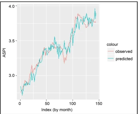
Figure 4 shows the predicted values versus the observed values.

4. Model Validation

Next we validate our regression model with the test data set. The validation pro-cedure provides promising results. Regression model is applied to the test set comprising of observations spanning from January 2014 to December 2014.

Figure 5 shows the residual time series. It depicts a random behaviour

indicat-ing a stationary time series.

Augmented Dickey Fuller Test further confirms Stationary behaviour of the residual time series (P-value = 0.02747). The test rejects the null hypothesis at 5% significance level. Thus we can conclude the residual time series is stationary at 5% significance level. Therefore the results of the study provide promising sults to state with 95% confidence that there exists a long-run cointegration re-gression relationship between ASPI and other macroeconomic variables.

Figure 3. Cointegrated time series.

Figure 4. Predicted values using the model versus actual values.

Figure 5. Time series of residuals.

Table 7 demonstrates the model validation measures, such as Mean Absolute

Percentage Error (MAPE) and Root Mean Square Error (RMSE), and these measures also confirm the validity of the model.

5. Conclusion

The study presents some interesting findings about the stock market of Sri Lanka. All Share Price Index of Colombo Stock Exchange has shown an im-provement throughout the period of time. Contrary to popular belief, the study clearly shows that there is no significant impact from Interest rate and Inflation Rate on the ASPI values under 5% significance level. The study also shows that

Table 7. Accuracy measure for model validity.

Accuracy Measure Value

RMSE Value 0.08055

MAPE Value 0.00860

real economic variables such as Imports, Exports, Wage Rates and money vari-ables have a significant co-movement with the ASPI in the long run. Johansen Test provides 11 cointegration relations and the linear regression model pre-sented using findings of the Johansen Test shows promising R-squared value of 0.9142668. Model validation using test data affirms that ASPI can be predicted using the leading indicators Exchange Rate (USD/LKR), M1, M2, M4, Wage Rate of Government sector, Wage Rate of Trades, Net Foreign Assets, Currency in Circulation, Imports from all countries to Sri Lanka and Exports from Sri Lanka to all other countries.

6. Discussion

Following our study, there are many factors we consider when we arrive at con-clusion. In general, we discuss limitations of our study under this section. We consider data from the secondary sources i.e. published reports from Colombo Stock Exchange. To allow a more complete picture of the co-movement patterns it could be advantageous to include data of higher frequency i.e. hourly data or daily data rather than monthly data used in this study.

Even though there are two major indices of Colombo Stock market perform-ance, we use only the more prominent one of the two indices, the ASPI. Future studies may incorporate the remaining index too, in order to gain a more holis-tic view of the impact.

In our study we use Johansen Test over Engle-Grangers Two Step Model due to two main reasons. Even though two-step model is comparatively easy to run, it requires a larger sample size to avoid plausible error. Moreover, it can only be run over two variables at most [17]. Further, hypothesis testing on existence of cointegrating relationships themselves is impossible [17]. Since our study envi-ronment is multivariate we adapt to Johansen Test over Engle Grange Two Step model.

We use both ADF test and PP test to overcome each other test’s conditional faults. Even though ADF is the more powerful of the two tests, it loses its power when the lag length is a sufficiently large value.

During our model evaluation using test data, we take in to account MAPE value, RMSE value and MSE value. We do no consider the R-squared value, since it is not appropriate in evaluating the regression model for test data. How-ever, when R-squared value is tested upon the train data, it provides promising results.

Under the study, we have considered only the long run co-movement impact of macroeconomic variables on the All Share Price Index of Colombo Stock

Exchange. In our future studies we hope to study the short run co-movement and stochastic trends between ASPI and other macroeconomic variables.

Conflicts of Interest

The authors declare no conflicts of interest regarding the publication of this pa-per.

References

[1] Mishkin, F.S. and Eakins, S.G. (2011) Financial Markets and Institutions. 4th Edi-tion, Pearson Series in Finance.

[2] Kalyanaraman, L. and Tuwajri, B.A. (2014) Macroeconomic Forces and Stock Prices: Some Empirical Evidence from Saudi Arabia. International Journal of Fi-nancial Research, 5, No. 1; 2014.

[3] Kulathunga, K.M.M.C.B. (2015) Macroeconomic Factors and Stock Market Devel-opment: With Special Reference to Colombo Stock Exchange. International Journal of Scientific and Research Publications (IJSRP), 5, Issue 8.

http://www.ijsrp.org/research-paper-0815.php?rp=P444412

[4] Çağlı, E., Taşkın, D. and Halaç, U. (2010) Testing Long-Run Relationship between Stock Market and Macroeconomic Variables in the Presence of Structural Breaks: The Turkish Case. International Research Journal of Finance and Economics, 48, 49-60.

[5] Alam, Z. and Rashid, K. (2014) Time Series Analysis of the Relationship between Macroeconomic Factors and the Stock Market Returns in Pakistan. Journal of Yasar University, 9, 6261-6380.

[6] Menike, L. (2010) The Effect of Macroeconomic Variables on Stock Prices in Emerging Sri Lankan Stock Market. Sabaragamuwa University Journal, 6, 50-67.

https://doi.org/10.4038/suslj.v6i1.1689

[7] Solnik, B. (1987) Using Financial Prices to Test Exchange Rate Models: A Note. The Journal of Finance, 42, 141-149. https://doi.org/10.1111/j.1540-6261.1987.tb02555.x

[8] Hosseini, S.M. (2011) The Role of Macroeconomic Variables on Stock Market Index in China and India. International Journal of Economics and Finance, 3, 233-243. [9] Jalil, M.A., Mohammad, S. and Hussain, A. (2009) Impact of Macroeconomics

Variables on Stock Prices: Empirical Evidence in Case of KSE. European Journal of Scientific Research, 38, No. 1. https://doi.org/10.2139/ssrn.1683357

[10] Samarakoon, L.P. (1996) Stock Market Returns and Inflation: Sri Lankan Evidence (October 1996). Sri Lankan Journal of Management, 1, 293-311.

[11] Ratnayake, R.M.I.P, WIjekoon, P. and Yapa, D. (2014) Relationship between All Share Price Index (ASPI) and Macroeconomic Variables: Evidence from Sri Lanka,

International Journal of Development Research, 4, 1923-1928.

[12] Rahman, M.L. and Uddin, J. (2009) Dynamic Relationship between Stock Prices and Exchange Rates: Evidence from Three South Asian Countries. International Busi-ness Research, 2, 167.

[13] Dickey, D. and Fuller, W. (1981) Likelihood Ratio Statistics for Autoregressive Time Series with a Unit Root. Econometrica, 49, 1057-1072.

https://doi.org/10.2307/1912517

[14] Tsay, R.S. (2005) Analysis of Financial Time Series. 2nd Edition, Wiley-Interscience.

https://doi.org/10.1002/0471746193

[15] Maggiora, D. and Skerman, R. (2009) Johansen Cointegration Analysis of American and European Stock Market Indices: An Empirical Study. Lund University, Lund. [16] Sohail, N. and Hussain, Z. (2011) The Macroeconomic Variables and Stock Returns

in Pakistan: The Case of KSE 100 Index. International Research Journal of Finance and Economics, 80, 66-74.

[17] Brooks, C. (2008) RATS Handbook to Accompany Introductory Econometrics for Finance. Cambridge Books, Cambridge University Press.