An adaptive weighting based on modified DOP for
1collaborative indoor positioning
2Hao Jing1, James Pinchin2, Chris Hill1 and Terry Moore1 3
1(Nottingham Geospatial Institute, University of Nottingham, United Kingdom) 4
2(Horizon Digital Economy Research, University of Nottingham, United Kingdom) (E-mail: 5
ABSTRACT: 7
Indoor localisation has always been a challenging problem due to poor Global Navigation 8
Satellite System (GNSS) availability in such environments. While inertial measurement 9
sensors have become popular solutions to indoor positioning, it suffers large drifts after 10
initialisation. Collaborative positioning enhances positioning robustness by integrating 11
multiple localisation information, especially relative ranging measurements between local 12
users and transmitters. However, not all ranging measurements are useful throughout the 13
whole positioning process and integrating too much data will increase the computation cost. 14
To enable a more reliable positioning system, an adaptive collaborative positioning algorithm 15
is proposed which selects units for the collaborative network and integrates ranging 16
measurement to constrain inertial measurement errors. The algorithm selects the network 17
adaptively from three perspectives: the network geometry, the network size and the accuracy 18
level of the ranging measurements between the units. The collaborative relative constraint is 19
then defined according to the selected network geometry and anticipated measurement 20
quality. In the case of trials with real data, the positioning accuracy is improved by 60% by 21
adjusting the range constraint adaptively according to the selected network situation, while 22
also improving the system robustness. 23
1 INTRODUCTION 24
Location-based Services (LBS) have gradually expanded from military and government 25
departments into our everyday life. From emergency responders to social networks, LBS 26
users inevitably demand for more accurate and reliable positioning information in a wider 27
range of areas. Although Global Navigation Satellite Systems (GNSS) can provide accurate 28
positioning outdoors, but lacks the same accuracy and robustness in more complicated 29
environments due to signal disruption and blockage, e.g. inside buildings and urban canyons 30
(von Watzdorf, 2010). 31
Inertial navigation is a common approach in GNSS-denied environments, as it does not rely 32
on any infrastructure other than an inertial measurement unit (IMU) that works in almost any 33
environment. However they are notorious for gyro heading drifts, which could accumulate up 34
to tens of metres after just a few seconds. Therefore either corrections or external 35
measurements must be applied to inertial measurements to provide more reliable results 36
(Abdulrahim et al., 2011). Various inertial navigation system (INS) integration methods, such 37
as INS/GPS and INS/Wi-Fi integration, have been proposed where each sensor complement 38
the other if one fails during a short period (Evennou and Marx, 2006; Weyn and Schrooyen, 39
2008). Wireless signals are available indoors and naturally become a good alternative 40
indoors, even though it suffers signal instability (Narzullaev et al., 2008; Kaemarungsi and 41
Krishnamurthy, 2012). 42
introduced in intelligent transport systems. Roadside beacons and vehicle clusters helped to 44
maintain reliable positioning by correcting GNSS observations and reduce errors through 45
vehicle-to-vehicle ranging when the vehicle could not receive sufficient satellite signals (Yao 46
et al., 2011; Tang et al., 2012). For a more general idea of collaborative positioning, signal of 47
opportunities was introduced in (Yang et al., 2009) where positioning is achieved from 48
integrating a number of different types of signals in the surrounding environment. However, 49
the overall performance can be affected by the reliability of each particular signal, the amount 50
of data and the relative position. 51
This paper proposes a collaborative positioning solution for an indoor pedestrian navigation 52
scenario, which integrates measurements from multi-users through peer-to-peer (P2P) 53
ranging. Based on the signal properties in the indoor environment, this paper provides a 54
detailed analysis on the collaborative network structure and its effects on the positioning 55
result. A particle filter based adaptive ranging constraint collaborative positioning (ARCP) 56
algorithm is proposed which integrates inertial measurements, map information and relative 57
ranging. It improves the positioning accuracy and robustness in complicated indoor 58
environments by applying a selecting and weighting scheme to the ranging constraint on each 59
user based on the obtained ranging measurements and network geometry. Simulations are 60
carried out to analyse the network characteristics and the anticipated positioning outcome. 61
Finally, trials are carried out to validate the positioning algorithm performance. 62
2 SELECTING THE NETWORK 63
Multi-users can share local environment information and constrain errors directly through 64
P2P ranging between users (Jing et al., 2013). P2P ranging are relative ranging measurements 65
between nearby units, which can update and correct the user state model by restricting valid 66
measurements to the measured distance and pushing the final solution towards the true 67
position. Therefore, the ranging constraint plays a crucial role on the positioning 68
performance. To integrate only the most effective ranges, a decision-making scheme is 69
introduced here to enhance positioning accuracy and system efficiency. 70
The decision is made each epoch based on the current situation, hence is adaptable to 71
different measurement error models and network geometry. Three different aspects are 72
considered. First of all, the ranging measurement accuracy level estimated from signal 73
characteristics. Secondly, the network geometry of the collaborative network formed by 74
selected nodes. Finally, the network size should also be considered for efficiency. 75
The collaborative network discussed here consists of two types of units, fixed transmitters 76
with known positions, known as anchors (denoted as Tx), and mobile users whose positions 77
need to be determined, known as rovers (denoted as Rx). The optimal network should consist 78
the minimum number of units that produces the required positioning accuracy. The Cramer-79
Rao Lower Bound (CRLB) of different networks is presented below to examine the 80
relationship between network size, geometry and positioning accuracy. 81
2.1 Network Cramer-Rao Lower Bound 82
CRLB provides a lower boundary on the achievable variance of any unbiased location 83
estimator for unknown parameters, which is useful for justifying how well an estimator can 84
perform (Patwari et al., 2005; Wymeersch et al., 2009; Penna et al., 2010). CRLB states that 85
the variance of an unbiased estimator 𝜃̂ should at least be as high as the inverse of a function 86
𝐶𝑅𝐿𝐵 = 1
−𝐸 [𝜕2ln 𝑝(𝑥; 𝜃)𝜕𝜃2 ]
≤ v𝑎𝑟( 𝜃̂)
(1)
where the derivate is evaluated at the true value of 𝜃. Assume that we are interested in 88
ranging measurement stated as, 89
𝑟𝑖 = √(𝑥̂𝑢− 𝑥𝑖)2+ (𝑦̂𝑢− 𝑦𝑖)2+ 𝜀 (2)
where (𝑥̂𝑢, 𝑦̂𝑢) is the user location, (𝑥𝑖, 𝑦𝑖) is the ith reference node, 𝑟𝑖 is the ranging
90
measurement centred at ℎ(𝜃̂) with a noise 𝜀 of Gaussian zero mean with covariance 𝑅. If 91
there were m nodes in the network and 𝐻 =𝜕𝜃𝜕 ℎ(𝜃). CRLB at location (𝑥, 𝑦) is given by 92
𝐶𝑅𝐿𝐵(𝑥, 𝑦) = √𝑡𝑟((𝐻𝑇𝑅−1𝐻)−1) (3)
where 𝑅 = 𝑑𝑖𝑎𝑔(𝜎12, 𝜎22, … , 𝜎𝑚2), 𝜎𝑖2 is the variance of ith measurement. The resulting
93
CRLB indicates the positioning accuracy level at each location. The performance of different 94
networks is discussed below in detail. 95
2.2 Ranging accuracy 96
Generally, ranging measurement noise 𝜀 consists of white noise 𝑤 and bias 𝑏. Thus Eq.(2) 97
can be rewritten as, 98
𝑟𝑖 = √(𝑥̂𝑢− 𝑥𝑖)2+ (𝑦̂
𝑢− 𝑦𝑖)2+ 𝑤𝑖 + 𝑏𝑖 (4)
The white noise is a zero mean variable with a variance of 𝜎2, which can be modelled based 99
on prior observation data. To testify the error bound for range-based positioning of different 100
measurement levels, four different anchor locations are set on each corner of a 100m×100m 101
square area. The CRLB of the entire simulated area is calculated for different noise levels 102
with variances of 𝜎2 = 1 , 𝜎2 = 3 and 𝜎2 = 5 while bias 𝑏 = 1m and 𝑏 = 5m 103
respectively. Blue indicates low CRLB and red indicates high values. 104
105
(a) 𝝈𝟐= 𝟏, 𝒃 = 𝟏 (b) 𝝈𝟐 = 𝟏, 𝒃 = 𝟓
106
(c) 𝝈𝟐= 𝟑, 𝒃 = 𝟏 (d) 𝝈𝟐= 𝟓, 𝒃 = 𝟏 Figure 1 CRLB with different noise variance and bias
While CRLB increases when the variance or bias increases, meaning a lower positioning 107
accuracy, the effect of the variance is larger than that of the bias. 108
2.3 Network dilution of precision 109
The accuracy of GNSS positioning at a point on Earth is related to the geometry of 110
observable satellite constellation, which is reflected by the dilution of precision (DOP) 111
(Langley, 1999). Thus good signal geometry plays a significant role in positioning which 112
restricts the measurement uncertainty into a smaller boundary. 113
The geometry of the collaborative network can be assumed as the satellite constellation 114
projected onto a 2-D scenario. If ranging measurements between a user located at (𝑥̂𝑢, 𝑦̂𝑢) 115
and surrounding units located at (𝑥𝑖, 𝑦𝑖) is expressed as Eq.(4), the coordinate differences
form the geometry matrix, 𝐴 = (
𝑥̂𝑢−𝑥1 𝑟1
𝑦̂𝑢−𝑦1 𝑟1 1 𝑥̂𝑢−𝑥2
𝑟2
𝑦̂𝑢−𝑦2 𝑟2 1
⋮ ⋮ ⋮
𝑥̂𝑢−𝑥𝑚 𝑟𝑚
𝑦̂𝑢−𝑦𝑚
𝑟𝑚 1)
, where ̂ denotes estimated results. In 117
2-D positioning, the horizontal DOP (HDOP) is defined as 118
𝐻𝐷𝑂𝑃 = √trace((𝐴𝑇𝐴)−1) (5)
DOP can be applied to analyse the collaborative network from two aspects. First of all, lower 119
DOP indicates better positioning geometry. Secondly, increasing units could also potentially 120
reduce the DOP. Figure 2 reflects that the positioning uncertainty boundary is closely affected 121
by the relative position of the units. When the two anchors are close together, DOP increases 122
as well as the positioning uncertainty. 123
124
(a) Good geometry (b) Bad geometry Figure 2 Network geometry and error boundary
2.3.1 Network Geometry Quality 125
In recent works, DOP has been applied to the analysis of geometric and signal strength for 126
GPS/Wi-Fi and cellular communications positioning system (Zirari et al., 2009; Chen et al., 127
2013). In this paper, DOP is used as an indicator of the anticipated network performance. The 128
corresponding CRLB and DOP is compared for the designated area described in Section 2.2 129
where two anchors placed at different locations along the side of the area, marked as red 130
diamonds in Figure 3 and Figure 4. Dark blue indicates low values and red indicate high 131
values. Results indicate that low DOP areas correspond to the low CRLB areas. 132
(a) Tx1,2 (b) Tx1,4 (c) Tx1,5 (d) Tx5,6
Figure 3 CRLB for different geometry settings
(a) Tx1,2 (b) Tx1,4 (c) Tx1,5 (d) Tx5,6
Figure 4 DOP for different geometry settings
2.3.2 Network Capacity 133
Increasing the network size is also a solution to improving accuracy. As Yang (2014) 134
suggests, increasing the number of units will give better positioning performance in 135
collaborative positioning scenarios. As the network size increases, the relative location of the 136
anchors becomes a less dominating factor. However, the number of anchors should be 137
controlled so that computation cost is kept as low as possible without affecting the 138
positioning performance. Therefore the number of anchors should be carefully selected to 139
maintain the balance. In this case, a threshold should be identified where increasing the unit 140
The CRLB of the designated area corresponding to network sizes increasing from two to 142
eight are computed, of which four scenarios are shown below. The anchors are located along 143
the side of the designated area marked as red diamonds in Figure 5, while noise level remains 144
𝜎2 = 1. Results indicate an obvious decrease in CRLB when the network size increases,
145
however the deduction rate is reduced when the number of anchors reaches four. 146
(a) Tx1-3 (b) Tx1-4 (c) Tx1-5 (d) Tx1-8
Figure 5 CRLB for different network sizes
3. ADAPTIVE COLLABORATIVE POSITIONING 147
3.1 Gathering measurements 148
The proposed collaborative positioning aims to constrain inertial measurement errors by 149
integrating external information to a pedestrian dead reckoning (PDR) model. A popular 150
method of constraining heading bias in indoor positioning is through map matching. P2P 151
ranging is also integrated to provide further constraint. The principles of PDR are given 152
below, as well as the characteristics of the other measurements. 153
3.1.1 Pedestrian Dead Reckoning 154
PDR obtains the current position from a relative measurement between the current state and 155
the previous state, e.g. the distance and direction travelled. These measurements may be 156
obtained from any inertial device that provides a step count and heading, e.g. low-cost IMUs 157
or smartphone. The step length is usually estimated by a step recognition model or set to a 158
constant value, e.g. 0.7m, and later corrected through filtering. The basic PDR model is as 159
below, 160
[𝑥̂𝑦̂𝑘
𝑘] = [
𝑥̂𝑘−1+ 𝑠̂(𝑘|𝑘−1)cos 𝜃̂(𝑘|𝑘−1)
𝑦̂𝑘−1+ 𝑠̂(𝑘|𝑘−1)sin 𝜃̂(𝑘|𝑘−1)] (6) whereas [𝑥̂𝑘, 𝑦̂𝑘] is the estimated position at time k, 𝑠̂(𝑘|𝑘−1) is the estimated step length 161
from time k-1 to time k, 𝜃̂(𝑘|𝑘−1) is the measured heading. Due to gyro drifts, the heading
162
measurement 𝜃̂ tends to be biased which increases continuously if no correction is 163
implemented. 164
3.1.2 Peer-to-peer Ranging 165
Recent studies have shown that Ultra-Wideband (UWB) systems can achieve decimetre, or 166
centimetre level ranging and positioning accuracy in an open environment (Gentile and Kik, 167
2007; Xu and Law, 2009). Hence multi-user collaborative networks can be established 168
through P2P measurements from UWB units. Although not currently widely applied due to 169
cost and many other reasons, the implementations of UWB in mobile devices can potentially 170
boost the its application popularity (Seo and Lee, 2010). Furthermore, the recent advances in 171
wireless technology brings forth Bluetooth 4.0 and 5G Wi-Fi, both of which has greater 172
potential in providing much higher accuracy ranging estimations than current wireless signals 173
(Cinefra, 2012). 174
the whole bandwidth so that they are able to transmit signals at a very high time resolution, 176
which enables high accuracy ranging (Lee and Scholtz, 2002; Koppanyi et al., 2014). Yet 177
UWB measurements are also influenced by obstructions that cause non-line-of-sight (NLOS) 178
signals, which disturb signal properties and reduce accuracy. 179
Many methods have been proposed to identify UWB NLOS signals and characterise its 180
accuracy level based on signal characteristics (Ismail et al., 2008; Marano et al., 2010; 181
Wymeersch et al., 2012). The collaborative constraint is set adaptively according to the 182
ranging measurement and the detected accuracy level, which is converted to the anticipated 183
standard deviation of the ranging measurement. 184
3.1.2 Interior Map Information 185
Map matching is commonly applied to constrain measurement errors in indoor navigation by 186
forcing the user to stay within the reasonable path, i.e. pedestrians can only walk along 187
corridors and travel through doors (Pinchin et al., 2012). As shown in Figure 6, the user could 188
only enter Room 2 by going out of the door into the corridor (c1) and then go through the 189
door linking c1 and Room 2. The trouble with interior maps is that they must be available 190
prior to use. 191
192
Figure 6 Implementation of room polygons
3.2 Particle filtering based collaborative positioning 193
Particle filtering (PF) is a recursive Bayesian filtering method that handles non-linear and 194
non-Gaussian systems. It has been widely applied to positioning and navigation problems due 195
to its ability to integrate different measurements (Gustafsson et al., 2002). PF predicts the 196
system states through sequential Monte Carlo estimation from a large set of particles with 197
associated weights that represent the state probability density function (pdf). The system state 198
vector 𝑥𝑘 is a discrete time stochastic model: 199
𝑥𝑘 = 𝑓𝑘(𝑥𝑘−1, 𝑣𝑘−1) (7)
where k is the time index, 𝑓𝑘 is the non-linear function of the state 𝑥𝑘−1 and process noise 200
𝑣𝑘−1. The state vector 𝑥𝑘 is recursively updated from observation 𝑧𝑘:
201
𝑧𝑘 = ℎ𝑘(𝑥𝑘, 𝑤𝑘) (8)
where ℎ𝑘 is usually a non-linear function with measurement noise 𝑤𝑘. PF looks into 202
estimating the state 𝑥𝑘 at time k, given observations 𝑧1:𝑘 up to time k. At each epoch, the 203
predicted pdf is updated through measurements to represent the posterior pdf of the current 204
state. However it is usually impossible to obtain the true posterior pdf. Therefore N particles 205
are generated to represent a discrete approximation 𝑝(𝑥), 206
𝑝(𝑥) ≈ ∑ 𝑤𝑖𝛿(𝑥 − 𝑥𝑖) 𝑁
𝑖=1
(9)
where 𝑤𝑖 is the weight of the ith particle. As 𝑁 → ∞, the approximation should approach 207
the true posterior pdf (Arulampalam et al., 2002). 208
i. Initialisation: generate Np particles around the initial position of each Rx [𝑥0, 𝑦0], all 210
particles are assigned an equal weight 𝑤𝑘𝑖 = 1 𝑁
𝑝
⁄ . 211
ii. Prediction: particles propagate forward based on the PDR prediction model Eq.(6). The 212
step length is a constant value sl with a uniformly distributed random noise 𝒰~(−𝑛𝑠, 𝑛𝑠), 213
the heading 𝜃̂(𝑡|𝑡−1) consists of a constant heading bias 𝑏ℎ and a uniformly distributed 214
random noise 𝒰~(−𝑛ℎ, 𝑛ℎ).
215
iii. Update and weighting: particles that cross walls are “killed”, i.e. 𝑤𝑘𝑖 = 0. Collaborative 216
constraint is then implemented by obtaining the ranging measurements 𝑟̂𝑚 between the 217
current rover to each other unit, as well as the distance 𝑑̂𝑚𝑖 calculated from each particle 218
of the rover to the other 𝑁m units. For a particular particle i, if the difference between the 219
two is over a collaborative constraint threshold 𝑡ℎ𝑟𝑒𝑠𝑟 220
𝑑𝑖𝑓𝑓𝑖 = |𝑑̂𝑚𝑖 − 𝑟̂𝑚|𝑚=1,2,…,𝑁
𝑚 ≥ 𝑡ℎ𝑟𝑒𝑠𝑟 (10)
the particle is “killed”. 𝑡ℎ𝑟𝑒𝑠𝑟 is given based on the anticipated accuracy level of ranging 221
measurements. 222
iv. Resampling: if the number of “live” particles falls below a threshold, i.e. 𝑁𝑝⁄2, new 223
particles are generated to maintain a total number of N particles. 224
v. Return to ii or end iteration. 225
This algorithm is applied to the simulated network as shown in Figure 7. Eight potential 226
locations are indicated along the sides of a square area of 100m×100m where anchors could 227
be placed. North direction points upwards along the y-axis, East points rightwards along the 228
x-axis. A single trajectory is defined and plotted in green line while the magenta line indicates 229
the PDR result. Five different location pairs for two anchors are simulated at five different 230
locations hence producing different geometries. Figure 8(a) indicates the positioning error of 231
the networks with different DOPs, Figure 8(b) shows the DOP for each network while the 232
rover is moving. 233
234
Figure 7 Simulated positioning network
235
236
(a) (b)
Figure 8 (a) Positioning errors for different networks (b) DOP of each network Figure 9 Positioning errors for different network sizes
To examine the positioning accuracy of different network size, the performance of networks 237
consisting from 2 up to 10 anchors (shown in Figure 7) is examined. The mean positioning 238
errors for different ranging accuracy levels, i.e. ranging error standard deviation 𝜎𝑒𝑟𝑟 of 3, 5 239
and 15 respectively, are plotted in Figure 9. We could see a distinct improvement in 240
positioning when the number of anchors increases from three to four for networks when 241
𝜎𝑒𝑟𝑟 = 3 and 𝜎𝑒𝑟𝑟= 5m, and four to five when 𝜎𝑒𝑟𝑟= 15. The improvement in positioning 242
becomes less evident after this size is reached. An increase in positioning error can actually 243
be spotted when the number of anchors increases from 7 to 8 when 𝜎𝑒𝑟𝑟= 3m and 𝜎𝑒𝑟𝑟 =
244
measurement, when the number of ranging constraint increases, so does the inaccuracy in the 246
constraint. Hence such increases is more likely when the ranging measurement itself is 247
uncertain, e.g. the increase happens twice when 𝜎𝑒𝑟𝑟 = 15m. Therefore, it is not a good idea 248
to use more than the necessary number of units in a collaborative network, especially when 249
the measurement themselves contain error or bias. Yet the optimal accuracy cannot be 250
achieved if not enough units are used. Thus keeping a balance of the network size is 251
important. 252
3.3 Modified DOP 253
Although DOP demonstrates the relationship between the geometry and positioning 254
performance, it cannot reflect all details inside a collaborative network. The first factor that is 255
not reflected in DOP is the ranging accuracy, which directly influences the effectiveness of 256
the constraint in collaborative positioning. The constraint threshold 𝑡ℎ𝑟𝑒𝑠𝑟 is defined as the
257
anticipated accuracy level of the ranging measurements plus an “error boundary”. However, 258
if this threshold is smaller than the measurement error itself, i.e. the constraint is too “tight”, 259
the positioning estimation would be pushed towards a wrong location. On the other hand, if 260
the bound is much larger than the error, i.e. constraint too “weak”, then the observation noise 261
and error may not be sufficiently eliminated. 262
Therefore, a modified DOP (MDOP) that integrates the ranging quality is proposed here and 263
the geometry matrix 𝐴𝑚𝑜𝑑 is computed as below, 264
𝐴mod =
(
𝑥̂𝑢− 𝑋1
𝑎 ∙ 𝑟1
𝑦̂𝑢 − 𝑌1
𝑎 ∙ 𝑟1 1 𝑥̂𝑢− 𝑋2
𝑎 ∙ 𝑟2
𝑦̂𝑢 − 𝑌2 𝑎 ∙ 𝑟2 1 ⋮ ⋮ ⋮ 𝑥̂𝑢− 𝑋𝑛
𝑎 ∙ 𝑟𝑛
𝑦̂𝑢 − 𝑌𝑛
𝑎 ∙ 𝑟𝑛 1)
(11)
where a is a measurement accuracy coefficient derived from accuracy detection. The 265
detection method provides the user with how likely the measurement is reflecting the true 266
distance, which is given by a, a value between 0 and 1. Hence reliable measurements produce 267
a closer to 1 and 𝐴mod would be close to 𝐴. MDOP is computed from 𝐴𝑚𝑜𝑑 as in Eq. (12),
268
thus the produced MDOP is usually larger than the original DOP. 269
𝑀𝐷𝑂𝑃 = √trace((𝐴mod𝑇 𝐴
mod)−1) (12)
While the rover is always moving during navigation, it is hard for the DOP to reflect the 270
dynamic directional information, e.g. the direction of the bias of the current rover relative to 271
the anchors. Figure 10 shows the error in both the East and North directions when CP is 272
applied to the rover simulated in Figure 7. As Tx5 and Tx6 are located on either side of the 273
rover, the network constrains the error in the North direction better than the East direction. 274
Tx7 and Tx8 are both located to the north of the rover, thus constrains the error in the East 275
direction better than the North direction. Measurements coming from different directions will 276
constrain error along different directions. The selected units should consider the dynamic 277
situation of the rover as directions change. 278
279
Figure 10 CP Positioning error of different networks
MDOP is not just a value that reflects the geometry with the ranging accuracy, but rather a 280
concept of considering all the relevant information of a dynamic collaborative network, i.e. 281
the ranging accuracy, the network geometry, the relative positions of the units. 282
3.4 ARCP 283
When collaborative units are available, the appropriate units should be selected to form a 284
network with the optimal MDOP to produce the best positioning results. The adaptive ranging 285
constraint collaborative positioning (ARCP) method is developed here and its procedure 286
outlined in Figure 11. Compared to CP, the adaptivity of the ARCP is defined from three 287
aspects: adaptability to varying measurement accuracies, the flexibility to select different 288
network size and unit locations. More specifically, the adaptivity is reflected in the selection 289
of the appropriate units. 290
Once the rover takes a step based on PDR, it will look for local units to form the 291
collaborative network. The optimal size of the network is considered to be four according to 292
the simulation results presented in Section 3.2. Integrating too many or not enough units will 293
both results in reduced positioning performance. If more than four units (including rovers and 294
anchors) are available, the estimated accuracy level of the ranging measurement from each 295
unit is obtained. Those units with an associated a larger than 0.5 are considered as potential 296
units. They are then combined with the current rover to form a network of four units and the 297
MDOP of each possible network is computed. The relative positions of the units are also 298
considered by sharing the position of the anchors and the estimated position of the other 299
rovers. The network with the smallest MDOP value is selected as the optimal network. The 300
constraint 𝑡ℎ𝑟𝑒𝑠𝑟 for each ranging measurement is set according to MDOP, which reflects 301
both a and DOP. If less than four units are available, the units would simply be included in 302
the collaborative network and 𝑡ℎ𝑟𝑒𝑠𝑟 set according to MDOP.
303
304
Figure 11 Flowchart of ARCP
a can be converted to the estimated standard deviation of the measurement 𝜎𝑟, which is then 305
applied as the constraint threshold. a is mapped onto three categories of 𝑡ℎ𝑟𝑒𝑠𝑟, 306
𝑡ℎ𝑟𝑒𝑠𝑟(𝑎) = {
1, 𝑎 ≥ 0.8, 2, 0.5 ≤ 𝑎 < 0.8, 3, 𝑎 < 0.5.
(13)
The values are selected based on real indoor measurement error levels and indicate the 307
expected error in metres. Most measurements should fall within category 1 or 2. A threshold 308
of 3 indicates a very loose constraint, where the rover mostly depends on PDR propagation. 309
The 𝑡ℎ𝑟𝑒𝑠𝑟 is further derived from DOP based on Eq.(14) which multiplies a coefficient on 310
to 𝑡ℎ𝑟𝑒𝑠𝑟(𝑎). Simulations have shown that if the threshold were set to the same value as the 311
real measurement standard deviation, the constraint would be too tight. Hence the final 312
threshold is always larger than the expected error standard deviation. The threshold categories 313
can be adjusted but the values applied here are selected from the combination that gives the 314
best constraint performance for the simulations in this paper. 315
𝑡ℎ𝑟𝑒𝑠𝑟(DOP) = {
𝑡ℎ𝑟𝑒𝑠𝑟(𝑎) ∗ 1.5, DOP < 5, 𝑡ℎ𝑟𝑒𝑠𝑟(𝑎) ∗ 2, 5 ≤ DOP < 10, 𝑡ℎ𝑟𝑒𝑠𝑟(𝑎) ∗ 3, DOP ≥ 10.
By applying the ARCP, the possibility of selecting units with a low ranging accuracy is 316
reduced. The constraint threshold is then also set according to the estimated measurement 317
accuracy. Hence a collaborative network consisting the optimal units will more likely output 318
positions with higher accuracy and reliability. While less optimal network positioning mostly 319
depend on inertial measurements. 320
ARCP is applied to the same networks as those in Figure 8 and the positioning error of ARCP 321
and CP is compared in Figure 12. An obvious improvement could be seen when the adaptive 322
selection is applied. 323
324
Figure 12 Positioning error comparisons for ARCP and non-adaptive CP
4 ALGORITHM EVALUATION 325
4.1 Simulations 326
The proposed ARCP algorithm is applied to two sets of trials, denoted as Trial A and Trial B, 327
to validate its application with in real environments. Data are collected and post-processed in 328
real-time mode on Matlab 2013 and different algorithms are implemented for comparison. 329
For both trials, the inertial data are collected using MicroStrain 3DM-GX3®-25 IMU, which 330
is connected to a Raspberry Pi for data logging. The step and heading information are then 331
extracted and applied to the PDR model. The interior building map was surveyed by Leica 332
TS30 total station and loaded into Matlab as polygons (rooms and corridors) and points 333
(doors). 334
In Trial A1, all real inertial data is collected in the Nottingham Geospatial Building (NGB), 335
University of Nottingham. Three anchors (Tx1, Tx2 and Tx3), are simulated at different 336
locations inside the building to provide extra ranging constraint. The ranging data between 337
the rovers and anchors are simulated based on indoor ranging performance of wireless 338
signals, where the error variance is larger when the two rovers are in NLOS and smaller when 339
there is no obstruction. The basic CP algorithm is applied in Trial A1 by integrating one of the 340
anchors into the network. The measurement error of the rover is constrained by integrating 341
the ranging measurement from the other rover and one anchor at every epoch by applying a 342
constant threshold. The non-adaptive result of the network consisting Rx1, Rx2 and Tx1 is 343
shown in Figure 13. The green line indicates the ground truth for both rovers, the cross dot 344
line indicates the position estimation of Rover 1 and the circle dash line indicates the position 345
estimation of Rover 2. 346
347
Figure 13 CP Positioning result with wall constraint (Trial A1-Tx1)
The ARCP algorithm is applied in Trial A2 where each rover selects one anchor to form a 348
collaborative network with the other rover that produces the optimal MDOP at every epoch. 349
𝑡ℎ𝑟𝑒𝑠𝑟 is adjusted according to MDOP. Results are shown in Figure 14. The plot indications 350
are the same as Figure 13. 351
352
Figure 14 ARCP Positioning result (Trial A2)
Figure 15 ARCP Positioning result without map matching (Trial A3)
shown in Figure 15. Therefore, the particles are no longer restricted from crossing walls and 354
the measurement error is bounded only by the ranging constraint. 355
4.2 Real data 356
Trial B was carried out in the Business School Building, University of Nottingham. PDR data 357
is collected using the same equipment worn on two pedestrians, Rover 1 and Rover 2. A 358
UWB network was setup in the building as indicated with a red star in Figure 16 to act as 359
anchors and provide ranging measurement. Each rover also carries a mobile UWB unit to 360
receive ranging measurements from other units. 361
362
(a) Rover 1 (b) Rover 2 Figure 16 Trial B Ground truth for Rover 1 and Rover 2
Data was collected for ten minutes. In every epoch, each rover selects a number of the 363
anchors to form a collaborative network with the other rover. The network size and the 364
ranging constraint threshold are adjusted according to the actual network quality. 365
The ground truth is plotted in Figure 16. Due to lack of equipment, the ground truth of Rover 366
2 was provided by the UWB system, whose outdoor performance is disrupted (light blue part 367
of the trajectory in Figure 16(b)), as all units are setup indoors. The positioning result for 368
Rover 1 and Rover 2 is shown in Figure 17 (a) and (b) respectively. The green solid line 369
indicates the ground truth, the cyan dashed line shows the PDR output from raw inertial data. 370
The blue line represents the ARCP output with wall constraint, and magenta line represents 371
the ARCP result without wall constraint. 372
373
(a) Rover 1 (b) Rover 2
Figure 17 ARCP Positioning result for Rover 1 and Rover 2 (Trial B)
4.3 Results 374
Collaborative positioning is able to constrain measurement errors by integrating relative 375
ranging constraint into the system. However in reality, this does not always give the best 376
performance due to the complexity of real data, which could be caused by environmental 377
disturbance, hardware failure and human impact etc. Figure 13 shows the performance of CP 378
when none of this is taken into consideration. Positions can be constrained mistakenly into 379
the wrong location. 380
ARCP is applied to provide the system with more adaptivity to varying situations. The 381
positioning system has more freedom to adjust the “strength” of the required constraint as 382
well as choose the optimal collaborative network. When a network with good geometry, 383
sufficient signals and good accuracy measurement is selected, the relative constraint is 384
“tighter” so that only particles lying within the threshold will remain and those outside will 385
be killed, bringing the rover state estimation closer to the truth. A less ideal network will 386
produce a “loose” constraint so that fewer particles would be killed to avoid pushing particles 387
towards the wrong location. 388
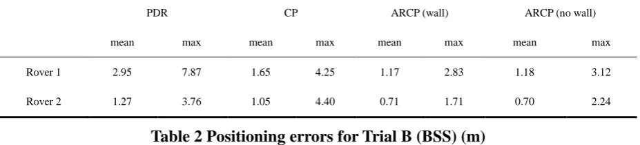
Table 1 and Table 2 list the mean and maximum positioning error throughout Trial A and 389
Trial B. Table 2 only list the error for Rover 1, as the ground truth for Rover 2 is provided by 390
the UWB system which is not accurate enough to justify the positioning accuracy of ARCP. 391
the result of non-adaptive CP with wall constraint. The CP result in Table 1 is an average of 393
integrating one of the three anchors each time and the CP result in Table 2 is an average of 394
integrating all available measurements. 395
In Trial B, as two rovers and four anchors are available, only the appropriate units are 396
selected. As anchors are not represented by particles, therefore increasing the number of 397
anchors does not affect the computation cost too much. However, the processing time is 398
reduced by at least 5% when a rover is integrated. Hence the network size is kept within four, 399
which was indicated as the effective size. 400
Table 1 Positioning errors for Trial A (NGB) (m)
PDR CP ARCP (wall) ARCP (no wall)
mean max mean max mean max mean max
Rover 1 2.95 7.87 1.65 4.25 1.17 2.83 1.18 3.12
[image:12.595.67.531.217.322.2]Rover 2 1.27 3.76 1.05 4.40 0.71 1.71 0.70 2.24
Table 2 Positioning errors for Trial B (BSS) (m)
CP ARCP (wall) ARCP (no wall)
mean max mean max mean max
Rover 1 5.30 15.99 2.03 8.61 2.28 8.98
As not enough factors are considered in CP, ARCP improves positioning accuracy by 25% in 401
Trial A and 60% in Trial B compared to CP. In Trial A, the improvement is more obvious for 402
Rover 1 as the trajectory for Rover 2 is much simpler and the wall constraint is quite 403
sufficient to constrain the inertial bias. The improvement is also much more obvious in Trial 404
B where real ranging data is implemented, which are noisier and more unstable. ARCP can 405
cope with different noise levels of real data with its threshold adjustment. 406
In both trials, the same threshold categories are applied as specified in Eq. (14). ARCP results 407
demonstrate the ability to cope with situations without map information. Wall constraint is 408
most effective in a straight long corridor without doors. However, such conditions are not 409
always met and when the state predication model is noisy, wall constraints can misplace 410
particles in the wrong room and restrict its chances of regenerating in the right location. 411
Collaborative positioning can provide sufficient constraint even in places when wall 412
constraint cannot. Therefore, the building map information can be eliminated in the ARCP 413
algorithm. This means that users can start navigating in an environment where no prior 414
information is available. 415
5 CONCLUSIONS 416
Collaborative positioning enhances positioning performance by forming a collaborative 417
network that integrates available positioning information including P2P ranging 418
measurements between nearby rovers and anchors to constrain the measurement errors. 419
Ranging measurements vary in different environments and conditions. If the wrong 420
information is integrated, position estimation may be pushed further into the wrong location 421
while reducing positioning efficiency unnecessarily. To avoid this, only the useful 422
measurements are selected and integrated into the positioning system. 423
enables the user to decide on the most effective network at each epoch. This selection is 425
based on the network geometry, network size and ranging accuracy of the units and their 426
measurements. All three elements are combined to produce a decisive factor, MDOP, which 427
helps the system to select the appropriate units as well as set the proper constraint threshold. 428
Only those units that form a good geometry while providing high ranging accuracy will be 429
used for positioning and others will be neglected. ARCP improves the positioning accuracy 430
by more than 60% for real data, while reducing the maximum error by 45%. The contribution 431
of ranging constraints also enables the system to navigate when no interior building map is 432
available. 433
By applying ARCP, the system produces results with higher accuracy and enhanced 434
robustness. It allows the system to start up without prior information on the surrounding 435
environment as long as collaborative units are found. This could be applied with Wi-Fi 436
fingerprinting to introduce more adaptivity into the positioning system enabling it to cope 437
with various difficult situations in the real world. 438
REFERENCE 439
Abdulrahim, K., Hide, C., Moore, T. and Hill, C. (2011). Aiding low cost inertial 440
navigation with building heading for pedestrian navigation. The Journal of Navigation, 441
64, 219-233. 442
Arulampalam, M.S., Maskell, S., Gordon, N. and Clapp, T. (2002). A Tutorial on Particle 443
Filters for Online Nonlinear/Non-Gaussian Bayesian Tracking. IEEE Transactions on 444
Signal Processing, 50(2), 174–188. 445
Chen, C.S., Chiu, Y.J., Lee, C.T. and Lin, J.M. (2013). Calculation of Weighted 446
Geometric Dilution of Precision. Journal of Applied Mathematics, 2013, 953048. 447
Cinefra, N. (2012) Adaptive Indoor Positioning System Based On Bluetooth Low Energy 448
RSSI. Thesis, Politecnico Di Milano, Italy. 449
Evennou F. and Marx F. (2006). Advanced Integration of WiFi and Inertial Navigation 450
Systems for Indoor Mobile Positioning. Eurasip Journal on Applied Signal Processing, 451
2006: 086706. 452
Gentile, C. and Kik, A. (2007). A Comprehensive Evaluation of Indoor Ranging using 453
Ultra-Wideband Technology. EURASIP Journal on Wireless Communications and 454
Networking, 2007, 86031. 455
Gustafsson, F., Gunnarsson, F., Bergman, N., Forssell, U., Jansson, J., Karlsson, R. and 456
Nordlund, P.J. (2002). Particle Filters for Positioning, Navigation, and Tracking. IEEE 457
Transactions on Signal Processing, 50(2), 425-437. 458
Ismail, G., Chong, C.C., Watanabe, F. and Inamura, H. (2008). NLOS identification and 459
weighted least-squares localization for UWB systems using multipath channel statistics. 460
EURASIP Journal on Advances in Signal Processing, 2008 (1), 271984. 461
Jing, H., Pinchin, J., Hill, C. and Moore, T. (2013). Wi-Fi Indoor Localisation Based on 462
Collaborative Ranging Between Mobile Users. Proceedings of the 26th International 463
Technical Meeting of the ION Satellite Division, ION GNSS+ 2013, Nashville, Tennessee. 464
Kaemarungsi, K. and Krishnamurthy, P. (2012). Analysis of WLAN’s 465
Received Signal Strength Indication for Indoor Location Fingerprinting. Pervasive and 466
Mobile Computing, 8, 292-316. 467
Analysis of UWB Technology for Indoor Positioning. Proceedings of the 2014 469
International Technical Meeting of The Institute of Navigation, ITM 2014, San Diego, 470
California. 471
Langley, R.B. (1999). Dilution of Precision. GPS world, 10(5), 52-59. 472
Lee, J.Y. and Scholtz,R.A. (2002). Ranging in a Dense Multipath Environment Using an 473
UWB Radio Link. IEEE Journal on Selected Areas in Communications, 20(9), 1677-474
1683. 475
Marano, S., Gifford, W., Wymeersch, H. and Win, M.Z. (2010). NLOS identification and 476
mitigation for localization based on UWB experimental data. IEEE Journal on Selected 477
Areas in Communications, 28 (7): 1026–1035. 478
Narzullaev, A., Yongwan, P. and Hoyoul, J. (2008). Accurate Signal Strength Prediction 479
Based Positioning for Indoor WLAN Systems. 2008 IEEE/ION Position, Location and 480
Navigation Symposium, 685-688, Monterey, CA. 481
Patwari, N., Ash, J.N., Kyperountas, S., Hero, A.O., Moses, R.L. and Correal, N.S. 482
(2005). Locating the Nodes: Cooperative Localization in Wireless Sensor Networks. 483
IEEE Signal Processing Magazine, 22(4), 54-69. 484
Penna, F., Caceres, M.A. and Wymeersch, H. (2010). Cramér-Rao Bound for Hybrid 485
GNSS-Terrestrial Cooperative Positioning, IEEE Communications Letters, 14(11), 1005– 486
1007. 487
Pinchin, J., Hide, C. and Moore, T. (2012). A Particle Filter Approach to Indoor 488
Navigation Using A Foot Mounted Inertial Navigation System and Heuristic Heading 489
Information. 2012 International Conference on Indoor Positioning and Indoor 490
Navigation (IPIN), Sydney, NSW. 491
Seo, S., Lee, B. (2010). Compact UWB Diversity Antenna for Mobile Phone 492
Applications. 2010 Asia-Pacific Microwave Conference Proceedings (APMC), pp.2268-493
2270, Yokohama, Japan. 494
Tang, S., Kubo, N. and Ohashi, M. (2012). Cooperative Relative Positioning for 495
Intelligent Transportation System. 2012 12th International Conference on ITS 496
Telecommunications, 506–511, Taipei, Taiwan. 497
von Watzdorf, S. and Michahelles, F. (2010). Accuracy of Positioning Data on 498
Smartphones. Proceedings of the 3rd International Workshop on Location and the Web, 499
Tokyo, Japan. 500
Xu, C., and Law, C.L. (2009). Experimental Evaluation of UWB Ranging Performance 501
for Correlation and ED Receivers in Indoor Environments. International Journal of 502
Hybrid Information Technology, 2(2), 37-54. 503
Weyn, M. and Schrooyen, F. (2008). A WiFi Assisted GPS Positioning Concept. 504
ECUMICT, Gent, Belgium. 505
Wymeersch, H., Lien, J. and Win, M.Z. (2009). Cooperative Localization in Wireless 506
Networks. Proceedings of the IEEE, 97(2), 427-450. 507
Wymeersch, H., Marano, S., Gifford, W.M. and Win, M.Z. (2012). A machine learning 508
approach to ranging error mitigation for UWB Localization. IEEE Transactions on 509
Communications, 60 (6): 1719–1728. 510
Yang, C. (2014). Covariance Analysis of Spatial and Temporal Effects of Collaborative 511
Symposium(PLANS), Monterey, CA. 513
Yang, C., Nguyen,T., Venable, D., White, L.M. and Siegel,R. (2009). Cooperative 514
Position Location with Signals of Opportunity. Proceedings of the IEEE 2009 National 515
Aerospace & Electronics Conference (NAECON), Dayton, OH. 516
Yao, J., Balaei, A.T., Hassan, M., Alam, N. and Dempster, A.G. (2011). Improving 517
Cooperative Positioning for Vehicular Networks. IEEE Transactions on Vehicular 518
Technology, 60(6), 2810-2823. 519
Zirari, S., Canalda, P. and Spies, F. (2009). Geometric and Signal Strength Dilution of 520