Munich Personal RePEc Archive
Maximin equilibrium
Ismail, Mehmet
Maastricht University
October 2014
Online at
https://mpra.ub.uni-muenchen.de/97322/
Mehmet Ismail
Maximin equilibrium
Maximin equilibrium
∗
Mehmet ISMAIL
†First version March, 2014. This version: October, 2014
Abstract
We introduce a new concept which extends von Neumann and Mor-genstern’s maximin strategy solution by incorporating ‘individual ra-tionality’ of the players. Maximin equilibrium, extending Nash’s value approach, is based on the evaluation of the strategic uncertainty of the whole game. We show that maximin equilibrium is invariant under strictly increasing transformations of the payoffs. Notably, every finite game possesses a maximin equilibrium in pure strategies. Considering the games in von Neumann-Morgenstern mixed extension, we demon-strate that the maximin equilibrium value is precisely the maximin (minimax) value and it coincides with the maximin strategies in two-person zerosum games. We also show that for every Nash equilibrium that is not a maximin equilibrium there exists a maximin equilibrium that Pareto dominates it. Hence, a strong Nash equilibrium is always a maximin equilibrium. In addition, a maximin equilibrium is never Pareto dominated by a Nash equilibrium. Finally, we discuss max-imin equilibrium predictions in several games including the traveler’s dilemma.
JEL-Classification: C72
Keywords: Non-cooperative games, maximin strategy, zerosum games.
∗I thank Jean-Jacques Herings for his feedback. I am particularly indebted to Ronald
Peeters for his numerous comments and suggestions about the material in this paper. I am also thankful to the audiences at Maastricht University, Paris School of Economics, CEREC Workshop at Saint-Louis University, Brussels, Paris PhD Game Theory Seminar at Institut Henri Poincar´e, Foundations of Utility and Risk Conference at Rotterdam University, The 25th International Conference on Game Theory at Stony Brook University, and International Workshop on Game Theory and Economics Applications of the Game Theory Society at the University of S˜ao Paulo, 2014. Of course, any mistake is mine.
1
Introduction
In their ground-breaking book, von Neumann and Morgenstern (1944, p. 555) describe the maximin strategy1solution for two-person games as follows:
“There exists precisely one solution. It consists of all those impu-tations where each player gets individually at least that amount which he can secure for himself, while the two get together pre-cisely the maximum amount which they can secure together. Here the ‘amount which a player can get for himself’ must be under-stood to be the amount which he can get for himself, irrespective of what his opponent does, even assuming that his opponent is guided by the desire to inflict a loss rather than to achieve a gain.”
This immediately gives rise to the following question: “What happens when a player acts according to the maximin principle but knowing that other players do not necessarily act in order to decrease his utility?”. We are going to capture this type of behavior by assuming that players are ‘individually rational’ and letting this be common knowledge among players. In other words, the contribution of the current paper can be considered as incorporating the maximin principle and ‘rationality’ of the players in one concept calling it maximin equilibrium. Our solution coincides with maximin strategy solution when the rationality assumption is dropped.
Note that it is recognized and explicitly stated by von Neumann and Morgenstern several times that their approach can be questioned by not cap-turing the cooperative side of non-zerosum games. But this did not seem to be a big problem at that time and it is stated that the applications of the theory should be seen in order to reach a conclusion.2 After more than a
half-century of research in this area, maximin strategies are indeed consid-ered to be too defensive in non-strictly competitive games in the literature. Since a maximin strategist plays any game as if it is a zerosum game, this leads to an ignorance of her opponent’s utilities and hence the preferences of her opponent. These arguments call for a revision of the maximin strategy concept in non-zerosum games.
1
We would like to note that the famous minimax (or maximin) theorem was proved by von Neumann (1928). Therefore, it is generally referred as von Neumann’s theory of games in the literature.
2
In Section 2, we present the framework and introduce the concept of max-imin equilibrium. Maxmax-imin equilibrium extends Nash’s value approach to the whole game and evaluates the strategic uncertainty of the game by follow-ing a similar method as von Neumann’s maximin strategy notion. We show that every finite game possesses a maximin equilibrium in pure strategies. Moreover, maximin equilibrium is invariant under strictly increasing trans-formations of the utility functions of the players. In Section 3, we extend the analysis to the games in von Neumann-Morgenstern mixed extension. We demonstrate that maximin equilibrium exists in mixed strategies too. We also show that for every Nash equilibrium that is not a maximin equilibrium there exists a maximin equilibrium that Pareto dominates it. Hence, a strong Nash equilibrium is always a maximin equilibrium. In addition, a maximin equilibrium is never Pareto dominated by a Nash equilibrium. Furthermore, we show by examples that maximin equilibrium is neither a coarsening nor a special case of correlated equilibrium or rationalizable strategy profiles.
In Section 4, we show that a strategy profile is a maximin equilibrium if and only if it is a pair of maximin strategies in two-person zerosum games. In particular, the maximin equilibrium value is precisely the minimax value whenever the latter exists. In Section 5, we discuss the maximin equilibrium in n-person games. All the results provided in Section 2 and in Section 3 hold in n-person games.
2
Maximin equilibrium
In this paper, we use a framework for the analysis of interactive decision making environments as described by von Neumann and Morgenstern (1944, p. 11):
does not attempt to understand those principles and the interac-tions of the conflicting interests of all participants.
For simplicity, we assume that there are two players whose finite sets of pure actions are X1 andX2 respectively. Moreover, players’ preferences over
the outcomes are assumed to be a weak order (i.e. transitive and complete) so that we can represent those preferences by the ordinal utility functionsu1, u2 :
X1×X2 →Rwhich depends on both players’ actions. As usual, the notation
x inX =X1×X2 represents a strategy profile.3 In short, a two-person
non-cooperative game Γ can be denoted by the tuple ({1,2}, X1, X2, u1, u2). We
distinguish between the game Γ and its von Neumann-Morgenstern mixed extension. Clearly, the mixed extension of a game requires more assumptions to be made and it will be treated separately in Section 3. When it is not clear from the context, we refer the original game as the pure game or the deterministic game to not to cause a confusion with the games in mixed extension. Starting from simple strategic decision making situations, we firstly introduce a deterministic theory of games in this section.4
As it is formulated and explained by von Neumann and Morgenstern (1944), playing a game is basically facing an uncertainty which can not be resolved by statistical assumptions. This is actually the crucial difference between strategic games and decision problems. Our aim is to extend von Neumann’s approach on resolving this uncertainty.
Suppose that Alfa (he) and Beta (she) make a non-binding agreement (x1, x2) inX in a two-person game. Alfa faces an uncertainty by keeping the
agreement since he does not know whether Beta will keep it. Von Neumann’s maximin method to evaluate this uncertainty is to calculate the minimum payoff of Alfa with respect to all conceivable deviations by Beta.5 That is,
Alfa’s evaluation vx1x2 (or the utility) of keeping the agreement (x1, x2) is
vx1x2 = minx′2∈X2u1(x1, x
′
2). Note that for all x2, the evaluation of Alfa for
the profile (x1, x2) is the same, i.e. vx1x2 =vx1x′2 for all x
′
2 ∈X2. Therefore,
it is possible to attach a unique evaluation vx′
1 for every strategy x
′
1 ∈ X1
of Alfa. Second step is to make a comparison between those evaluations
3
As is standard in game theory, we assume that what matters is the consequence of strategies (consequentialist approach) so that we can define the utility functions over the strategy profiles.
4
Note that all the definitions we present can be extended in a straightforward way to
n-person games which will be introduced in Section 5.
5
of the strategies. For that, von Neumann takes the maximum of all such evaluations vx′1 with respect to x′1 which yields a unique evaluation for the
whole game, i.e. the value of the game isv1 = maxx′
1∈X1vx′1. In other words,
the unique utility that Alfa can guarantee by facing the uncertainty of playing this game is v1. Accordingly, it is recommended that Alfa should choose a
strategy x∗1 ∈arg maxx′
1∈X1vx′1 which guarantees the value v1.
We would like to extend von Neumann’s method in such a way that Alfa takes into account the ‘individual rationality’ of Beta when making the evaluations and vice versa. Let us fix some terminology. As usual, a strategy
x′
i ∈ Xi is said to be a profitable deviation for player i with respect to the
profile (xi, xj) if ui(xi′, xj)> ui(xi, xj).
Definition 1. A player is called individually rational at x in X if she does
not make a non-profitable deviation from it.
We assume that players are individually rational, each player assumes that the other players are individually rational and that this is common knowledge.6 Let us construct the approach we take step by step and state
its implications. We have proposed a notion of individual rationality which allows Beta to keep her agreement or to deviate to a strategy for which she has strict incentives to do so. This is reminiscent of individual rationality constraint in economics in the sense that individually rational behavior al-ways yield higher or equal utility than individually non-rational behavior. By this assumption, Alfa can rule out non-profitable deviations of Beta from the agreement (x1, x2) which helps decreasing the level of uncertainty he is
facing. Now, Alfa’s evaluation v1(x1, x2) of the uncertainty for keeping the
agreement (x1, x2) can be defined as the minimum utility he would receive
under any individually rational behavior of Beta. Let us define the value function formally.
Definition 2. Let Γ = (X1, X2, u1, u2) be a two-person game. The function
v :X →R×R is called thevalue function of Γ if for every i6=j and for all
x= (xi, xj)∈X, the i’th component of v = (vi, vj) satisfies
vi(x) = min{ inf x′
j∈Bj(x)
ui(xi, x′j), ui(x)},
6
where the better response correspondence of player j with respect to x is defined as
Bj(x) = {x′j ∈Xj|uj(xi, x′j)> uj(x)}.
Remark. Note that for allxand all i, we haveui(x)≥vi(x). This is because
one cannot increase a payoff but can only (weakly) decrease it, by definition of the value function.
As a consequence, it is not in general true for a strategyx′
2 6=x2 that we
have the equality v1(x1, x2) = v1(x1, x′2). Because, the better response set of
Beta with respect to (x1, x2) is not necessarily the same as the better response
set of her with respect to (x1, x′2). Therefore, we cannot assign a unique value
to every strategy of Alfa anymore. Instead, the evaluation of the uncertainty can be encoded in the strategy profile as in the value notion of Nash (1950, 1951). Nash defines the value of the game (henceforth the Nash-value) to a player as the payoff that the player receives from a Nash equilibrium when all the Nash equilibria lead to the same payoff for the player. We extend Nash’s value approach to the full domain of the game, that is, we assign a value to each single strategy profile including, of course, the Nash equilibria. Notice that when a strategy profile is a Nash equilibrium, the value of a player at this profile is precisely her Nash equilibrium payoff.7 In particular,
if the Nash-value exists for a player then the player’s value of every Nash equilibria is the Nash-value of that player. As a result of assigning a value to the profiles rather than the strategies, we can no longer refer to a strategy in the same spirit of a maximin strategy since a strategy in this setting only makes sense as a part of a strategy profile as in a Nash equilibrium. But note that there are two evaluations that are attached to the profile (x1, x2), one
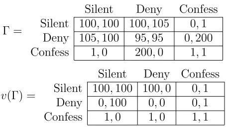
for Alfa and one for Beta since she also is doing similar inferences as him. To illustrate what a value function of a game looks like, let us consider the game Γ in Figure 1 which is played by Alfa and Beta. It can be interpreted as the prisoner’s dilemma game with an option to remain silent. Each prisoner has three options to choose from, namely remain ‘Silent’, ‘Deny’ or ‘Confess’ and let the utilities be as in Figure 1. Notice that if the strategy ‘Silent’ is removed from the game for both players then we would obtain the prisoner’s dilemma.
7
Γ =
Silent Deny Confess Silent 100,100 100,105 0,1
Deny 105,100 95,95 0,200 Confess 1,0 200,0 1,1
v(Γ) =
Silent Deny Confess Silent 100,100 100,0 0,1
[image:9.612.192.419.124.253.2]Deny 0,100 0,0 0,1 Confess 1,0 1,0 1,1
Figure 1: Prisoner’s dilemma with an option to remain silent and its value function.
Suppose that the prisoners Alfa and Beta are in the same cell and they can freely discuss what to choose before they submit their strategies. However, they will make their choices in separate cells, that is, non-binding pre-game communication is allowed. Suppose that Beta is trying to convince Alfa to make an agreement on playing, for example, the profile (Deny, Deny). Alfa would fear that Beta may not keep her agreement and may unilaterally deviate to ‘Confess’ leaving him a utility of 0. Accordingly, the value of the profile (Deny, Deny) to Alfa is 0 as shown in the bottom table in Figure 1. Now, suppose somebody offers to make an agreement on (Silent, Silent). Beta would not fear a unilateral profitable deviation ‘Deny’ of Alfa since she still gets 100 in that case. Alfa’s utility does not change too in case of a unilateral profitable deviation of Beta to ‘Deny’. In other words, the value of the profile (Silent, Silent) is (100,100) which is equal to its payoff vector in Γ.
The second and the last step is to make comparisons between the evalua-tions of the strategy profiles. We maximize the value function by the Pareto optimality principle. Now, let us formally define the maximin equilibrium.
Definition 3. Let (X1, X2, u1, u2) be a two-person game and let v = (vi, vj)
be the value function of the game. A strategy profile x = (xi, xj) where i 6= j is called maximin equilibrium if for every player i and every x′ ∈ X, vi(x′)> vi(x) implies vj(x′)< vj(x).
response correspondence of player j with respect to a profile x, i.e. Bj(x),
as being the belief of player i about player j’s possible strategies. Maximin strategy corresponds to the case in which a player’s belief about her opponent is the whole strategy set of the opponent. That is, player i does not take individual rationality of the opponent into account. With this interpretation, the maximin principle can be incorporated with stronger or weaker rationality assumptions, even with different ones for different players, by following the same method we follow in this section. Mutatis mutandis, there would not be a change in the results of this section.
Going back to the example in Figure 1, observe that the game has a unique Nash equilibrium (Confess, Confess) with a payoff vector of (1,1). Observe also that the profile (Silent, Silent) is the Pareto dominant profile of the value function, so it is the maximin equilibrium with a value of (100,100). More-over, the maximin equilibrium (Silent, Silent) has another property which may deserve attention. Suppose that players agree on playing it. Alfa has a chance to make a unilateral profitable deviation to ‘Deny’ but he cannot rule out a potential profitable deviation of Beta to the strategy ‘Deny’. If this happens, Alfa would receive 95 which is strictly less than what he would receive if he did not deviate to ‘Deny’. But Beta is also in the exactly same situation. As a result, it seems that none of them would actually deviate from the agreement (Silent, Silent).
We obtain maximin equilibrium by evaluating each single strategy profile in a game. One of the reasons of extending Nash (1950)’s value argument is the following. A Nash equilibrium is solely based on the evaluation of the outcomes that might occur as a consequence of a player choosing one strategy with the outcomes that might occur as a consequence of an opponent choos-ing another strategy. Therefore, it seems to be quite questionable whether the Nash-value represents an evaluation of the strategic uncertainty of the
whole game or only of these outcomes. Since a Nash equilibrium completely
100 99 · · · 3 2 100 100,100 97,101 · · · 1,5 0,4
[image:11.612.211.410.126.222.2]99 101,97 99,99 · · · 1,5 0,4 ... ... ... . .. ... ... 3 5,1 5,1 · · · 3,3 0,4 2 4,0 4,0 · · · 4,0 2,2
Figure 2: Traveler’s dilemma
In the traveler’s dilemma, the payoff function of a playeriif she plays xi
and her opponent plays xj is defined as ui(xi, xj) = min{xi, xj}+r·sgn(xj− xi) for all xi, xj inX ={2,3, ...,100} wherer >1 determines the magnitude
of reward and punishment which is 2 in the original game. Regardless of the magnitude of the reward/punishment, the unique Nash equilibrium is (2,2) which is also the unique outcome of the process of iterated elimination of strictly dominated strategies.
It is shown by many experiments that players do not on average choose the Nash equilibrium strategy and that changing the reward/punishment parameter r affects the behavior observed in experiments. Goeree and Holt (2001) found that when the reward is high, 80% of the subjects choose the Nash equilibrium strategy but when the reward is small about the same percent of the subjects choose the highest. This finding is a confirmation of Capra et al. (1999). There, play converged towards the Nash equilibrium over time when the reward was high but converged towards the other extreme when the reward was small. On the other hand, Rubinstein (2007) found (in a web-based experiment without payments) that 55% of 2985 subjects choose the highest amount and only 13% choose the Nash equilibrium where the reward was small. These results are actually not unexpected. The irony is that if both players choose almost8 any ‘irrational’ strategy but their Nash
equilibrium strategy, then they both get strictly more payoff than they would get by playing the Nash equilibrium. Moreover, the strategy ‘2’ is the worst reply in all those cases. In fact, the Nash equilibrium is the only profile which has this property in the game.
To find the maximin equilibria we first need to compute the value of the traveler’s dilemma. The value function of player i is given by
8
If one modifies the payoffs of the game such that ui(xi,3) = 2.1 and ui(xi,4) = 2.1
vi(xi, xj) =
xj −2, if xi > xj for xi ∈X xi−3, if xi =xj for xi ∈X\ {2}
2, if xi =xj = 2
xi−5, if xi < xj for xi ∈X\ {4,3,2}
0, if xi < xj for xi ∈ {4,3,2}.
Observe that the maximum of the value function is (97,97) which is assumed at (100,100). Hence, the profile (100,100) is the unique maximin equilibrium and (97,97) is the value of it. Note that as the reward parameter
rincreases, the value of the maximin equilibrium decreases. Whenris higher than or equal to 50, the unique maximin equilibrium becomes the profile (2,2) which is also the unique Nash equilibrium of the game. This seems to explain both the convergence of play to (100,100) when the reward is small, and the convergence of play to (2,2) when the reward is big.
An ordinal utility function is unique up to strictly increasing transforma-tions. Therefore, it is crucial for a solution concept (which is defined with respect to ordinal utilities) to be invariant under those operations. The fol-lowing proposition shows that maximin equilibrium possesses this property.
Proposition 1. Maximin equilibrium is invariant under strictly increasing
transformations of the utility function of the players.
Proof. Let Γ = (Xi, Xj, ui, uj) and ˆΓ = (Xi, Xj,uˆi,uˆj) be two games such
that ˆui and ˆuj are strictly increasing transformations of ui and uj
respec-tively. Firstly, we show that the components ˆvi and ˆvj of the value function
ˆ
v are strictly increasing transformations of the components vi and vj of v,
respectively. Notice that Bj(x) = ˆBj(x), that is
{x′j ∈Xj|uj(xi, x′j)> uj(x)}={x′j ∈Xj|uˆj(xi, x′j)>uˆj(x)}.
It implies that arg minx′
j∈Bj(x)ui(xi, x
′
j) = arg minx′
j∈Bˆj(x)uˆi(xi, x
′
j) such that vi(x) = min{ui(xi,x¯j), ui(x)} and ˆvi(x) = min{uˆi(xi,x¯j),uˆi(x)} for some
¯
xj ∈arg minx′j∈Bj(x)ui(xi, x′j). Since ˆui is a strictly increasing transformation
of ui, we have either vi(x) = ui(xi,x¯j) if and only if ˆvi(x) = ˆui(xi,x¯j) or vi(x) = ui(x) if and only if ˆvi(x) = ˆui(x) for all xi, xj and all ¯xj. It follows
that showing vi(x) ≥ vi(x′) if and only if ˆvi(x) ≥ vˆi(x′) is equivalent to
showing ui(x)≥ui(x′) if and only if ˆui(x)≥uˆi(x′) for allx, x′ inX which is
a b c a 1,1 3,3 1,1 b 3,1 3,3 3,4 c 3,3 1,3 4,1
a b c I
[image:13.612.173.449.129.200.2]a 1,1 3,3 1,1 −1,0 b 3,1 3,3 3,4 −1,0 c 3,3 1,3 4,1 −1,0 I 0,−1 0,−1 0,−1 0,0
Figure 3: Two games Γ (left) and Γ′ (right). In the former, the payoffs to the
Nash equilibria and to the maximin strategies are the same while it changes in the latter.
Secondly, a profile y is a Pareto optimal profile with respect to v if and only if it is Pareto optimal with respect to ˆv because each vi is a strictly
increasing transformation of ˆvi. As a result, the set of maximin equilibria of
Γ and ˆΓ are the same.
The following proposition shows the existence of maximin equilibrium in pure strategies. This may be especially a desired property in games where players cannot or are not able to use a randomization device. It might be also the case that a commitment of a player to a randomization device is implausible. In those games, we can make sure that there exists at least one maximin equilibrium.
Theorem 1. Every finite game has a maximin equilibrium in pure strategies.
Proof. Since Pareto dominance relation is reflexive and transitive a Pareto optimal strategy profile with respect to the value function of a finite game always exists.
Moreover, maximin equilibria are invariant under addition of “irrelevant strategies” to a game. In other words, suppose that we add new strategies to a game Γ calling the new game Γ′ and that all new outcomes are strictly
less preferred to the outcomes in Γ. Then the set of maximin equilibria in Γ′ are the same as the ones in Γ. For example, let us consider the games
Although the point we want to make is different, it is of importance to note the historical discussion about this type of games where the Nash equilibria payoffs are equal to the payoffs that can be guaranteed by play-ing maximin strategies. Harsanyi (1966) postulates that players should use their maximin strategies in those games which he calls unprofitable. Luce and Raiffa (1957) and Aumann and Maschler (1972) argue that maximin strategies seem preferable in those games. In short, in the games similar to Figure 3, the arguments supporting maximin strategies are so strong that it led some game theory giants to prefer them over the Nash equilibria of the game. These arguments, however, may disappear when we add an ‘irrelevant’ strategy ‘I’ to the game for both players. Notice that the Nash equilibria in Γ are also Nash equilibria in Γ′. By contrast, the maximin strategies in Γ
disappears. That is, the new maximin strategy in Γ′ is ‘I’ for both players
and it guarantees zero.9 On the other hand, all maximin equilibria including
(b,b) remains unchanged in Γ′.
3
The mixed extension of games
3.1
Maximin equilibrium
The mixed extension of a two-player non-cooperative game is denoted by (∆X1,∆X2, u1, u2) where ∆Xiis the set of all simple probability distributions
over the set Xi.10 It is assumed that the preferences of the players over
the strategy profiles satisfy weak order, continuity and the independence axioms.11 As a result, those preferences can be represented by von
Neumann-Morgenstern (expected) utility functions u1, u2 : ∆X1×∆X2 →R. A mixed
strategy profile is denoted by p∈∆X where ∆X = ∆X1×∆X2.
We do not need another definition for maximin equilibrium with respect to mixed strategies; one can just interpret the strategies in Definition 2 and in Definition 3 as being mixed. Harsanyi and Selten (1988, p. 70) argue that invariance with respect to positive linear transformations of the utilities is a fundamental requirement for a solution concept. The following proposition
9
It is clear that whichever game we consider, it is possible to make maximin strategies disappear by this way.
10
For a detailed discussion of the mixed strategy concept, see Luce and Raiffa (1957, p. 74)’s influential book in game theory.
11
shows that maximin equilibrium has this property.
Proposition 2. The maximin equilibria of a game in mixed extension is
unique up to positive linear transformations of the utilities.
We omit the proof since it follows essentially the same steps as the proof of Proposition 1. The following lemma illustrates a useful property of the value function of a player.
Lemma 1. The value function of a player is upper semi-continuous.
Proof. In several steps, we show that the value function vi of player i in a
game Γ = (∆X1,∆X2, u1, u2) is upper semi-continuous.
Firstly, we show that the better reply correspondenceBj : ∆Xi×∆Xj ։
∆Xj is lower hemi-continuous. For this, it is enough to show the graph of Bj defined as follows is open.
Gr(Bj) ={(q, pj)∈∆X×∆Xj|pj ∈Bj(q)}.
Gr(Bj) is open in ∆X ×∆Xj if and only if its complement is closed. Let
[(pj, qi, qj)k]∞k=1be a sequence in [Gr(Bj)]c = (∆X×∆Xj)\Gr(Bj) converging
to (pj, qi, qj) wherepkj ∈/ Bj(qk) for allk. That is, we haveuj(pkj, qik)≤uj(qk)
for all k. Continuity of uj implies that uj(pj, qi) ≤ uj(q) which means pj ∈/ Bj(q). Hence [Gr(Bj)]c is closed which implies Bj is lower hemi-continuous.
Next, we define ˆui : ∆Xi ×∆Xj ×∆Xj → R by ˆui(qi, qj, pj) =ui(pj, qi)
for all (qi, qj, pj) ∈ ∆Xi ×∆Xj ×∆Xj. Since ui is continuous, ˆui is also
continuous. In addition, we define ¯ui : Gr(Bj) → R as the restriction of ˆui
to Gr(Bj), i.e. ¯ui = ˆui|Gr(Bj). The continuity of ˆui implies the continuity of
its restriction ¯ui which in turn implies ¯ui is upper semi-continuous.
By the theorem of Berge (1959, p. 115)12 lower hemi-continuity of B
j
and lower semi-continuity of −u¯i : Gr(Bj) → R implies that the function
−v¯i : ∆Xi ×∆Xj → R defined by −v¯i(q) = suppj∈Bj(q)−u¯i(pj, q) is lower
semi-continuous.13 It implies that the function ¯v
i(q) = infpj∈Bj(q)u¯i(pj, q) is
upper semi-continuous.
As a result, the value function of playeridefined byvi(q) = min{v¯i(q), ui(q)}
is upper semi-continuous because the minimum of two upper semi-continuous functions is also upper semi-continuous.
12
We follow the terminology, especially the definition of upper hemi-continuity, presented in Aliprantis and Border (1994, p. 569).
13
A B C D A 2,2 0,0 1,1 0,0 B 0,0 90,80 3,3 90,90 C 1,100 100,80 −1,−1 −3,−2 D 3,1 75,0 0,0 230,0
Figure 4: A game Γ in mixed extension.
The following theorem shows that maximin equilibrium exists also in mixed strategies.
Theorem 2. Every finite game in mixed extension has a maximin
equilib-rium.
Proof. Let us definevmax
i = arg maxq∈∆X vi(q) which is a non-empty compact
set because ∆X is compact and vi is upper semi-continuous by Lemma 1.
Since vmax
i is compact and vj is also upper semi-continuous the set vmaxij =
arg maxq∈vmax
i vj(q) is non-empty and compact. Clearly, the profiles in v
max ij
are Pareto optimal with respect to the value function which means vmax ij is
a non-empty compact subset of the set of maximin equilibria in the game. Similarly, one may show that the setvmax
ji is also a non-empty compact subset
of the set of the maximin equilibria.
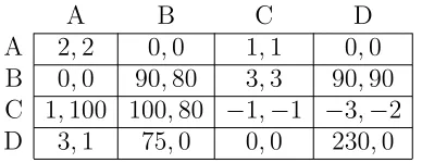
For an illustrative example, let us consider the game in Figure 4 played by Alfa and Beta. Observe that it has a unique Nash equilibrium (D,A) whose payoff vector is (3,1). An interesting phenomenon occurs if we change, ceteris paribus, the payoff ofu1(C, D) from−3 to−4. Let us call the new game Γ′. It
has the same pure Nash equilibrium (D,A) as Γ plus two mixed ones. Among them, the Pareto dominant Nash equilibrium is [(0,4146,465,0),(0,4752,0,525)] whose expected payoff vector is (90,80).14 Note that by passing from Γ′ to
Γ we just slightly increase Alfa’s relative preference of the worst outcome (C,D) with respect to the other outcomes and also that ordinal preferences remain the same. From economics viewpoint the question arises: Should ceteris paribus effect of increasing the payoff of u1(C, D) from −4 to −3 be
substantially high with respect to the solutions of the two games? According to maximin equilibrium the answer is negative. For instance, there is a
14
F O F 2,1 0,0 O 0,0 1,2
F O
[image:17.612.226.391.125.174.2]F 2,2 0,1 O 0,1 1,3
Figure 5: Two strategically equivalent battle of the sexes games.
maximin equilibrium [B,(0,2831,0,313)] in Γ whose value is approximately 80.9 for both players. Moreover, it remains to be a maximin equilibrium with the same value in Γ′.15 Actually, it turns out that the value of a player at a
strategy profile is continuous as a function of her utility at this profile. The following proposition shows this result formally.
Proposition 3. Let Γ = (∆X1,∆X2, u1, u2) be a game and fix a strategy
profilep∈∆X1×∆X2. Everything else being equal, if we increase (decrease)
ui(p) by ǫ >0 then vi(p) weakly increases (decreases) by at most ǫ.
Proof. There are two cases. Case 1: Define infp2∈B2(p)u1(p1, p2′) = u1 and
suppose that u1(p) > u1 so that v1(p) = u1. Then, for the new value v1′
we still have v′
1(p) = u1 so v1(p) remains unchanged. Case 2: Suppose that
u1(p)≤u1 so thatu1(p) =v1(p). Ifu1 < u1(p) +ǫthen we havev1′(p) =u1 <
u1(p) +ǫ=v1(p) +ǫ. Ifu1 ≥u1(p) +ǫthenv1′(p) =u1(p) +ǫ=v1(p) +ǫ. The
case when the value of a player decreases can be shown by following similar steps as above.
Since the above proposition is true for every profile, it also holds for maximin equilibria. Note also that increasing the utility of a player at a profile does not affect the value of the player at the other profiles. Hence, suppose we increase Alfa’s payoff of any profile byǫ >0 in a game Γ and call the new game Γ′. Then it is not possible to find a maximin equilibrium pin
Γ so that Alfa’s value at pis strictly larger than Alfa’s value of any maximin equilibrium in Γ′.
For another illustrative example consider the battle of the sexes game presented on the left in Figure 5. Alfa and Beta have each two choices to make between ‘Opera’ (O) and ‘Football’ (F). There are two maximin equilibria in
15
this game which are (O,O) and (F,F) that are also Nash equilibria. Given the information, it does not seem possible to define a unique ‘solution’ to this game. One might be tempted to propose that the solution of this game should be the mixed Nash equilibrium [(2
3, 1 3),(
1 3,
2
3)] whose expected payoff vector
is (23,23) because it seems more ‘distinguishable’. This temptation, however, may disappear when we consider the game on the right in Figure 5. In this game, it seems that the profile (F,F) is also ‘distinguishable’ and it Pareto dominates the mixed Nash equilibrium [(23,13),(31,23)] whose payoff is (23,53). Notice that the payoffs of Beta in the second game is just a positive linear transformation of the payoffs in the first game. Therefore, these two games must have the same solution in whatever way we define it; assuming that a solution must be invariant with respect to different numerical representation of the utilities.
3.2
The relation of maximin equilibrium with the other
concepts
Nash equilibrium is probably the most well-known solution concept in game theory. Let us state Nash (1950)’s path-breaking theorem formally: Every finite game in mixed extension possesses at least one strategy profile psuch that pi ∈ arg maxp′i∈∆Xiui(p
′
i, pj). The following two propositions illustrate
Pareto dominance relation between Nash equilibrium and maximin equilib-rium.
Proposition 4. For every Nash equilibrium that is not a maximin
equilib-rium there exists a maximin equilibequilib-rium that Pareto dominates it.
Proof. If a Nash equilibriumq in a game is not a maximin equilibrium, then there exists a maximin equilibriumpwhose valuev(p) Pareto dominatesv(q). It implies that p Pareto dominates q in the game since the payoff vector of the Nash equilibrium q is the same as its value.
The following corollary shows that a strong Nash equilibrium (Aumann, 1959) is always a maximin equilibrium.
Corollary 1. A strong Nash equilibrium is a maximin equilibrium.
Proposition 5. A maximin equilibrium is never Pareto dominated by a Nash equilibrium.
Proof. By contradiction, suppose that a Nash equilibriumqPareto dominates
a maximin equilibriump. It implies that the value ofqalso Pareto dominates the value of p. But this is a contradiction to our supposition that p is a maximin equilibrium.
The two propositions above are closely linked but one does not follow from the other. Proposition 4 does not exclude the existence of a Nash equilibrium that is both Pareto dominated by a maximin equilibrium and Pareto dominates another maximin equilibrium. Proposition 5 shows that this is not the case.
Note that maximin equilibrium is distinct from rationalizable strategy profiles (Bernheim, 1984 and Pearce, 1984) and correlated equilibrium (Au-mann, 1974) since maximin equilibrium is not necessarily an outcome of the iterated elimination of strictly dominated strategies. As discussed earlier, the profile (2,2) is the only outcome of this process in the traveler’s dilemma, but it is not a maximin equilibrium.
One might wonder whether there is a relationship between the maximin (minimax) decision rule16 in decision theory and the maximin equilibrium.
Imagine a one-player game in which the decision maker is to make a choice between several gambles. In that case, maximin equilibrium boils down to expected utility maximization just like maximin strategies and Nash equi-librium. In other words, the decision maker has to choose the gamble with the highest expected utility. However, according to maximin decision rule, a decision maker has to choose the gamble which maximizes the utility with respect to the worst state of the world (whose outcome is the minimum) even though the probability assigned to it is very small.
4
Zerosum games
Two-person zerosum games are both a historically and theoretically impor-tant class in game theory. We illustrate the relationship between the equilib-rium solution of von Neumann (1928) and the maximin equilibequilib-rium in this class of games. The following lemma will be useful for the next proposition.
16
Lemma 2. Let(Y1, Y2, u1, u2) be a two-person zerosum game whereYi is not
necessarily finite. Then vi(yi, yj) = infyj′∈Yjui(yi, y
′
j) for each i6=j.
Proof. Suppose that there exists ¯yj ∈Yj such that ¯yj ∈arg miny′
j∈Yjui(yi, y
′ j).
Then vi(yi, yj) = minyj′∈Yjui(yi, y
′
j) =ui(yi,y¯j). Suppose, otherwise, that for
all y′
j ∈ Yj there exists yj′′ ∈ Yj such that ui(yi, yj′′) < ui(yi, y′j). It implies
that vi(yi, yj) = infyj′:ui(yi,y′j)<ui(yi,yj)ui(yi, y
′
j) = infyj′∈Yjui(yi, y
′ j).
The following proposition shows that a strategy profile is a maximin equi-librium if and only if it is a pair of maximin strategies in zerosum games.
Proposition 6. Let(Y1, Y2, u1, u2)be a two-person zerosum game whereYi is
not necessarily finite. A profile (y∗
1, y2∗)∈Y1×Y2 is a maximin equilibrium if
and only if y∗
1 ∈arg maxy1infy2u1(y1, y2) and y
∗
2 ∈arg maxy2infy1u2(y1, y2).
Proof. ‘⇒’ Firstly, we show that the value of a maximin equilibrium (y∗
1, y∗2)
must be Pareto dominant in a zerosum game. By contraposition, suppose that its value is not Pareto dominant, i.e. there is another maximin equi-librium (ˆy1,yˆ2) such that vi(y1∗, y2∗)> vi(ˆy1,yˆ2) and vj(y1∗, y2∗)< vj(ˆy1,yˆ2) for
i6=j. By Lemma 2, we havev1(y1∗, y2∗) =v1(y1∗,yˆ2) andv2(ˆy1,yˆ2) =v2(y1∗,yˆ2).
It implies that the value of (y∗
i,yˆj) Pareto dominates the value of (y1∗, y∗2)
which is a contradiction to our supposition that (y∗
1, y2∗) is a maximin
equi-librium. Since the value of (y∗
1, y2∗) is Pareto dominant, each strategy is a
maximin strategy of the respective players. ‘⇐’ Suppose that for eachiwe havey∗
i ∈arg maxyiinfyjui(yi, yj). By Lemma
2, it implies that for all (y′
1, y2′)∈Y1×Y2 and for eachi we havevi(y1∗, y∗2)≥ vi(y1′, y2′) . Hence the value of (y1∗, y2∗) is Pareto dominant which implies that
it is a maximin equilibrium.
Corollary 2. In a zerosum game, maximin equilibrium and equilibrium
co-incide whenever an equilibrium exists.
As a result, maximin equilibrium indeed generalizes the maximin strategy concept of von Neumann (1928) from zerosum games to non-zerosum games. To sum up, existence of an equilibrium in a zerosum game implies that equi-libria and maximin equiequi-libria coincide. But note that maximin equilibrium may exists even though an equilibrium does not exists. In any case, maximin equilibrium is a pair of maximin strategies in zerosum games.
Beta
Beta
l
Beta
r
1 0 0 −1
· · · ·Alfa· · · ·
1 −1 0 10
[image:21.612.201.414.125.241.2]
Figure 6: The game (∆X,∆Xl∪∆Xr, u,−u).
between the left door and the right door. She is not allowed to commit to a randomization device nor is she allowed to use a device by herself for this choice. If she picks the left door, they will play the game at the left of Figure 6. If she picks the right door, they will play the game at the right of Figure 6. At this stage, players may commit to mixed strategies by submitting them on a computer. Alfa will not be informed which normal-form game he is playing. This situation can be represented by the zerosum game (∆X,∆Xl∪∆Xr, u,−u) in which Alfa chooses a mixed strategy in ∆X
and Beta chooses a mixed strategy in either ∆Xl or in ∆Xr.
Notice that there is no equilibrium in this game. There are, however, maximin strategies for each player that are (1112,121) ∈ ∆X guaranteeing −121 and (0,1) ∈ ∆Xl guaranteeing 0. By Proposition 6, this pair is also the
unique maximin equilibrium whose payoff vector is (−1 12,
1
12). However,
max-imin equilibrium does not necessarily say that this is the payoff that players should expect by playing their part of the maximin equilibrium. Rather, the unique maximin equilibrium value of this game is (−1
12,0). In other words,
the unique value of the game to Alfa is −121 given the individual rationality of Beta and the unique value of the game to Beta is 0 given the individual rationality of Alfa. If the television programmer modifies the game so that Beta is allowed to commit to a randomization device in the beginning, then the game would have an equilibrium [(1112,121),(0,1112,0,121)] which is also a maximin equilibrium. Note that Beta is now able to guarantee the payoff 1
12.
Be-L R L 0,0 2,−2 R 3,−3 1,−1
Figure 7: A zerosum game.
fore the coin toss, the maximin strategy (1 2,
1
2) of Alfa guarantees the highest
expected payoff of 1.5 in the mixed extension. However, after the coin toss Alfa still needs to make a decision whether playing according to the outcome of the toss or not. Actually, for both players playing strategy R guarantees more than playing L after the randomization. Hence the maximin equilib-rium of this deterministic game is (R,R) whose value is (1,−2) whereas the values of the profiles (L,L),(L,R) and (R,L) are (0,−3),(0,−2) and (1,−3) respectively. Note that if players are allowed to use mixed strategies then the maximin equilibrium is [(12,12),(14,34)].
5
Maximin equilibrium in
n
-person games
Firstly, we define the value function. For this, we replace the wayviis written
in Definition 2 to vi(p) = min{infp−′i∈B−i(p)ui(pi, p′−i), ui(p)} whereB−i(p) is
defined as follows. Firstly for each S ⊆N \ {i}and each p∈∆X define
BS
−i(p) = {(ˆpS, p−S)∈∆X−i|uk(ˆpk, p−k)> uk(p) for all k ∈S}. BS
−i(p) is the set of (n −1)-tuple strategy profiles in which the players in S make a unilateral profitable deviation with respect to p. To represent all such profiles for all S ⊆ N \ {i}, we define the correspondence B−i(p) =
S
S⊆N\{i}B−Si(p). Accordingly, a strategy profile is a maximin equilibrium if
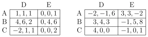
its value is not Pareto dominated. Moreover, every result in Section 2 and in Section 3 is valid in n-person games. The proofs are essentially the same as the ones given in Section 2 and in Section 3.
D E A 1,1,1 0,0,1 B 4,6,2 0,4,6 C −2,1,1 0,0,2
D E
[image:23.612.182.434.137.200.2]A −2,−1,6 3,3,−2 B 3,4,3 −1,5,8 C 4,0,0 −1,0,1
Figure 8: A three player game where player 3 chooses between the matrices L (left) and R (right).
(0.71,2.12,2.39). Note that the Nash-value of Juliet is the highest so she seems to be the most advantageous player in the game. Suppose that Juliet naively thinks that she is doing the ‘best’ by playing her part of the Nash equi-librium. Even without any communication, Alfa and Beta may unilaterally deviate from the Nash equilibrium to the strategies ‘B’ and ‘C’ respectively after which they both receive (3.68 and 5.36, respectively) strictly more than their Nash equilibrium payoff which causes the Nash equilibrium to “break down”. As a result, Juliet ends up with a strictly less payoff (2.32) than her payoff at the Nash equilibrium.
Notice that potential deviations of Alfa and Beta are costless, because the strategy ‘B’ of Alfa is a best response to the Nash equilibrium strategies of the other players and ‘D’ of Beta is also best response to the Nash equilibrium strategies of the others. Note also that these deviations are not coalitional deviations. We do not claim that when a player deviates, the other also must deviate. It could very well be the case that Alfa unilaterally deviates to ‘B’ but Beta sticks to her Nash equilibrium strategy or vice versa. In this case, Alfa would not lose anything. What ‘breaks the Nash equilibrium down’ is the very possibility that by anticipating the situation Beta also deviates to ‘D’. In addition, holding the Nash equilibrium strategy (0.68,0.32) of Juliet fixed, the profile (B,D) is the Pareto dominant Nash equilibrium in the game played by Alfa and Beta! Consequently, the very argument that players have no incentive to unilaterally deviate at a Nash equilibrium does not hold in this example. Since every pure strategy in the support of a mixed Nash equilibrium is a best response, every mixed Nash equilibrium and even sometimes a pure Nash equilibrium may, potentially, have the problem described above in n-person games.17
17
(Bern-In fact, von Neumann and Morgenstern (1944, p. 32) strikingly anticipate the problem we discussed above years before the emergence of Nash equilib-rium: “Imagine that we have discovered a set of rules for all participants to be termed as “optimal” or “rational” each of which is indeed optimal provided that the other participants conform. Then the question remains as to what will happen if some of the participants do not conform. If that should turn out to be advantageous for them and, quite particularly, disadvantageous to the conformists then the above “solution” would seem very questionable. We are in no position to give a positive discussion of these things as yet but we want to make it clear that under such conditions the “solution,” or at least its motivation, must be considered as imperfect and incomplete.”
Maximin equilibrium can be modified to incorporate coalitions in n -person games, we just need to define the better reply correspondence allowing coalitional profitable deviations and define the value function with respect to this. Accordingly, a profile is called strong maximin equilibrium if its value is not Pareto dominated. By the same argument in Theorem 1, it exists in pure strategies in the deterministic game. Regarding the mixed exten-sion of games, one may show the existence of strong maximin equilibrium by following the similar steps as in Lemma 1 and in Theorem 2. Regarding the three-player game above, both the maximin equilibrium and the strong maximin equilibrium is the profile (B,D,(12,12)) whose value is (3,4,2.5). In other words, by playing their part of the maximin equilibrium each player guarantees her value under any profitable deviation of the other players.
6
Conclusion
In this paper, we extended von Neumann’s maximin strategy solution in strategic games by incorporating individual rationality of the players. Max-imin equilibrium extends Nash’s value approach to the whole game and eval-uates the strategic uncertainty of the game by following a similar method as von Neumann’s maximin strategy notion. We showed that maximin equi-librium is invariant under strictly increasing transformations of the payoffs. Notably, every finite game possesses a maximin equilibrium in pure strate-gies.
Considering the games in von Neumann-Morgenstern mixed extension, we demonstrated that maximin equilibrium exists in mixed strategies as well. Moreover, we showed that a strategy profile is a maximin equilibrium if and only if it is a pair of maximin strategies in two-person zerosum games. In particular, a maximin equilibrium and an equilibrium coincide whenever the latter exist in those games. Furthermore, we showed that for every Nash equilibrium that is not a maximin equilibrium there exists a maximin equilibrium that Pareto dominates it. Hence, a strong Nash equilibrium is always a maximin equilibrium. Besides, a maximin equilibrium is never Pareto dominated by a Nash equilibrium. The concept introduced in this paper opens up several research directions such as further exploration in extensive form games and in repeated games.
References
Aliprantis, C. and K. Border (1994).Infinite Dimensional Analysis: A Hitch-hiker’s Guide.
Aumann, R. J. (1959). Acceptable points in general cooperative n-person games. In R. D. Luce and A. W. Tucker (Eds.),Contribution to the theory
of game IV, Annals of Mathematical Study 40, pp. 287–324. University
Press.
Aumann, R. J. (1974). Subjectivity and correlation in randomized strategies.
Journal of Mathematical Economics 1(1), 67–96.
Aumann, R. J. (1976). Agreeing to disagree. The Annals of Statistics 4(6), pp. 1236–1239.
Aumann, R. J. and M. Maschler (1972). Some thoughts on the minimax principle. Management Science 18(5-Part-2), 54–63.
Basu, K. (1994). The traveler’s dilemma: Paradoxes of rationality in game theory. The American Economic Review 84(2), 391–395.
Berge, C. (1959). Espaces topologiques: Fonctions multivoques. Dunod.
Bernheim, B. D., B. Peleg, and M. D. Whinston (1987). Coalition-proof Nash equilibria i. concepts. Journal of Economic Theory 42(1), 1–12.
Capra, C. M., J. K. Goeree, R. Gomez, and C. A. Holt (1999). Anomalous behavior in a traveler’s dilemma? American Economic Review 89(3), 678–690.
Fishburn, P. (1970). Utility theory for decision making. Publications in operations research. Wiley.
Gilboa, I. and D. Schmeidler (1989). Maxmin expected utility with non-unique prior. Journal of Mathematical Economics 18(2), 141–153.
Goeree, J. K. and C. A. Holt (2001). Ten little treasures of game theory and ten intuitive contradictions. American Economic Review 91(5), 1402– 1422.
Harsanyi, J. C. (1966). A general theory of rational behavior in game situa-tions. Econometrica 34(3), pp. 613–634.
Harsanyi, J. C. and R. Selten (1988). A General Theory of Equilibrium
Selection in Games. MIT Press.
Lewis, D. (1969). Convention: a philosophical study. Harvard University Press.
Luce, R. and H. Raiffa (1957). Games and Decisions: Introduction and
Crit-ical Survey. Dover books on advanced mathematics. Dover Publications.
Nash, J. F. (1950). Non-cooperative games. PhD Diss. Princeton University.
Nash, J. F. (1951). Non-cooperative games. Annals of Mathematics 54(2), 286–295.
Pearce, D. G. (1984). Rationalizable strategic behavior and the problem of perfection. Econometrica 52(4), pp. 1029–1050.
Rubinstein, A. (2007). Instinctive and cognitive reasoning: A study of re-sponse times. The Economic Journal 117(523), 1243–1259.
von Neumann, J. (1928). Zur Theorie der Gesellschaftsspiele. Mathematische
von Neumann, J. and O. Morgenstern (1944). Theory of Games and
Eco-nomic Behavior (1953, Third ed.). Princeton University Press.