Sequential Variable Selection as Bayesian Pragmatism in Linear Factor Models

(1)

Sequential Variable Selection as Bayesian Pragmatism in

Linear Factor Models

John Knight1_{, Stephen Satchell}2_{, Jessica Qi Zhang}3

1_{Department of Economics, University of Western Ontario, Ontario, Canada} 2_{Department of Finance, University of Sydney, Sydney, Australia} 3_{Department of Accounting and Finance, University of Greenwich, London, UK}

Email: [email protected], [email protected], [email protected]

Received January 10, 2013; revised February 9, 2013; accepted February 20, 2013

ABSTRACT

We examine a popular practitioner methodology used in the construction of linear factor models whereby particular factors are increased or decreased in relative importance within the model. This allows model builders to customise models and, as such, reflect those factors that the client and modeller may think important. We call this process Prag- matic Bayesianism (or prag-Bayes for short) and we provide analysis which shows when such a procedure is likely to be successful.

Keywords: Linear Factor Models; Bayesian Statistics; Sequential Regression

1. Introduction

The purpose of this paper is to investigate statistical procedures frequently used by practitioners to build factor models. In particular, we are interested in the variable selection methodologies that are used to give a particular returns model a particular style and nature. For example, in the context of global models, one may wish the model to depend more or less upon domestic factors such as country’s indices rather than, say, global factors such as currency or world equity and bond markets. Likewise at the domestic level, one may want one’s model to be built around styles (value, growth etc.) rather than industries or sectors—alternatively, the opposite may be preferred. The literature on this topic is very sparse. We present a brief survey of alternative approaches. The problem can be viewed as a practical alternative to well-known Baye- sian procedures, such as Jorion’s (1986) [1] Bayes Stein adjustment and Black-Litterman’s BL model (1991, 1992) [2,3]. These models are both examples of Bayesian adjustment which effectively updates currently held opinions with data to form new opinions. Satchell and Scow- croft (2000) [4] also present details of Bayesian portfolio construction procedures based on Black-Litterman models. The essential idea in this process is to have a prior distribution over expected returns or over the regression Betas. In either case, one needs to specify hyperparame- ters which are, in practice, very troublesome. The procedure we advocate, and which is used by practitioners, is to convert beliefs about the magnitude of betas into procedures of sequential regression.

In Section 2 we shall describe how this is done in practice and how it could be analysed in theory. In Section 3 we shall present conditions under which these methodologies should work. Section 4 presents some empirical results. Conclusions and further discussion are presented in Section 5.

2. Theorem

There are a number of procedures that can be used to facilitate one factor being preferred to another. Here we shall assume that our return series is denoted by the n × 1 vector y, and the two factors over which we may have preferences are denoted by X₁ and X₂ respectively, both n × 1 vectors.

Letting _nX_₂



X X1, 2



, we will facilitate calculations later by making the following assumption:

1 1

X X 



 

   

 

Our “true” model is

1 1 2 2

yX X  u (1) where y and u are n× 1 vectors, β1 and β2 are scalars and



2



~ 0, N

u N  I .

This is obviously a simplification of the general case, but little is lost in so doing and it allows us to focus on the essential features of the problem. We now define the sequential variable selection method (SVSM), which is the essential component of the prag-Bayes approach.

(2)

procedure. If you want variable 1 to “explain” more of y

asset returns than variable 2, you regress variable 1 first in a univariate regression. The coefficient for variable 2 is then calculated by regressing the residual of y on variable 1 upon the residual of variable 2 on variable 1.

The question we wish to ask is: under what circumstances will this procedure lead to a larger estimated ex- posure

 

ˆ1 of variable 1 versus that of variable 2,

 

ˆ2 . A closely related question is the conditions under

which the new slope estimates will be bigger or smaller than those calculated from conventional ordinary least squares (OLS).

It is worth discussing a variant on these procedures which concerns testing. Rather than just focusing on the magnitude of ˆ: we could also alternatively make in- clusion and exclusion decisions based on t-statistics. Our results can be tilted in the desired direction by moving the critical values of our tests.

In terms of the Equation (1), we do not wish to impose β1 > β2 for all stocks. This is because we recognise that

particular stocks may not be modeled subject to such a constraint. To illustrate, in the case of factor 1 being a global factor and factor 2 being a domestic factor, we can imagine cases of multinationals where β1 > β2 but there

will also be Japanese railway stocks, for example, where the opposite is true. Accordingly, a Bayesian approach where β1 and β2 are variable allows us to approach this

question in a theoretically appealing way.

We may have a prior, that P(β1 ≥ β2) ≥ d where d is

some threshold probability, and P() denotes the probability of the event in brackets. This can be easily imposed by an adroit choice of hyper-parameters in the prior joint distribution of β1 and β2. Then we can compute the like-

lihood in the usual way, and finally, the posterior distribution of β1 andβ2 where the posterior probability of β1≥

β2 can be computed in a straightforward manner. How-

ever, implementation of hierarchical Bayes models re- quired a number of ancillary assumptions that are not particularly transparent, see Gelman (2004) [5] for example. We shall not detail how a Bayesian might proceed, but return to our SVSM method to see if it can achieve similar results and now address the second question as to whether the SVSM method will increase the magnitude, relative to OLS, of estimated β1.

With the above model we now consider the two esti- mators of β1

1) ˆ1 from yX1 1  where X2 2 u











1 1 1 1

1

1 1 1 1 2 2

ˆ _{X X} _{X y}



1

X X X X u



  

 



 

  



2) 1 from yX1 1 X2 2 u i.e.



2



2

1 1 X P X1 x 1 X P y1 x

    ,

where Px₂ I X2



X X2 2



1X



 

  ₂



With the assumption on



X X we have immediately that ˆ1X y1



₂



1





1 1 X y1 X y2

      

and since _{u N}_



_0,_2_I



This implies



_{ }_, 2_I



1 0

y N X

And













1 1

2 2

2 1

2 ˆ

1 1

,

X y X y

N u



  





 

  _

  _ _ 



   

  _ _ _ _ __ _ _

   

 



Where 1 2

1

  





 

  

  and



2



1

1 1

1 1  

 

 

 

  

 

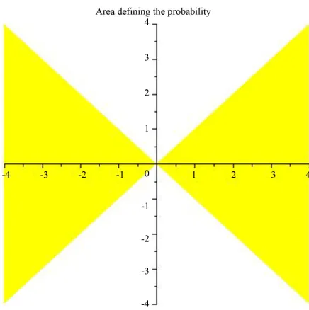
We now calculate the following probability illustrated in the following diagram Figure 1, where the horizontal axis gives values of ˆ1 while the vertical gives values of ˆ1.





















1 1 1 1 1 1

1 1 1 1

ˆ

, 0, 0

ˆ _, ˆ _0, ₀

P P

P

     

   

    

ˆ ˆ

    

    

   

  

 

The result is stated in the following Theorem. Theorem

Under the SVSM estimation procedure we have the following probability:

[image:2.595.314.532.496.715.2]

When ρ > 0

Figure 1. Area defining the probability.

(3)





   

2

0 2

1 1 1 1 1

0

2

ˆ _d _d

P g r f r r g r f r r g r



  



  

_



_



_

_{f r r}_d

For ρ < 0





   

2

0 2

1 1 1 1 1

0

2

ˆ ˆ _d _d _d

P h r f r r h r f r r h r f



 

 

 

 

_



_



_

r r

where

 





2 2

2

1

1 2

g r   r  

 

 





 _ 

  _ _

 _  _   

 

  _ _,

2 2

1 1

2

h r r    

 

 _   _

  

    

  

  

   

 





2

1 ₂ 2 1 2

 

1 1

exp 2 2π

f r r  

 

 

 _   _

  and





2

2 ₂ 2 1

1 1

exp 2 2π

f r r  

 

 

 _   _

 2 

Proof: See Appendix

3. Statistical Analysis

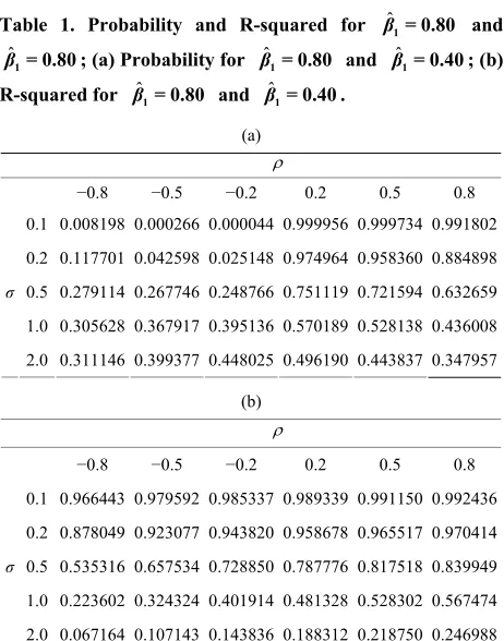
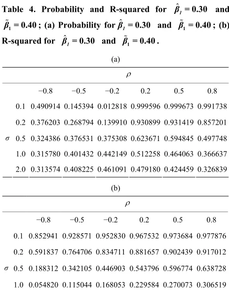
The results show that if the regression was a high R2

and if the two variables are positively correlated, then this procedure leads to a high probability that ˆ1 exceeds 1 not just when ˆ1 exceeds 1, but even when

1 ˆ

 is less than 1 (see Tables 3-5). In the case when

R2_{is low or when the returns are negatively correlated,}

the methodology is less successful. To illustrate our calculations, we carried out some nu-

merical calculations; we calculated the probability that 1

ˆ

 exceeds 1 for different values of σ and ρ; we also computed the R2 _{of the regression. The values of}_σ_were

0.1, 0.2, 0.5, 1.0, and 2.0 whilst the values of ρ were −0.8,

−0.5, −0.2, 0.2, 0.5 and 0.8. Different combinations ofˆ1 and1 were used, namely (0.8, 0.4), (0.5, 0.4), (0.4, 0.4), (0.3, 0.4), and (0.1, 0.4). The output constitutes Tables 1-5.

4. Empirical Examples

For illustrative purposes, we use six Fama-French style based portfolios formed on size and book-to-market1_.

[image:3.595.47.502.80.275.2]

These are: Small Growth (SG), Small Neutral (SN), Small Value (SV), Big Growth (BG), Big Neutral (BN), Big Value (BV). There are two return factors, the first, SMB (Small Minus Big) is the return difference between the average of three small portfolios and the average of three large portfolios, Likewise, the second factor, HML (High Minus Low) is the return difference between the average of two value portfolios and the average of two growth portfolios.

Table 1. Probability and R-squared for and ; (a) Probability for and ; (b)

R-squared for and .

ˆ

β1= 0.80 ˆ

β1= 0.40 ˆ

β1= 0.80 βˆ1= 0.80

ˆ

β1= 0.40 ˆ

β1= 0.80

(a)



−0.8 −0.5 −0.2 0.2 0.5 0.8

0.1 0.008198 0.000266 0.000044 0.999956 0.999734 0.991802

0.2 0.117701 0.042598 0.025148 0.974964 0.958360 0.884898

0.5 0.279114 0.267746 0.248766 0.751119 0.721594 0.632659

1.0 0.305628 0.367917 0.395136 0.570189 0.528138 0.436008

σ

2.0 0.311146 0.399377 0.448025 0.496190 0.443837 0.347957

We choose two different sample periods, where SMB and HML are either positively or negatively correlated. Table 6 lists the regression results for the period from 1935 Jan to 1954 Dec, where SMB and HML are positively correlated with ρ= 0.529; Table 7 lists the regression results for the period from 1992 Jan to 2011 Dec with ρ = −0.348. In our sequential variable selection model, SMB is variable 1 and HML is variable 2. ˆ1 is the estimated coefficient from the univariate regression (b)



−0.8 −0.5 −0.2 0.2 0.5 0.8

0.1 0.966443 0.979592 0.985337 0.989339 0.991150 0.992436

0.2 0.878049 0.923077 0.943820 0.958678 0.965517 0.970414

0.5 0.535316 0.657534 0.728850 0.787776 0.817518 0.839949

1.0 0.223602 0.324324 0.401914 0.481328 0.528302 0.567474

σ

2.0 0.067164 0.107143 0.143836 0.188312 0.218750 0.246988

1_{The stocks are ranked based on two independent criteria: size (market}

[image:3.595.57.288.435.729.2]

(4)

[image:4.595.306.538.84.379.2]

Table 2. Probability and R-squared for and ; (a) Probability for and (b)

ˆ

β1= 0.50

β1= 0.40

β1= 0.40 βˆ1= 0.50

β1= 0.40 ˆ

β1= 0.50

(a)



−0.8 −0.5 −0.2 0.2 0.5 0.8

0.1 0.041297 0.001569 0.000057 0.999956 0.999734 0.991802

0.2 0.196088 0.089434 0.039651 0.971446 0.956407 0.881919

0.5 0.292002 0.318466 0.308932 0.690551 0.660531 0.563587

1.0 0.307585 0.385128 0.421232 0.536673 0.490127 0.393426

σ

2.0 0.311519 0.404026 0.455544 0.485904 0.431795 0.334440

(b)



−0.8 −0.5 −0.2 0.2 0.5 0.8

0.1 0.900000 0.954545 0.970588 0.980000 0.983871 0.986486

0.2 0.692308 0.840000 0.891892 0.924528 0.938462 0.948052

0.5 0.264706 0.456522 0.568966 0.662162 0.709302 0.744898

1.0 0.082569 0.173554 0.248120 0.328859 0.378882 0.421965

σ

[image:4.595.56.289.84.420.2]

2.0 0.022005 0.049881 0.076212 0.109131 0.132321 0.154334

β1= 0.40

β1= 0.40 β1= 0.40

β1= 0.40

(a)



−0.8 −0.5 −0.2 0.2 0.5 0.8

0.1 0.196464 0.021743 0.000680 0.999950 0.999733 0.991801

0.2 0.273772 0.156281 0.070600 0.961037 0.950293 0.875036

0.5 0.305567 0.345069 0.339541 0.659712 0.630060 0.532287

1.0 0.310969 0.392804 0.431375 0.524599 0.477063 0.379741

σ

2.0 0.312364 0.406016 0.458267 0.482522 0.428049 0.330487

(b)



−0.8 −0.5 −0.2 0.2 0.5 0.8

0.1 0.864865 0.941176 0.962406 0.974619 0.979592 0.982935

0.2 0.615385 0.800000 0.864865 0.905660 0.923077 0.935065

0.5 0.203822 0.390244 0.505929 0.605678 0.657534 0.697337

1.0 0.060150 0.137931 0.203822 0.277457 0.324324 0.365482

σ

[image:4.595.307.537.406.734.2]

2.0 0.015748 0.038462 0.060150 0.087591 0.107143 0.125874

ˆ 1

β = 0.30

β1= 0.40

β1= 0.40 βˆ1= 0.30

β1= 0.40 ˆ

1

β = 0.30

(a)



−0.8 −0.5 −0.2 0.2 0.5 0.8

0.1 0.490914 0.145394 0.012818 0.999596 0.999673 0.991738

0.2 0.376203 0.268794 0.139910 0.930899 0.931419 0.857201

0.5 0.324386 0.376531 0.375308 0.623671 0.594845 0.497748

1.0 0.315780 0.401432 0.442149 0.512258 0.464063 0.366637

σ

2.0 0.313574 0.408225 0.461091 0.479180 0.424459 0.326839

(b)



−0.8 −0.5 −0.2 0.2 0.5 0.8

0.1 0.852941 0.928571 0.952830 0.967532 0.973684 0.977876

0.2 0.591837 0.764706 0.834711 0.881657 0.902439 0.917012

0.5 0.188312 0.342105 0.446903 0.543796 0.596774 0.638728

1.0 0.054820 0.115044 0.168053 0.229584 0.270073 0.306519

σ

2.0 0.014293 0.031477 0.048072 0.069335 0.084668 0.099505

ˆ 1

β = 0.10

β1= 0.40

β1= 0.40 βˆ1= 0.10

β1= 0.40 ˆ

1

β = 0.10

(a)



−0.8 −0.5 −0.2 0.2 0.5 0.8

0.1 0.815601 0.751707 0.393672 0.918113 0.972403 0.976545

0.2 0.599814 0.586064 0.431205 0.740597 0.794515 0.747375

0.5 0.376591 0.451091 0.458812 0.539563 0.514171 0.423813

1.0 0.329611 0.421336 0.465250 0.487285 0.438907 0.342919

σ

2.0 0.317082 0.413286 0.467019 0.472654 0.417802 0.320514

(b)



−0.8 −0.5 −0.2 0.2 0.5 0.8

0.1 0.913793 0.928571 0.939024 0.948980 0.954545 0.959016

0.2 0.726027 0.764706 0.793814 0.823009 0.840000 0.854015

0.5 0.297753 0.342105 0.381188 0.426606 0.456522 0.483471

1.0 0.095841 0.115044 0.133449 0.156830 0.173554 0.189627

σ

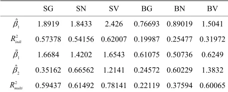
[image:4.595.56.288.417.728.2]

(5)

[image:5.595.57.286.101.194.2]

Table 6. Regression results for six portfolios when ρ = 0.529.

SG SN SV BG BN BV

1 ˆ

 1.8919 1.8433 2.426 0.76693 0.89019 1.5041 2

indi

R 0.57378 0.54156 0.62007 0.19987 0.25477 0.31972

1

 _{1.6684 1.4202 1.6543} _{0.61075 0.50736} _0.6249

2 ˆ

 0.35162 0.66562 1.2141 0.24572 0.60229 1.3832 2

multi

R

[image:5.595.56.287.233.328.2]

0.59437 0.61492 0.78141 0.22119 0.37594 0.60065

Table 7. Regression results for six portfolios when ρ = −0.348.

SG SN SV BG BN BV

1 ˆ

 1.4183 0.93986 0.90215 0.18208 0.047672 0.030638 2

indi

R 0.50081 0.39152 0.32264 0.02081 0.001394 0.000484

1

 _{1.2584 1.0111 1.0787 0.027752 0.11295 0.20748}

2 ˆ

 −0.47902 0.21332 0.5288 −0.46232 0.19554 0.52974 2

multi

R 0.5471 0.40787 0.41246 0.12952 0.020397 0.11761

of y on SMB; 1 is the coefficient on SMB from the multiple regression of y on SMB and HML; ˆ2 is the coefficient on HML and calculated by regressing the residual of y on SMB upon the residual of HML on SMB.

We are interested in the following question. Under what circumstances will there be a larger estimated ex- posure ˆ1 than1? The results show that when the two variables are positively correlated as in Table 6, this procedure always generates higher ˆ1 than 1. When the two variables are negatively correlated as in Table 7, we identify higher ˆ1 than 1 only for two portfolios SG and BG; for the other four portfolios, ˆ1 is lower than

1

 _{. Therefore comparing the two different cases, we find}

out that the methodology is more successful when ρ is positively correlated. This confirms our finding in section 3.

5. Conclusions

Bayesian methods are notoriously difficult to implement and practitioners often use tricks to allow their models to

reflect their beliefs. We discuss such a procedure, and show analytically conditions when it will work. The particular procedure we discuss is used by practitioners to build factor models. We are interested in the variable selection methodologies that are used to give a particular returns model a particular style and nature. For example, in the context of global models one may wish the model to depend more/less upon domestic factors such as country indices rather than, say, global factors such as currency or world equity/bond markets. The method we discuss allows for favorable selection of a variable by spe- cifying the order in which variables enter a regression. We strip the problem down to its bare essentials by considering bivariate situations. We evaluate these conditions using numerical integration and further confirm their relevance by looking at an empirical example. The examples used US equity data over 20 years period. These illustrate the efficacy of the procedure.

REFERENCES

[1] P. Jorion, “Bayes-Stein Estimation for Portfolio Analy-sis,” Journal of Financial and Quantitative Analysis, Vol. 21, No. 3, 1986, pp. 279-292. doi:10.2307/2331042 [2] F. Black and R. Litterman, “Global Asset Allocation with

Equities, Bonds and Currencies,” Goldman Sachs and Co., New York, 1991.

https://faculty.fuqua.duke.edu/~charvey/Teaching/BA453 _2006/Black_Litterman_GAA_1991.pdf

[3] F. Black, and R. Litterman, “Global Portfolio Optimiza-tion,” Financial Analysts Journal, Vol. 48, No. 5, 1992, pp. 28-43. doi:10.2469/faj.v48.n5.28

[4] S. Satchell and A. Scowcroft, “A Demystification of the Black-Litterman Model: Managing Quantitative and Tra-ditional Portfolio Construction,” Journal of Asset Man-agement, Vol. 1, No. 2, 2000, pp. 138-150.

doi:10.1057/palgrave.jam.2240011

(6)

Appendix: Proof of Theorem

[image:6.595.67.536.89.480.2]

Diagrammatically we need to calculate the two areas in Figure 1 on either side of the origin.





 

0

diagram , d d

r

RHS f r s s r

 



_{ }



diagram



0

 

, d d r

r

LHS f r s s r

 



_{ }

Now

 

,

 

1

 

f r s  f s r f r

where





2 2 2 ₂ ~ , 1 s r N r   



 

  

 

and



2



1 2,

r N   

First we shall calculate RHS.

 

1

 

0

d d

r

RHS f s r s f r r

        

 

Transforming from s to ω,







2



2

1

s  s r  

      we have 2 d d , 1

s  

   giving  

 

2 2 2 2 2 1 2 1 0 ₁ 2 1

e d d

2π r

RHS f r r

 _                         



For





2 2 2

2 2

1 1

0 r  2 0 2r    

            

 

2 2 2 2 2 2 2

2 ₂ 2

2 2

1 1

2

2 2

1 1

0 ₁ 2 ₁

2 2

1 1

e d d e d d

2π 2π

r r

RHS f r r f r r

 _  _                _                                   



Letting

 





2 2 2 2 2 1 2

2 2 2

2 1

2

1 1

e d 1 2

2π

r

g r r

 _                   _    _ _   _  _        _ _



_

where

 

x is the cumulative distribution function of the standard normal distribution we have:

   

2 2 2 1 1 0 2 d

RHS g r f r r g r f r r







_



_

d

Having completed the calculation of RHS, we now turn to LHS.

 

   

0 0

1

, d d d

r

LHS f r s s r g r f r r

  



_{ }



_

We can make further simplifications depending upon the sign of ρ.

For ρ > 0





   

2

1 1 1

0 0 1 2 ˆ _d d

P g r f r r

1 d

g r f r r g r f r r

         



 where

 





2

1 ₂ 2 1

1 1

exp 2 2π

f r r  

 

 

 _   _

 2 

When ρ< 0 rewrite using –ρ and then let ρ > 0. Thus we now have:





1 2 2

1 2 1 1 1 ~ , 1 1 r N s       _ _ _     _ _ __     _ _ _ __   _  _ __





2 2 2 ₂ ~ , 1 s r N r   



 

  

  

 



2



1 2

~ ,

r N   

Now,

 

2

 

0

d d r

r

RHS f s r f r s r

 



_{ }

and again transforming from s to ω,



2



2

1

s  s r  





    with

2

d d

1 s  



(7)

 

2 2

2

2 2

1

2 2

0 ₁

2

1

e d d

2π r

RHS f r r

  

 

 



 



 

 

 

 



 

 



Letting

 









2 2

2

2 2

1

2 2

2 1

2

2 2

1 1

1 _e _d ₂

2π

1 1

2 r

h r r

r

 



 

 

  

 

 

  



 

 

 

_ _   _

  

      

  

  

 _   _ 

   

    

   

   





    

   

2 0

d

RHS h r f r r





_

For



2



2

2 r 1

r   

 

       

and

   

2

0

2

0 2

2 2

2 d

d d

LHS h r f r r

h r f r r h r f r r



 

 



 



Thus for ρ < 0.





   

2

1 1 2

0

0 2

2 2

2

ˆ ˆ _d

d d

P h r f r r

h r f r r h r f r r



  



 

 

 



where

 





2

2 ₂ 2 1

1 1

exp 2 2π

f r r  

 

 

 _   _