Munich Personal RePEc Archive
Periodic autoregressive stochastic
volatility
Aknouche, Abdelhakim
University of Science and Technology Houari Boumediene, Qassim
University
1 June 2013
Online at
https://mpra.ub.uni-muenchen.de/83083/
Periodic autoregressive stochastic volatility
Abdelhakim Aknouche
yDecember 2, 2017
Abstract
This paper proposes a stochastic volatility model (P AR-SV) in which the log-volatility follows a
…rst-order periodic autoregression. This model aims at representing time series with volatility displaying
a stochastic periodic dynamic structure, and may then be seen as an alternative to the familiar periodic
GARCH process. The probabilistic structure of the proposedP AR-SV model such as periodic
station-arity and autocovariance structure are …rst studied. Then, parameter estimation is examined through the
quasi-maximum likelihood (QM L) method where the likelihood is evaluated using the prediction error
de-composition approach and Kalman …ltering. In addition, a BayesianM CM Cmethod is also considered,
where the posteriors are given from conjugate priors using the Gibbs sampler in which the augmented
volatilities are sampled from the Griddy Gibbs technique in a single-move way. As a-by-product, period
selection for theP AR-SV is carried out using the (conditional) Deviance Information Criterion (DIC).
A simulation study is undertaken to assess the performances of the QM Land Bayesian Griddy Gibbs
estimates in …nite samples while applications of Bayesian P AR-SV modeling to daily, quarterly and
monthlyS&P 500 returns are considered.
Keywords and phrases: Periodic stochastic volatility, periodic autoregression, QM Lvia prediction
error decomposition and Kalman …ltering, Bayesian Griddy Gibbs sampler, single-move approach,DIC.
Mathematics Subject Classi…cation: AMS 2000 Primary 62M10; Secondary 60F99
Proposed running head: Periodic AR Stochastic volatility.
1. Introduction
Over the past three decades, stochastic volatility (SV) models introduced by Taylor (1982)have played an
important role in modelling …nancial time series which are characterized by a time-varying volatility feature.
Faculty of Mathematics, University of Science and Technology Houari Boumediene, Algiers, Algeria, e-mail: [email protected].
yThis is a long version of the paper Aknouche (2017)[Periodic autoregressive stochastic volatility. Statistical Inference
This class of models is often viewed as a better formal alternative to ARCH-type models because the
volatility is itself driven by an exogenous innovation, a fact that is consistent with …nance theory, although it
makes the model relatively more di¢cult to estimate. Several extensions of the originalSV formulation have
been proposed in the literature to account for further volatility features such as long memory, simultaneous
dependence, excess kurtosis, leverage e¤ect and change in regime (e.g. Harvey et al, 1994; Ghysels et al,
1996; Breidt,1997; Breidt et al,1998; So et al,1998; Chib etal,2002; Carvalho and Lopes,2007; Omori et
al, 2007; Nakajima and Omori,2009). However, it seems that most of the proposed formulations have been
devoted to time-invariant volatility parameters and hence they could not meaningfully explain time series
whose volatility structure changes over time, in particular volatility displaying a stochastic periodic pattern
that cannot be accounted for by time-invariantSV-type models.
In order to describe periodicity in the volatility, Tsiakas(2006)proposed various interesting and
parsimo-nious time-varying stochastic volatility models in which the volatility parameters are expressed as
determin-istic periodic functions of time with appropriate exogenous variables. The proposed models called "periodic
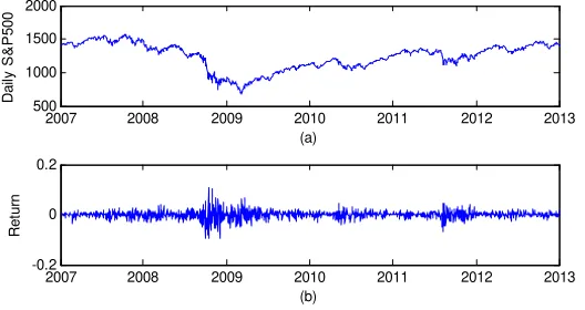
stochastic volatility" (P SV) have been successfully applied to model the evolution of dailyS&P 500returns.
This is an evidence that the periodically changing structure may characterize time series volatility. However,
the P SV formulations are by de…nition especially well adapted to a kind of deterministic periodicity in
the second moment and hence they might neglect a possible stochastic periodicity in these moments (see
e.g. Hylleberg et al (1990)and Ghysels and Osborn (2001) for the di¤erence between deterministic and
stochastic periodicity). A complementary approach which seems to be appropriate in capturing stochastic
periodicity in the volatility is to consider a linear time-invariant representation for the volatility equation
involving seasonal lags, leading to a seasonal SV speci…cation (see e.g. Ghysels et al, 1996). However,
because of the time-invariance of the volatility parameters, the seasonal SV model may be too restrictive
in representing periodicity and a model with periodic time-varying parameters seems to be more relevant.
Indeed, as pointed out by Bollerslev and Ghysels(1996, p. 140)many …nancial time series encountered in
practice are such that neglecting periodic time-variation in the corresponding volatility equation give rise
to a loss in forecast e¢ciency, which is more severe in the GARCH model than in linear ARM A. This
has motivated Bollerslev and Ghysels (1996)to propose the periodicGARCH (P GARCH) formulation in
which the parameters vary periodically over time in order to capture the stochastic periodicity pattern in
the conditional second moment. At present theP GARCH model is among the most important models for
describing periodic time series volatility (see e.g. Bollerslev and Ghysels,1996; Taylor,2006; Koopman etal,
2007; Osborn etal,2008; Regnard and Zakoïan,2011; Sigauke and Chikobvu, 2011; Aknouche and Al-Eid,
2012). However, despite the recognized relevance of the P GARCH model, an alternative periodicSV for
stochastic periodicity is in fact needed for many reasons. First, it is well known that an SV-like model is
observed process which constitutes a serious limitation. Second, because of the proliferation of parameters,
theP-GARCHinduces a supplementary di¢culty in the estimation stage due to the positivity restriction on
the parameters. In many instances, this constraint may be violated as some volatility parameter estimates
would be negative. Third, compared toSV-type models, the probability structure of P GARCH models is
relatively more complex to obtain (Aknouche and Bibi,2009). Finally, theP AR-SVS easily allows to simple
multivariate generalizations.
In this paper we propose to model stochastic periodicity in the volatility through a model that generalizes
the standardSV equation so that the parameters vary periodically over time. Thus, in the proposed model
termedperiodic autoregressive stochastic volatility (P AR-SVS) the log-volatility process follows a …rst-order
periodic autoregression and may be generalized so as to have any linear periodic representation. This model
may be seen as an extension of the models of Tsiakas(2006)to include periodic feature in the autoregressive
dynamic of the log-volatility equation. The structure and probability properties of the proposed model such as
periodic stationarity, autocovariance structure and relationship with multivariate stochastic volatility models
are …rst studied. In particular, periodicARM A(P ARM A)representations for the logarithm of the squared
P AR-SVS process are proposed. Then, parameter estimation is conducted via the quasi-maximum likelihood
(QM L) method, properties of which are discussed. In addition, Bayesian estimation approach using Markov
Chains Monte Carlo(M CM C)techniques is also considered. Speci…cally, a Gibbs sampler is used to estimate
the joint posterior distribution of the parameters and the augmented volatility while calling for the Griddy
Gibbs procedure when estimating the conditional posterior distribution of the augmented parameters. On
the other hand, selection of the period of theP AR-SVS model is carried out using the (conditional) Deviance
Information Criterion (DIC). Simulation experiments are undertaken to assess …nite-sample performances
of theQM LE and the Bayesian Griddy Gibbs methods. Moreover, empirical applications to modeling series
of daily, quarterly and monthly S&P 500 returns are conducted in order to appreciate the usefulness of
the proposedP AR-SVS model. In the particular daily return case, a variant of the P AR-SVS model with
missing values, dealing with the "day-of-the-week" e¤ect is applied.
The rest of this paper proceeds as follows. Section 2 proposes the P AR-SVS model and studies its
main probabilistic properties. In Section 3, the quasi-maximum likelihood method via prediction error
decomposition and Kalman …ltering is adopted. Moreover, a single-move Bayesian approach by means of the
Griddy Gibbs (BGG) sampler is proposed. In particular, some M CM C diagnostic tools are presented and
period selection in P AR-SVS models is carried out using theDIC. Through a simulation study, Section 4
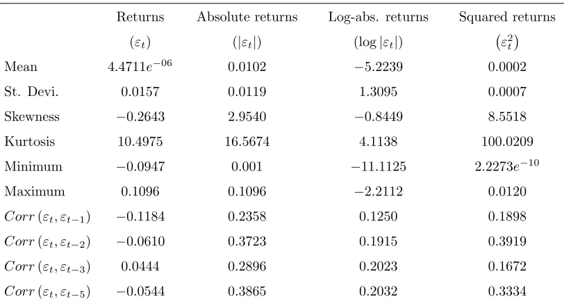
examines the behavior of the QM L andBGGmethods in …nite samples. Section 5 applies the P AR-SVS
speci…cation to model daily, quarterly and monthly S&P 500 returns using the Bayesian Griddy Gibbs
2. The
P AR
-
SV
Sand its main probabilistic properties
In this paper, we say that a stochastic processf"t; t2Zghas a periodic autoregressive stochastic volatility
representation with periodS (P AR-SVS in short) if it is given by 8
< :
"t=
p
ht t
log (ht) = t+ tlog (ht 1) + tet
, t2Z; (2:1a)
where the parameters t; t;and tareS-periodic overt(i.e. t= t+Sn8n2Zand so on) and the period
S 1 is the smallest positive integer verifying the latter relationship. The sequence of random vectors
f( t; et); t2Zgis assumed to be independent and identically distributed (iidin short) with mean(0;0)0 and
covariance matrixI2(I2stands for the identity matrix of dimension2). We have called model(2:1a)periodic
autoregressive stochastic volatility rather than shortlyperiodic stochastic volatility because the log-volatility
is rather driven by a …rst-order periodic autoregression and also in order to make distinction between model
(2:1a)and the periodic stochastic volatility (P SV) model proposed by Tsiakas (2006). In fact, the P AR
-SVS model(2:1a)may be generalized so thathtsatis…es any stable periodicARM A(henceforth P ARM A)
representation.
Remark 2.1 While the P AR-SV allows for a periodic-time varying dependence structure, it only ex-presses dependence between successive times but not between times distanced by a multiple of the periodS
such as time-invariant seasonal models. A useful periodicSV model which takes into account of successive
de-pendence,S-lagged dependence and periodic time-varying dependence would be the following multiplicative
SP AR-SV (1;0) (1;0)representation
yt =
p
ht t
log (ht) = t+ tlog (ht 1) + tlog (ht S) t tlog (ht S 1) + et;
where t; tand tareS-periodic over time. This representation has been proposed in the context of linear
models by Basawa etal (2004)who discussed the properties and inference of the model. However, the latter
SP AR-SV(1;0)(1;0)is more di¢cult to estimate using quasi-maximum likelihood and Bayesian approaches
(see Section 3) because of its nonlinear form with respect to the parameters, and its non …rst-order Markov
property.
Note that when t= 0, model(2:1a)reduces to Tsiakas’s(2006)model if we take tto be an appropriate
deterministic periodic function of time. In that case, the e¤ect of any current shock in the innovationetonly
in‡uences the present volatility and does not a¤ect its future evolution. This is the case of what is called
deterministic periodicity (Hylleberg etal,1990). If, in contrast, t6= 0for somet, the log-volatility equation
involves lagged values of the log-volatility process. Therefore, the log-volatility consists at any time of an
depending on the stability of the log-volatility equation (see the periodic stationarity condition(2:5)below).
This case is commonly named stochastic periodicity in the volatility.
It should be noted that although ht is conventionally called volatility, it is not the conditional variance
of the observed process given its past information in the familiar sense as in ARCH-type models. This is
because ht is insteadFt-measurable and so E "2t=Ft 1 = E(ht=Ft 1) 6= ht, where Ft is the -Algebra
generated byf"u; u tg. Nevertheless,E(ht) =E "2t andE "2t=ht =ht as in theARCH-type case.
To emphasize the periodicity of the model, let t=nS+v forn2Zand1 v S. Then model(2:1a)
may be written as follows
8 < :
"nS+v=
p
hnS+v nS+v
log (hnS+v) = v+ vlog (hnS+v 1) + venS+v
,n2Z; 1 v S; (2:1b)
where by season v (1 v S) we mean the channel f:::; v S; v; v+S; v+ 2S; :::g with corresponding
parameters v; v and v.
From(2:1b)the log-volatility appears to be a Markov chain, which is not homogeneous as in time-invariant
stochastic volatility models, but is rather periodically homogeneous due to the periodic time-variation of
parameters. This may relatively complicate studying the probabilistic structure of the P AR-SVS model.
As is common in periodic time varying modeling, a routine approach is to write (2:1b)as a time-invariant
multivariate SV model by embedding seasons v, 1 v S (see e.g. Gladyshev, 1961 and Tiao and
Grupe, 1980for periodic linear models) and then studying the property of this latter (e.g. Smith, 2010).
More precisely, de…ne the S-variate sequences fHn; n2Zg, f"n; n2Zg by Hn = (hnS+1; :::; hnS+S)0 and
"n= ("nS+1; :::; "nS+S)0. Then model(2:1b)may be cast in the following multivariateSV form 8
< :
"n=diag H
1 2
n n
logHn =BlogHn 1+ n
, n2Z; (2:2)
where n= nS+1; :::; nS+S
0
,diag(a)stands for the diagonal matrix formed by the entries of the vector
ain the given order. The notations H
1 2
n andlogHn denote the S-vectors de…ned respectively byH
1 2
n (v) = p
hnS+v andlogHn(v) = log (hnS+v)(1 v S). The matricesB and n in (2:2) are given by
B=
0 B B B B B B B @
0 : : : 0 1
0 : : : 0 2 1
..
. ... ... ...
0 : : : 0
S Q v=1 S v
1 C C C C C C C A
S S
; n=
0 B B B B B B B @
nS+1
2 nS+1+ nS+2 ..
.
S P k=1
S kQ 1
v=0 S v nS+k
1 C C C C C C C A
S 1
;
with nS+v= v+ venS+v (1 v S).
However, this approach has the main drawback that available methods for analyzing multivariate SV
on model (2:1). Thus, studying probabilistic and statistical properties of model (2:1) directly may be
simpler and better than studying them through model(2:2). This suggests that periodic stochastic volatility
modelling cannot be trivially deduced from existing multivariateSV analysis. In the sequel, we study the
structure of model(2:1)using mainly the direct approach.
Throughout this paper, we frequently use solutions of the following ordinary di¤erence equation
ut=at+btut 1; t2Z; (2:3a)
withS-periodic coe¢cientsatandbt. Recall that the unique solution of(2:3a)is given, under the requirement
that
S Q v=1
bv <1, by
unS+v= 1
S Y
v=1
bv
! 1S 1
X
j=0
jY1
i=0
bv iav j, 1 v S; n2Z. (2:3b)
Before studying the probabilistic properties of model (2:1), it is useful to recall some probability
proper-ties related to periodically time-varying stochastic di¤erence equations like strict periodic stationarity and
periodic ergodicity. A real-valued stochastic process fYt; t2Zg de…ned on a probability space ( ;F; P)
is said to bestrictly periodically stationary (henceforth s:p:s:) with periodS 1 if its in…nite-dimensional
distribution is invariant under a shift multiple ofS for all channelv(1 v S), i.e. the probability
distrib-ution of(:::; Yv; Yv+1; Yv+2; :::)is the same as that of(:::; Yv+hS; Yv+1+hS; Yv+2+hS; :::)for all1 v S and
allh2Z, where S is the smallest positive integer verifying the latter property. For instance, the simplest
s:p:s:process is a sequencefut; t2Zgof independent and periodically distributed random variables
(hence-forth ipd), i.e. fut; t2Zg is independent and ut has the same distribution asut+nS for all t; n2Z. Thus
a s:p:s: process with S = 1 is a strictly stationary one and anidp sequence withS = 1reduces to an iid
sequence. Like the ergodic theorem for strictly stationary processes, the periodic ergodic theorem for strictly
periodically stationary sequences can be stated as follows. If fYt; t2Zg iss:p:s: and if f is a measurable
function fromRZto Rsuch thatE(f(:::; Yt S; Yt; Yt+S; :::))<1for allt2Z, then
1 n
n 1
X
k=0
f :::Yv+(k 1)S; Yv+kS; Yv+(k+1)S; :::
a:s:
!
n!1Yv,81 v S;
for some random variableYv. WhenfYnS+v; n2Zgsatis…es for all channel1 v Sa certainirreducibility
property calledperiodic ergodicity, which roughly means thatfYnS+v; n2Zgmay reach any nonP-negligible
subclass of the state space for all1 v S, then the limiting random variableYv is almost surely constant
and then
Yv =E(f(:::; Yv S; Yv; Yv+S; :::)); (1 v S); a:s:
To de…ne periodic ergodicity, let T : RZ ! RZ denote the shift transformation de…ned for any xv =
of T: TS =T T ::: T, S times. Thus, fY
t; t2Zg is s:p:s: if and only ifTS preserves the probability
measure PYv for all 1 v S (PYv being the image measure of P by the process fYnS+v; n2Zg). A
Borel setCv RZof the form Cv = xv 2RZ:xv= (:::; xv; xv+1; xv+2; :::) is said to beS-invariant along the channel v (1 v S) ifT S(C
v) =Cv, where T S(Cv) = xv 2RZ:TSxv2Cv . A s:p:s: process
fYt; t2Zg is said to be periodically ergodic if for all 1 v S, P((:::; Yv; Yv+1; Yv+2; :::)2Cv) = 0 or
1, for all S-invariant Borel set Cv over channel v. Similarly to strict periodic stationarity, the simplest
periodically ergodic process is a sequence of ipd random variables. Like strict stationarity and ergodicity
(see e.g. Billingsley,1995, Theorem36:4), strict periodic stationarity and periodic ergodicity are preserved
under certain transformations. Indeed, iffYt; t2Zg iss:p:s:and periodically ergodic and if fZt; t2Zg is
given byZt=ft(:::; Yt; Yt+1; Yt+2; :::), whereft is a function fromRZ intoRwhich is measurable, periodic
over t with period S (ft = ft+nS for alln and t), and possibly depending on S-periodically time-varying
parameters, thenfZt; t2Zgis alsos:p:s:and periodically ergodic. Thus a sequence ofipdrandom variables
may be seen as a "building-block" for the class ofs:p:s:and periodically ergodic processes.
Now, we have the following result which provides a necessary and su¢cient condition for strict periodic
stationarity and periodic ergodicity of model(2:1).
Theorem 2.1 (Strict periodic stationarity)
The P AR-SVS equation given by (2:1)admits a unique (nonanticipative) strictly periodically stationary
and periodically ergodic solution given for n2Z and 1 v S by
"nS+v= nS+vexp
8 > > > < > > > :
1 2
0 B B B @
PS 1
j=0
jQ1
i=0 v i v j
1
S Q v=1 v
+
1
X
j=0
jY1
i=0
v i v jenS+v j 1 C C C A
9 > > > = > > > ;
; (2:4)
where the series in (2:4) converges almost surely, if and only if,
S Y
v=1
v <1: (2:5)
Proof The result obviously follows from standard linear periodic autoregression (P AR) theory while using(2:3)(see e.g. Aknouche and Bibi,2009). So, details are omitted.
From(2:5)we see that the monodromy coe¢cient QS
v=1 v
is the analog of the persistent parameter in the
case of time-invariantSV and standard GARCH models.
Other properties such as periodic geometric ergodicity and strong mixing are obvious. Let …rst say
that a strictly periodically stationary stochastic process f"t; t2Zg is said to be geometrically periodically
ergodic if and only if the corresponding multivariate strictly stationary process f"t; t2Zg given by "n =
("nS+1; :::; "nS+S)0 is geometrically ergodic in the classical sense (see e.g. Meyn and Tweedie,2009 for the
de…nition of geometric ergodicity). Similarly, f"t; t2Zg is said to beperiodically -mixing if and only if
Theorem 2.2 (Geometric periodic ergodicity)
Under the condition
S Q v=1 v
<1, the process f"t; t2Zg de…ned by (2:1) is geometrically periodically
ergodic and hence is periodically -mixing.
Proof The result follows from geometric ergodicity of the vector autoregressionflogHn; n2Zggiven by
(2:2), which may be easily established using Meyn and Tweedie’s(2009)results (see also Davis and Mikosch,
2009).
Given the form of the strictly periodically stationary solution (2:4), it is easy to give its second-order
properties. Assume …rst the following conditions hold
E Q1
j=0
v;j !
= Q1
j=0
E( v;j) for all1 v S; (2:6a)
1
Q j=0
v;j < 1 for all1 v S; (2:6b)
where
v;j = exp
jY1
i=0
v i v jev j !
and v;j=E( v;j):
As pointed out by an Associate Editor, equality (2:6a)is not always satis…ed for any independent
se-quencef j; j2Ng and one can exhibit examples of independent sequences for which(2:6a)is not ful…lled.
Nevertheless, from thedominated convergence theorem, a su¢cient condition for(2:6a)to be satis…ed is that
n Y
j=1
v;j Wv a:s:for alln2N; (2:6c)
for some integrable random variableWv (1 v S).
Thus under (2:5) and(2:6) the following result provides su¢cient conditions for model (2:1) to have a
unique strictly periodically stationary solution with …nite second moment.
Theorem 2.3 (Second-order periodic stationarity)
Under conditions (2:5) and (2:6), the series in (2:4) also converges in the mean square sense and the
process given by (2:4)is strictly periodically stationary with E "2
v <1(1 v S).
Proof Routine computation shows that under(2:5)and(2:6) the series in(2:4);
1
X
j=0
jY1
i=0
v i v jenS+v j; 1 v S;
converges in mean square. Moreover, under these conditions, it is clear that f"t; t2Zg given by (2:4) is a
and, while using(2:3),
V ar("nS+v) = E
0 B B B @exp 0 B B B @ PS 1 j=0
jQ1
i=0 v i v j
1
S Q v=1 v
+
1
X
j=0
jY1
i=0
v i v jenS+v j 1 C C C A 1 C C C A = exp 0 B B B @ PS 1 j=0
jQ1
i=0 v i v j
1
S Q v=1 v
1 C C C A 1 Q j=0
v;j; 1 v S: (2:7)
In the case of Gaussian log-volatility innovations fet; t2Zg, (i.e. et N(0;1)) it is also possible to
obtain more explicit results reducing then assumptions of Theorem 2.3. Using the fact that ifX N(0;1)
thenE(exp( X)) = exp(22)for all non-null real constant , we obtain
v;j= exp
1 2
2
v j jY1
i=0 2
v i !
; (2:8)
and condition(2:6b)of …niteness ofQ1j=0 v;j reduces to the periodic stationarity condition(2:5): S Q v=1 v
<
1. Moreover, using(2:8)and(2:3)the variance of the process given by(2:7)may be expressed more explicitly
as follows
V ar("nS+v) = exp
0 B B B @ PS 1 j=0
jQ1
i=0 v i v j
1
S Q v=1 v
1 C C C A 1 Q j=0 exp 1 2 2 v j jY1
i=0 2 v i ! = exp 0 B B B @ PS 1 j=0
jQ1
i=0 v i v j
1
S Q v=1 v
1 C C C Aexp 0 @1 2 1 X j=0
jY1
i=0 2
v i 2v j 1 A = exp 0 B B B @
SP1
j=0
jQ1
i=0 v i v j
1
S Q v=1 v
+1
2
SP1
j=0
jQ1
i=0 2
v i 2v j
1 S Q v=1 2 v 1 C C C
A: (2:9)
For example, the varianceV ar("nS+v)of the process is given respectively, forS= 2andS = 3, by
V ar("2n+1) = exp 1+ 1 2
1 1 2
+1
2
2 1+
2 1 22
1 21
2 2
;
V ar("2n+2) = exp 2+ 2 1
1 1 2
+1
2
2 2+
2 2 21
1 21
2 2
V ar("3n+1) = exp 1
+ 1 3+ 1 3 2
1 1 2 3
+1
2
2
1+ 21 23+ 1 3 22
1 1 2 3
;
V ar("3n+2) = exp 2+ 2 1+ 2 1 3
1 1 2 3
+1
2
2
2+ 2 21+ 2 1 23
1 1 2 3
;
V ar("3n+3) = exp 3
+ 3 2+ 3 2 1
1 1 2 3
+1
2
2
3+ 3 22+ 3 2 21
1 1 2 3
:
Next, the autocovariance function of the squared process "2
t; t2Z is provided. This one is useful in
identifying the model and deriving certain estimation methods such as simple and generalized methods of
moments. Let "2
v (h) =E "2nS+v"2nS+v h E "2nS+v E "2nS+v h .
Theorem 2.4 (Autocovariance structure of "2
t; t2Z )
i) Under (2:5),(2:6)and the conditions Qj1=0 v;j v h;j<1and E 41 <1we have
"2
v (0) = exp
0 B B B @2
SP1
j=0
jQ1
i=0 v i v j
1
S Q v=1 v
1 C C C A 0
@E 41 E
0 @exp 0 @2 1 X
j=h jY1
i=0
v i v jev j 1 A
1 A Q1
j=0 2
v;j 1
A; (2:10a)
"2
v (h) = 0 @E 0 @exp 0 @ h 1 X j=0
jY1
i=0
v i v jev j+ 1 + hY1
i=0 1
v i ! 1
X
j=h jY1
i=0
v i v jev j 1 A 1 A 1 Q j=0
v;j v h;j ! exp 0 B B B @
SP1
j=0
jQ1
i=0 v i v j
+
SP1
j=0
jQ1
i=0 v h i v h j
1
S Q v=1 v
1 C C C
A; h >0: (2:10b)
Proof Using(2:4)direct calculation gives
E "2nS+v"2nS+v h =E
0 @exp 0 @ 1 X j=0
jY1
i=0
v i v jenS+v j+
1
X
j=0
jY1
i=0
v h i v h jenS+v h j 1 A 1 A exp 0 B B B @ PS 1 j=0
jQ1
i=0 v i v j
1
S Q v=1 v
+
PS 1
j=0
jQ1
i=0 v h i v h j
1
S Q v=1 v
1 C C C AE 2
nS+v 2nS+v h ; (2:11)
under …niteness of the latter expectations. When in particular h= 0, combining (2:7) and (2:11) we get
Forh >0, because of the independence structure off t; t2Zgone obtains
E "2nS+v"2nS+v h = exp
0 B B B @
SP1
j=0
jQ1
i=0 v i v j
+
SP1
j=0
jQ1
i=0 v h i v h j
1
S Q v=1 v
1 C C C A E 0 @exp 0 @ h 1 X j=0
jY1
i=0
v i v jev j+
1
X
j=h jY1
i=0
v i v jev j+
1
X
j=0
jY1
i=0
v h i v h jev h j 1 A 1 A = exp 0 B B B @
SP1
j=0
jQ1
i=0 v i v j
+SP1
j=0
jQ1
i=0 v h i v h j
1
S Q v=1 v
1 C C C A E exp
hP1
j=0
jQ1
i=0 v i v j
ev j+ 1 +
hQ1
i=0 1
v i
1
P j=h
jQ1
i=0 v i v j
ev j
!!
;
giving(2:10b).
The S kurtoses Kurt(v) (1 v S) of the P AR-SVS model may be given from (2:9) and (2:10) as
follows
Kurt(v) = E 41
Q1
j=0E exp
jQ1
i=0 v i v j
ev j
2!
Q1
j=0 E exp
jQ1
i=0 v i v j
ev j
2; 1 v S; (2:12)
E 4
1 :
By the Cauchy-Schwartz inequality, this clearly shows that the P AR-SVS model may be characterized
by excess Kurtosis for all channelsf1; :::; Sg. In particular, under the normality assumption on the
innova-tions, the second-order periodic stationarity reduces to(2:6a)and the following conditionsE( 4
1)<1and
S Q v=1 v
<1. So from(2:8), expression(2:12)reduces to
Kurt(v) =E 41 ; 1 v S:
The autocovariance function has also a more explicit form in the case of Gaussian fet; t2Zg.
Corollary 2.1 (Autocovariance structure of "2
t; t2Z under normality offet; t2Zg)
Under the same assumptions of Theorem 2.4 and if fet; t2Zg is Gaussian then,
"2
v (0) = exp
0 @2 1
S Y
v=1
v
! 1S 1
X
j=0
jY1
i=0
v i v j+ 1 S Y
v=1 2
v
! 1S 1
X
j=0
jY1
i=0 2
v i 2v j 1
A E 41 1 ;
"2
v (h) = exp
0 B B B @
SP1
j=0
jQ1
i=0 v i v j
+
SP1
j=0
jQ1
i=0 v h i v h j
1
S Q v=1 v
+
SP1
j=0
jQ1
i=0 2
v i 2v j
1 S Q v=1 2 v 1 C C C A 0 B B B @exp 0 B B B @
SP1
j=0
jQ1
i=0 2
v i 2v j
1 S Q v=1 2 v hY1
i=0 v i 1 C C C A 1 1 C C C
A, h >0: (2:13b)
Proof For Gaussian innovations, we use again the fact that ifX N(0;1)thenE(exp( X)) = exp( 22). Therefore,(2:13a)follows from(2:10a)and(2:9). Forh >0 we have
E "2nS+v"2nS+v h = exp
0 @ 1 S Y v=1 v ! 10
@ SX1
j=0
jY1
i=0
v i v j+ SX1
j=0
jY1
i=0
v h i v h j 1 A
1 A
hQ1
j=0
exp 1
2
jY1
i=0 2
v i 2v j ! 1 Q j=0 exp 0 @1
2 1 +
hY1
i=0 1
v i !2j 1
Y
i=0 2
v i 2v j 1 A:
After tedious but straightforward calculation, the autocovariance function at lagh(h >0) simpli…es for
Gaussian innovations to
"2
v (h) = exp
0 B B B @
SP1
j=0
jQ1
i=0 v i v j
+
SP1
j=0
jQ1
i=0 v h i v h j
1
S Q v=1 v
1 C C C A 2 4exp 0 @ h 1 X j=0
jY1
i=0 2 v i 2 v j 2 1 A exp 0 @ 1 X
j=h jY1
i=0 2
v i 2v j 1 + hY1
i=0 1
v i !21
A exp 0 @ 1 X j=0
jY1
i=0 2
v i 2v j 1 A 3 5: = exp 0 B B B @
SP1
j=0
jQ1
i=0 v i v j
+
SP1
j=0
jQ1
i=0 v h i v h j
1
S Q v=1 v
+
SP1
j=0
jQ1
i=0 2
v i 2v j
1 S Q v=1 2 v 1 C C C A 0 B B B @exp 0 B B B @
SP1
j=0
jQ1
i=0 2
v i 2v j
1 S Q v=1 2 v hY1
i=0 v i 1 C C C A 1 1 C C C A;
which is(2:13b).
It is worth noting that expanding the exponential function in (2:13b) under the periodic stationarity
condition (2:5), the autocovariance function "2
v (h) of the squared process "2t; t2Z has the following
equivalent form ash! 1
"2
v (h) K hY1
i=0
and so "2
v (h)converges geometrically to zero as h! 1, where K is an appropriate real constant.
How-ever, the decreasing of "2
v (h)is not compatible with the recurrence equation that satisfy periodicARM A
(P ARM A) autocovariances and we can conclude that the squared process "2
t; t2Z does not admit a
P ARM Aautocovariance representation.
Nevertheless, the logarithmed squared process log "2
t ; t2Z has in fact a P ARM Aautocovariance
structure. Considering the following notationsYt= log "2t , Xt = loght, ut = log 2t , E log 2t = u
andV ar log 2
t = 2u, we have from(2:1)
Yt=Xt+ut: (2:14)
Theorem 2.5 (P ARM A(1;1) representation of log "2
t ; t2Z )
Under assumption(2:5)and …niteness of 2
uthe processfYt; t2Zghas aP ARM AS(1;1)representation
given by
YnS+v Yv = v YnS+v 1 Yv 1 + nS+v v nS+v 1; 1 v S; t2Z; (2:15a)
where Y
v =E(YnS+v),
v = 8 > > < > > :
1 + 2v 2u+ 2v
q
1 + 2v 2u+ 2v 1 2v 2u+ 2v
2 v 2u
if 2
u6= 0
0 if 2u= 0
, 1 v S;
(2:15b)
and f t; t2Zgis a periodic white noise with periodic variance
2
;v=V ar nS+v = 8 > > < > > :
v 2u v
if
S Q v=1 v6
= 0
0 if QS
v=1 v
= 0
,1 v S: (2:15c)
Proof The second-order structure offXt; t2Zg is given form(2:1) while using(2:3),
X
v =E(XnS+v) = v+E(XnS+v 1) = 1
S Q v=1 v
1S 1
P j=0
jQ1
i=0 v i v j ,
X
v (0) =V ar XnS2 +v =
2
vE XnS2 +v 1 + 2v= 1 S Q v=1
2
v
1S 1
P j=0
jQ1
i=0 2
v i 2v j
X
v (h) =Cov(XnS+v; XnS+v h)
= v Xv 1(h 1);
Therefore, using(2:14)we have
Y
v =E(YnS+v) =E(XnS+v) +E(unS+v) = 1 S Q v=1 v
1S 1
P j=0
jQ1
i=0 v i v j
+ u,
Y
v(0) =V ar(YnS+v) =V ar(XnS+v) + 2u= 1
S Q v=1
2
v
1S 1
P j=0
jQ1
i=0 2
v i 2v j+ 2u
Y
v(h) = Xv(h) = v Xv 1(h 1) = v v 1::: v h+1 Xv h(0)
= v v 1::: v h+1 1
S Q v=1
2
v
1S 1
P j=0
jQ1
i=0 2
v h i 2v h j
; h >0:
Clearly the processfYt; t2Zghas aP ARM Arepresentation since
Y
v(h) = v Yv 1(h 1)for anyh >1:
To identify the parameters of such a representation we use expressions of Y
v(h)for h= 0;1. IffYt; t2Zg
has indeed aP ARM Arepresentation(2:15a)then for all1 v S,
Y
v(0) = v Yv(1) + 2;v(1 + v( v v))
Y
v(1) = v Yv 1(0) v 2;v: (2:15d)
Hence, if 2
u6= 0we have for all1 v S;
1 + v( v v)
v
=
Y
v(0) v Yv(1) v Yv 1(0) Yv(1)
=
Y
v(0) 2v Xv 1(0)
v Xv 1(0) + 2u) v Xv 1(0)
=
Y
v(0) Xv(0) 2v v 2u
=
Y
v(0) Yv(0) 2v 2u v 2u
=
2
v+ 2u v 2u
: (2:15e)
The latter equation admits, for all 1 v S, two solutions one of which is with modulus less than
1 (j vj < 1) and is given by (2:15b). Such a choice clearly ensures that S Q v=1j vj
<1, but is not unique.
Moreover, when
S Q v=1 v6
= 0 using(2:15d), the variance off t; t2Zgis
2
;v = v Y
v 1(0) Yv(1) v
= v
X
v 1(0) + 2u v Yv 1(0)
v
;
If, however, 2
u = 0 the relationship Yv(h) = v Yv 1(h 1) also holds for h = 1 and so the process
fYt; t2Zg is a pure …rst-order periodic autoregression (P AR(1)) with v = 0for all v. When S Q v=1 v
= 0,
the process fYt; t2Zg is a strong periodic white noise (anipd sequence) and so v = 0for all v (see also
Francq and Zakoïan,2006for the particular non-periodic caseS= 1).
It is worth noting that representation (2:15a) is not unique. Indeed, in contrast with time-invariant
ARM A models for which anARM A process may be uniquely identi…ed from its autocovariance function
(see Brockwell and Davis, 1991), it is not always possible to build a unique P ARM A model from an
au-tocovariance function havingP ARM Astructure. However, we may enumerate all possible representations
from solving(2:15d)and choosing the best one …tting the observed series. The resulting representation will
be abusively called the P ARM A representation. Such a representation is useful for obtaining predictions
for the process log "2
t ; t2Z . It may also be used to obtain approximate predictions for the squared
process "2
t; t2Z since the latter does not admit aP ARM Arepresentation (see Section 4.2). If we denote
byb"2t+h=t =E "2t+h="2t; "2t 1; ::: the mean-square prediction of"2t+h based on "2t; "2t 1; :::;thenb"
2
t+h=t may
be approximated by
Cexp log\"2
t+h=t ;
where
\
log "2
t+h=t =E log "
2
t+h =log "2t ;log "2t 1 ; ::: ;
andCis a normalization factor. The constantC is introduced to minimize the bias due to using incorrectly
the following relationship
exp log\"2
t+h=t =
\
exp log "2
t+h=t ;
as we know from Jensen’s inequality that the latter equality is in fact not true. Typically, one can takeC
as the sample variance of log "2
t ; t= 1; :::; T .
3. Parameter estimation of the
P AR
-
SV
Smodel
While the probabilistic properties ofSV-type models are easily obtained, parameter estimation is, in contrast
withARCH-type models, a more di¢cult task using the conventional maximum likelihood approach. This
is because the volatility process is instead unobserved and hence the conditional distribution of the process
given its past information is an in…nite mixture of distributions. First investigations on estimating SV
models used simple and generalized methods of moments (Taylor,1982; Melino and Turnbull,1990) because
of their simplicity but they proved less e¢cient than the exact maximum likelihood method. Relatively, little
interest has been paid to the maximum likelihood method because as said above the likelihood function of
integration. Many research works (cf, Ruiz, 1994; Harvey et al, 1994; So et al, 1997) have rather used
the quasi-maximum likelihood method. This method is based on transforming the original SV model to
a linear state-space model with non Gaussian disturbances and then evaluating the quasi-likelihood of this
model via prediction-error decomposition as if the innovations were Gaussian. The required parameters of
the prediction-error criterion are recursively obtained using Kalman …ltering. While theQM L method has
proved consistent, asymptotically Gaussian, and more asymptotically e¢cient than moment-based methods
(e.g. Ruiz, 1994) it has, however, weak small-sample performance and often provides bad out-of-sample
volatility predictions when the volatility innovations are non Gaussian (Andersen and Sorensen,1996,1997).
Other sophistical Monte Carlo based methods such as simulated Maximum likelihood (Danielsson, 1994),
Monte Carlo maximum likelihood (Sandmann and Koopman,1998) and e¢cient method of moments (Gallant
et al, 1997) are appealing but they still su¤er from requiring a large computational burden. This is the
reason for which the dominating research e¤orts in estimating SV-type models have concentrated on the
Bayesian approach initiated by Jacquier et al (1994). Following this approach, from given priors, the
posterior distributions of parameters are evaluated using Monte Carlo Markov ChainM CM Cmethods such
as Metropolis-Hasting and Griddy Gibbs samplers (see also Kim et al,1998; Chib et al,2002; Smith, 2010;
Tsay,2010). This approach is by now the most commonly used for estimatingSV models thanks to its good
…nite-sample performance, to its robustness to the distributional assumption of the innovation and also to
its computational tractability compared to other simulation-based approaches.
In this Section we consider two estimation methods for the P AR-SVS model. The …rst one is a QM L
method based on prediction-error decomposition of a corresponding linear periodic state-space model. This
method which uses Kalman …ltering to obtain linear predictors and error prediction variances is used as a
Benchmark to the second proposed method, which is based on the Bayesian approach. In the latter method,
from given conjugate priors, the conditional posteriors are obtained from the Gibbs sampler in which the
conditional posteriors of the augmented volatilities are derived via the Griddy-Gibbs technique. In the rest
of this Section we consider a series"= ("1; : : : ; "T)0 generated from model (2:1) with sample-sizeT =N S
supposed without loss of generality multiple of the periodS. The vector of model parameters is denoted by
= !0; 20 0 where!= (!0
1; !02; :::; !0S)
0
with!v= ( v; v)
0
(1 v S) and 2= 2
1; 22; :::; 2S
0
.
3.1
QM LE
via prediction error decomposition and Kalman …ltering
Taking in(2:1)the logarithm of the square of"twe obtain the following linear periodic state space-model 8
< :
YnS+v= +XnS+v+uenS+v
XnS+v = v+ vXnS+v 1+ venS+v
, n2Z; 1 v S; (3:1)
where as in the aboveYnS+v = log "2nS+v , XnS+v = log (hnS+v), unS+v = log 2nS+v ; = E(unS+v), e
of log 2
nS+v can be accurately approximated by 12 ln 1
2 1:27 and 2=2 respectively, where
(:)is the gamma function (e.g. Ruiz,1994). Note, however, that the linear state-space model(3:1)is not
Gaussian, unless i) e1 is Gaussian, ii) e1 and 1 are independent and iii) 1 has the same distribution as
exp (X=2) for someX normally distributed with mean zero and variance 1. In what follows we assume for
simplicity of exposition that 1 is standard Gaussian, but the QM Lmethod we present below is still valid
when 1 is not Gaussian and even when and 2u are unknown.
LetY = (Y1; : : : ; YT)0 be the series of log-squares corresponding to "= ("1; : : : ; "T)0 (i.e. Yt= log "2t ;
1 t T), which is generated from (3:1) with true parameter 0. The quasi-likelihood function lQ( ;Y)
evaluated at a generic parameter may be written via the prediction error decomposition as follows
log(lQ( ;Y)) = T
2 log(2 )
1 2
T X
t=1
log(Ft) +
(Yt Ybt/t 1)2
Ft
!
; (3:2)
whereYbt/t 1=Xbtjt 1+ ,Xbtjt 1is the best predictor of the stateXtbased on the observationsY1; :::; Yt 1 with mean square errorsPt=t 1 =E Xt Xbt/t 1
2
andFt=E Yt Ybt/t 1 2
. A QM LestimatebQM L
of the true 0 is the maximizer oflog(lQ( ;Y))over some compact parametric space , where lQ( ;Y) is
evaluated as if the linear state space model (3:1) was Gaussian. Thus the best state predictorXbtjt 1 and the state prediction error variancePt=t 1may be recursively computed using the Kalman …lter, which in the context of model(3:1)is described by the following recursions
b
Xt/t 1= t Xbt 1/t 2+Pt 1=t 2Ft 11 Yt 1 Xbt 1/t 2 + t
Pt=t 1= 2t Pt 1=t 2 Pt2 1=t 2F
1
t 1 + 2t
Ft=Pt=t 1+ 2u
; 2 t T; (3:3a)
while remembering that t, tand 2t areS-periodic overt. The start-up values of(3:3a)are calculated on
the basis ofXb1=0=E(X1)andP1=0=V ar(X1). Using results of Section 2, we then get
b
X1=0=
PS 1
j=0
jQ1
i=0 1 i 1 j
1
S Q v=1 v
andP1=0=
PS 1
j=0
jQ1
i=0 2 1 i 21 j
1
S Q v=1
2
v
. (3:3b)
Recursions (3:3) may also be used in a reverse form for smoothing purposes, i.e. to obtain the best
linear predictorXetofXtbased onY1; : : : ; YT, from which we get estimates of the unobserved volatilitiesht
(1 t T).
Consistency and asymptotic normality of theQM Lestimate may be established using standard theory of
linear (non-Gaussian) signal plus noise models with time-invariant parameters (Dunsmuir,1979). For this,
we invoke the corresponding multivariate time-invariant model(2:2)which we transform to a linear form as
follows 8
< :
Yn = logHn+ n
logHn=BlogHn 1+ n
where Yn and n are S-vectors such that Yn(v) = YnS+v, and n(v) = unS+v (1 v S) and where logHn; B and nare given by(2:2). In view of(3:4), we can use the theory in Dunsmuir(1979)to yield the
asymptotic variance of theQM LE of 0 under the …niteness ofE Yv4 (1 v S)(see also Ruiz,1994and
Harvey etal, 1994).
Note …nally that if we assume that: i) et is Gaussian, ii) e1 and and 1 are independent, and iii)
log 2
1 N(0;1) (i.e. 1 has the same distribution asexp (X=2) for some X N(0;1)), then the linear state space (3:1) would be Gaussian and theQM LE of 0 would reduce to the exact maximum likelihood
estimate (M LE) which is then asymptotically e¢cient. However, the assumption that log 2
1 N(0;1) seems to have a little interest in practice.
3.2. Bayesian inference via Gibbs sampling
Adopting the Bayesian approach, the parameter vector of the model and the unobserved volatilities
h = (h1; h2; :::; hT)0 which are also considered as augmented parameters, are viewed as random with a
certain prior distributionf( ; h). Given a series"= ("1; : : : ; "T)0 generated from theP AR-SVS model(2:1)
with Gaussian innovations, the goal is to make inference about the joint posterior distribution, f( ; h="),
of ( ; h) given ". Because of the periodic structure of the P AR-SVS model it is natural to assume that
the parameters h, !; 2
1; 22; :::; 2S are independent of each other. Thus, the joint posterior distribution
f( ; h=") = f !; 2; h=" can be estimated using Gibbs sampling provided we can draw samples from
any of the S + 2 conditional posterior distributions f !="; 2; h , f 2
v="; !; 2fvg; h (1 v S) and
f h="; !; 2 , where x
ftg denotes the vector obtained fromxafter removing itst-th componentxt. Since
the posterior distribution of the volatility parameter f h="; !; 2 has a rather complicated expression, we
sample it element-by-element as done by Jacquier et al (1994). Thus, the "single-move" Gibbs sampler for
the joint posterior distribution f !; 2; h=" reduces to drawing samples from any of the T +S+ 1
con-ditional posterior distributionsf !="; 2; h ,f 2
v="; !; 2fvg; h ,(1 v S)andf ht="; !;
2; h ftg ;
(1 t T). Under normality of the volatility proxies and using standard linear regression theory with
an appropriate adaptation to the periodic AR form of the log-volatility equation (2:1), the conditional
posteriors f !="; 2; h and f 2
v="; !; 2fvg; h , (1 v S) may be determined directly from given
conjugate priors f(!) and f 2
v , (1 v S). However, like the non-periodic SV case (Jacquier et al,
1994), direct draws from the distributionf ht="; !; 2; h ftg are not possible because it has unusual form.
Nevertheless, unlike Jacquier etal (1994)which used a Metropolis-Hasting chain after determining the form
of f ht="; !; 2; h ftg except for a scaling factor, we use the Griddy-Gibbs procedure as in Tsay(2010)
3.2.1. Prior and posterior sampling analysis
a) Sampling the log-volatility periodic autoregressive parameter ! Before giving the conditional posterior distributionf !="; 2; h through some conjugate prior distributions and linear regression theory,
we …rst write the P AR log-volatility equation in a standard linear regression form. Setting HnS+v = 0
@ 0; :::;0
| {z } v 1tim es
;1;log (hnS+v 1); 0; :::;0
| {z } S vtim es
1 A
0
, model (2:1b) for t = 1; :::; N S may be rewritten in the following
periodically homoskedastic linear regression
log (hnS+v) =H0nS+v!+ venS+v; 1 v S; 0 n N 1; (3:5a)
or also in a standard regression
log (hnS+v)
v
= 1
vH
0
nS+v!+enS+v; 1 v S; 0 n N 1; (3:5b)
withiidGaussian errors. Assuming known the variances 2
v (1 v S)and the initial observation h0, the least squares estimate!bW LS of !, based on(3:5b), (which is just the weighted least squares estimate of!
based on(3:5a)) has the following form
b
!W LS =
NX1
n=0
S X
v=1
1
2
vH
nS+vH0nS+v
! 1N 1
X
n=0
S X
v=1
1
2
vH
nS+vlog (hnS+v);
and is normally distributed with mean! and covariance matrix
=
NX1
n=0
S X
v=1
1
2
v
HnS+vH0nS+v ! 1
. (3:6)
Under assumption (3:5b), information of the data about ! is contained in the weighted least squares
estimate b!W LS of !. To get a closed-form expression for the conditional posterior f !="; 2; h we use a
conjugate prior for!. This prior distribution is Gaussian, i.e. ! N !0; 0 , where the hyperparameters
!0; 0 are known and are …xed so that to have a quite reasonably di¤use prior yet informative.
Thus from standard regression theory (e.g. Box and Tiao, 1973; Tsay, 2010) the conditional posterior
distribution of! given"; 2; his:
!="; 2; h N(! ; ); (3:7a)
where
=
NX1
n=0
S X
v=1
1
2
v
HnS+vH0nS+v+ 0
1
! 1
(3:7b)
! =
NX1
n=0
S X
v=1
1
2
vH
nS+vlog (hnS+v) + 0
1
!0
!
: (3:7c)
i) The matrix given by (3:6) is block diagonal. So if we assume that 0 is also block diagonal, then
we obtain the same result as if we assume that the seasonal parameters !1; !2; :::; !S are independent of
each other, and each one has a conjugate prior with hyperparameters, say!0
v and 0v (1 v S), that are
appropriate components of!0and 0.
ii) Faster and more stable computation of! and in(3:7)which does not involve any matrix inversion
(in contrast with(3:7b)) may be obtained while setting! =!N S, = N Sand recursively then computing the latter quantities using the well-known recursive least squares (RLS) algorithm (see Ljung and Söderström,
1983, Lemma 2.2) which is given by
!nS+v =!nS+v 1+
1
nS+v 1HnS+v log (hnS+v) H0nS+v!nS+v 1
2
v+HnS0 +v
1
nS+v 1HnS+v 1
nS+v =
1
nS+v 1
1
nS+v 1HnS+vH0nS+v nS1+v 1 2
v+H0nS+v
1
nS+v 1HnS+v
; 1 v S
0 n N 1; (3:8a)
with starting values
!0=!0 and 0 1= 0. (3:8b)
This may improve the numerical stability and computation time tied to the whole estimation method,
especially for large periodS.
b) Sampling the periodic variance parameters 2
v; 1 v S We also use conjugate priors for 2v;
1 v S to get a closed form expression for the conditional posterior of 2
v given data and the other
parameters 2
fvg. Such priors are provided by the invertedKhi-squared distribution:
av v
2
v
2
av; 1 v S; (3:9a)
whereav v= 1 (1 v S). Given the parameters! andh, if we de…ne
enS+v= log (hnS+v) v vlog (hnS+v 1); 1 v S; 0 n N 1; (3:9b)
thenev; ev+S; :::; e(N 1)S+v iiN 0; 2v ,1 v S. From standard Bayesian linear regression theory (see
e.g. Tsay, 2010) the conditional posterior distribution of 2
v (1 v S) given the data and the remainder
parameters is an invertedKhi-squared distribution with degree of freedomav+N 1, that is
av v+PNn=01e2nS+v
2
v
="; !; 2
fvg; h 2av+N 1; 1 v S: (3:9c)
c) Sampling the augmented volatility parameters h= (h1; h2; :::; hT)0 Now, it remains to sample
from the conditional posterior distributionf ht="; ; h ftg fort= 1;2; :::; T. Let us …rst give the expression
of this distribution (except for a multiplicative constant) and we will show how to (indirectly) draw samples
the volatility processfht; t2Zgand the conditional independence of"tandht h(h6= 0) givenht, it follows
that for any1< t < T:
f ht="; ; h ftg =
f(ht=ht 1; )f(ht+1=ht; )f("t= ; ht)
f(ht+1=ht 1; )f("t= ; ht 1; ht+1)
_ f(ht=ht 1; )f(ht+1=ht; )f("t= ; ht): (3:10)
Using the fact that "t= ; ht "t=ht N(0; ht),log (ht)=log (ht 1); N t+ tlog (ht 1); 2t ;and
dlog(ht) = h1tdht, formula(3:10)becomes
f ht="; ; h ftg _
1
p
h3
t
exp "
2
t
2ht
1
2 t
(log (ht) t)
2
; 1< t < T; (3:11a)
where
t =
2
t+1( t+ tlog (ht 1)) + 2t t+1(log (ht+1) t+1)
2
t+1+ 2t
2
t+1
(3:11b)
t =
2
t+1 2t
2
t+1+ 2t
2
t+1
: (3:11c)
Note that in(3:11a)we have used the well-known formula (see Box and Tiao,1973, p. 418)A(x a)2+
B(x b)2= (x c)2(A+B) + (a b)2 AB
A+B, wherec= (Aa+Bb)=(A+B)provided thatA+B 6= 0.
For the two end-points h1 and hT we may simply use a naive approach which consists of assuming
h1 …xed so that the sampling starts with t = 2 and use the fact that log (hT)= ;log (hT 1) N( T +
T 1log (hT 1); T2). Alternatively, we may also use a forecast of hT+1 and a backward prediction of h0
and employ again formula (3:11) for 0 < t < T + 1. In that case, we forecast hT+1 on the basis of the log-volatility equation of model (2:1) by using a 2-step ahead forecast log (\hT 1) (2) at the origin T 1, which is given from(2:1)bylog (\hT 1) (2) = T+1+ T+1 T + T+1 Tlog (hT 1). The backward forecast ofh0is obtained using a 2-step ahead backward forecast on the basis of the backward periodic autoregression
(Sakai and Ohno,1997) associated to theP ARlog-volatility.
Once the conditional posteriorf ht="; ; h ftg is determined except for a scale factor, we may use some
indirect sampling algorithms to draw the volatilityht. Jacquier etal (1994)used the rejection
Metropolis-Hasting algorithm. Alternatively, following Tsay (2010) we use the Griddy-Gibbs technique (Ritter and
Tanner,1992) which consists in:
i) Choosing a grid ofmpoints from a given interval[ht1; htm]ofht: ht1 ht2 ::: htm; then evaluating
the conditional posterior f ht="; ; h ftg via (3:11) (ignoring the normalization constant) at each one of
these points, givingfti=f hti="; ; h ftg ,i= 1; :::; m.
ii) Building from the values ft1; ft2; :::; ftm the discrete distribution p(:) de…ned at hti (1 i m)
by p(hti) = Pmfti j=1ftj
. This may be seen as an approximation to the inverse cumulative distribution of
iii) Generating a number from the uniform distribution on (0;1)and transforming it using the discrete
distributionp(:)obtained in ii) to get a random draw forht.
It is worth noting that the choice of the grid [ht1; htm] is crucial for e¢ciency of the Griddy algorithm.
We follow here a similar device by Tsay(2010), which consists of taking the range ofht, at thel-th Gibbs
iteration, to be[hm
t ; htM], where
htm= 0:6 max h
(0)
t ; h
(l 1)
t , htM = 1:4 min h
(0)
t ; h
(l 1)
t ; (3:12)
h(tl 1) andh
(0)
t being, respectively, the estimate of ht for the(l 1)-th iteration and initial value.
3.2.2. Bayes Griddy Gibbs sampler for P AR-SVS
The following algorithm summarizes the Gibbs sampler for drawing from the conditional posterior
dis-tribution f( ; h=") given ". For l = 0;1; :::; M, consider the notation h(l) = h(l)
1 ; :::; h
(l)
T
0
, !(l) = (l)
1 ; (l)
1 ; :::;
(l)
S ;
(l)
S
0
and 2(l)= 2(l) 1 ;
2(l)
2 ; :::;
2(l)
S
0
.
Algorithm 3.1
Step 0Specify starting valuesh(0),!(0) and 2(0).
Step 1 Repeat forl= 0;1; :::; M 1;
Draw!(l+1) fromf !="; 2(l); h(l) using (3:7a)and(3:8).
Draw 2(l+1)from f 2="; !(l+1); h(l) using(3:9b)and(3:9c).
Repeat fort= 1;2; :::; T =N S
Griddy Gibbs:
Select a grid ofmpoints h(til+1) : h
(l+1)
t1 h (l+1)
t2 ::: h (l+1)
tm .
For1 i mcalculate fti(l+1)=f h(til+1)="; (l); h(l)ftg from(3:11).
De…ne the inverse distributionp h(til+1) = f
(l+1)
ti Pm
j=1f (l+1)
tj
,1 i m.
Generate a numberufrom the uniform (0;1) distribution.
Transformuusing the inverse distributionp(:)to get h(tl+1), which is
considered as a draw fromf ht="; (l+1); h(l)ftg .
Step 2 Return the valuesh(l),!(l)and 2(l),l= 1; :::; M.
3.2.3. Inference and prediction using the Gibbs sampler forP AR-SVS
Once sampling from the posterior distributionf( ; h="), statistical inference for theP AR-SVS model may
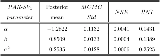
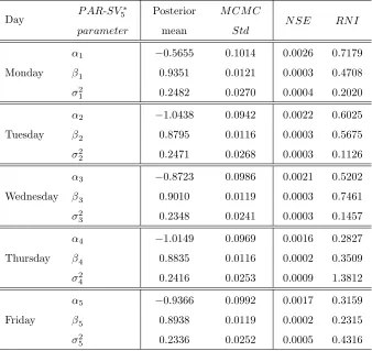
The Bayes Griddy-Gibbs parameter estimatebBGG of is taken to be the posterior mean =E( =")
which is, under the Markov chain ergodic theorem, approximated with any desired degree of accuracy by
bBGG= M1 MX+l0
l=l0
(l)
;
where (l)is thel-th draw of fromf( ; h=")given by Algorithm 3.1,l0 is the burn-in size, i.e. the number of initial draws discarded, andM is the number of draws.
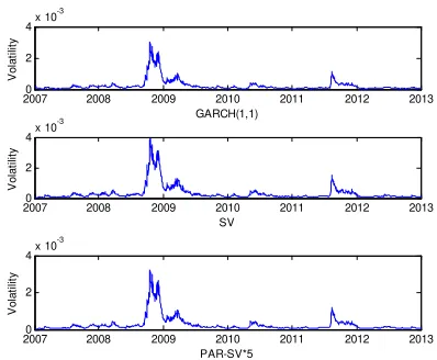
Smoothing and forecasting volatility are obtained as a by-product of the Bayes Griddy-Gibbs method.
The smoothed value, ht = E(ht="), of ht (1 t T) is obtained while sampling from the distribution
f(ht=")which in turn is the marginal of the posterior distributionf( ; h="). SoE(ht=")may be accurately
approximated by M1 PM+l0
l=l0 h
(l)
t where h
(l)
t is thel-th draw of ht fromf( ; ht="). Forecasting future values
hT+1; hT+2; ::; hT+k are obtained either as in the above using the log-volatility equation with the Bayes
parameter estimates, or directly while sampling from the predictive distribution f(hT+1; hT+2; ::; hT+k=")
(see also Jacquier etal, 1994).
3.2.4 M CM C diagnostics
It is important to discuss the numerical properties of the proposed BGGmethod in which the volatilities
are sampled element by element. Despite the ease of implementation, it is well documented that the main
drawback of the single-move approach (e.g. Kim et al, 1998) is that the posterior draws are often highly
correlated thereby resulting in a slow mixing and so a slow convergence properties. Among severalM CM C
diagnostic measures, we consider here the Relative Numerical Ine¢ciency (RN I) (e.g. Geweke,1989; Geyer,
1992), which is given by
RN I= 1 + 2
B X
k=1
K k
B bk;
where B = 500 is the bandwidth, K(:) is the Parzen kernel (e.g. Kim et al, 1998) and bk the sample
autocorrelation at lagkof theBGGparameter draws. TheRN I indicates in fact on the ine¢ciency due to
the serial correlation of theBGGdraws (see also Geweke,1989; Tsiakas,2006). AnotherM CM Cdiagnostic
measure (Geweke, 1989) we use here is the Numerical Standard Error (N SE), which is the square root of
the estimated asymptotic variance of theM CM C estimator. In fact, theN SE is given by
N SE=
v u u t1
M b0+ 2
B X
k=1
K Bk bk
!
;
wherebk is the sample autocovariance at lagkof theBGGparameter draws,K(:)is the Parzen kernel and
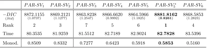
3.2.5 Period selection via the Deviance Information Criterion
An important issue inP AR-SVS modeling is the selection of the periodS. This problem is especially more
pronounced for modeling daily returns because their periodicity is not as obvious as in quarterly or monthly
data. Although many authors (e.g. Franses and Paap, 2000; Tsiakas, 2006) have emphasized the
day-of-the-week e¤ect in daily stock returns, which often entails a period ofS = 5, the period-selection problem in
periodic volatility models remains a challenging problem. Standard order-selection measures such as theAIC
andBIC, which require the speci…cation of the number of free parameters in each model, are not applicable
for comparing complex Bayesian hierarchical models like theP AR-SVS model. This is because in theP AR
-SVS model, the number of free parameters, which is augmented by the latent volatilities that are in fact not
independent but Markovian, is not well de…ned (cf. Berg etal,2004). For a long time, the Bayes factor has
been viewed as the best way to carry out Bayesian model comparison. However, its calculation based on
evaluating the marginal likelihood requires extremely high-dimensional integration, and this would be more
computationally demanding especially for P AR-SVS model which involves a larger number of parameters
augmented by the volatilities, exceeding the sample size.
In this paper, we will carry out period selection using rather theDeviance Information Criterion(DIC),
which may be viewed as a trade-o¤ between model adequacy and model complexity (Spiegelhalter et al,
2002). Such a criterion, which represents a Bayesian generalization of the AIC, is easily obtained from
M CM C draws, needing no extra-calculations. The (conditional)DIC as introduced by Spiegelhalter et al
(2002)is de…ned in the context ofP AR-SVS to be
DIC(S) = 4E ;h="(log (f("= ; h))) + 2 log f "= ; h ;
where f("= ; h) is the (conditional) likelihood of the P AR-SVS model for a given period S and ; h =
E(( ; h)=")is the posterior mean of( ; h). From the Griddy-Gibbs draws, the expectationE ;h="(log (f("= ; h)))
can be estimated by averaging the conditional log-likelihood,logf("= ; h), over the posterior draws of( ; h).
Further, the joint posterior mean estimate of( ; h)can be approximated by the mean of the posterior draws of
( (l); h(l)). Using the fact thatf("= ; h) :=f("=h) = 1 2
PT
t=1 log (2 ht) +
"2
t
ht , theDIC(S)is estimated
by
2
M l0X+M
l=l0
T X
t=1
log 2 h(tl) +
"2
t
h(tl)
! T X
t=1
log 2 ht +"
2
t
ht
;
where h(tl) denotes thel-thBGGdraw of ht fromf(ht="t; ), M is the number of draws, l0 is the burn-in size andht:=E(ht=")is estimated by M1 Pll0=+l0Mh
(l)
t (1 t n). Of course, a model is preferred if it has
the smallestDIC value.
Since the DIC is random and for the same …tted series it may change value from a M CM C draw to
al (2004), no e¢cient method has been developed for calculating reasonably accurate Monte Carlo standard
errors ofDIC. Nevertheless, following the recommendation of Zhu and Carlin(2000)we simply replicate the
calculation ofDIC someGtimes and estimateV ar(DIC)by its sample variance, giving a broad indication
of the implied variability ofDIC.
Note …nally that for the class of latent variable models to which belongs theP AR-SVS model, there are
in fact several alternative de…nitions of theDIC depending on the di¤erent concepts of the likelihood used
(complete, observed, conditional) and the one we worked with here is theconditional DIC as categorized
by Celeux etal (2006). We have avoided using theobserved DIC because, like the Bayes factor, it is based
on evaluating the marginal likelihood whose computation is typically very time-consuming.
4. Simulation study: Finite-sample performance of the
QM L
and
BGG
estimates
In this Section, a simulation study is undertaken to assess the performance of the QM L, BGG Bayes
estimates in …nite samples.
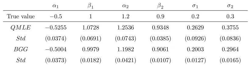
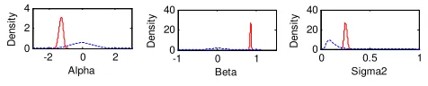
Concerning …nite-properties of theQM LandBGGestimates, three instances of the GaussianP AR-SVS
model with period S = 2 are considered and are reported respectively in Table 4.1, Table 4.2 and Table
4.3. The parameter = 1; 1; 2; 2; 21; 22 0
are chosen for each instance in order to be in accordance
with empirical evidence. In particular, for the three instances the persistence parameter 1 2 equals 0:90,
0:95and 0:99 respectively. We have also set small values for 2
1 and 22 because it is a critical case for the performance of theQM LE as pointed out by Ruiz(1994)and Harvey etal (1994)in the standardSV case.
The choice ofS = 2is motivated by computational and time-consuming considerations. For each instance,
we have considered 1000 replications of P AR-SVS series with sample size 1500, for which we calculated
the QM L and Bayes Monte Carlo replications. Mean of estimates (bQM L andbBGG) and their standard
deviations (Std) over the 1000 replications are reported in Tables 4.1-4.3.
For the QM L method a non linear optimization routine is required. We have applied a Gauss-Newton
type algorithm starting from di¤erent values of the parameter estimate. For the Bayes Griddy Gibbs
estimate, we have taken the same prior distributions for!= ( 1; 1; 2; 2) 0
across instances:
! N(!0; diag(0:05;0:5;0:05;0:5)),!0= (0;0;0;0)0;
1
2 1
2 5; 12
2
2 5;
Gibbs sampler is taken to be the volatility generated by the …ttedGARCH(1;1), that ish(0)=hG where 8
< :
"t=
p
hG
t t
hG
t ='0+'1"2t 1+ hGt 1
; t2Z;
while the initial log-volatility parameter estimate (0) is taken to be the ordinary least-squares estimate of
based on the serieslog h(0) . Furthermore, in the Griddy Gibbs iteration, htis generated using500grid
points and the range ofhtat thel-th Gibbs iteration is taken as in(3:12). Finally, the Gibbs sampler is run
for5500iterations from which we discarded the …rst500 iterations.
1 1 2 2 1 2
True value 0:5 1 1:2 0:9 0:2 0:3
QM LE
Std
0:5255
(0:0374)
1:0728
(0:0691)
1:2536
(0:0743)
0:9348
(0:0385)
0:2629
(0:0926)
0:3755
(0:0836)
BGG
Std
0:5004
(0:0373)
0:9979
(0:0182)
1:1982
(0:0421)
0:9061
(0:0107)
0:2003
(0:0127)
0:2964
[image:27.612.100.509.206.313.2](0:0165)
Table 4.1: Instance 1- Simulation results for QM LandBGGon a Gaussian P AR-SV2
withT = 1500:
1 1 2 2 1 2
True value 0:5 1 1:2 0:95 0:1 0:2
QM LE
Std
0:5258
0:0396
1:0799
0:0587
1:2527
0:0643
0:9849
0:0531
0:1394
0:5697
0:2570
0:4582
BGG
Std
0:4:939
0:0133
0:9992
0:0166
1:2030
0:0113
0:9505
0:0105
0:1004
0:0123
0:2069
[image:27.612.122.491.373.481.2]0:0093
Table 4.2: Instance 2- Simulation results for QM LandBGGon a Gaussian P AR-SV2