Tensor Centric Warfare I: Tensor Lanchester Equations

(1)

ISSN Online: 2153-0661 ISSN Print: 2153-0653

DOI: 10.4236/ica.2018.92002 May 30, 2018 11 Intelligent Control and Automation

Tensor-Centric Warfare I: Tensor Lanchester

Equations

Vladimir Ivancevic

1

, Peyam Pourbeik

2

, Darryn Reid

1

1_{Joint and Operations Analysis Division, Defence Science & Technology Group, Adelaide, Australia} 2_{Cyber and Electronic Warfare Division, Defence Science & Technology Group, Adelaide, Australia}

Abstract

We propose the basis for a rigorous approach to modeling combat, specifically under conditions of complexity and uncertainty. The proposed basis is a ten-sorial generalization of earlier Lanchester-type equations, inspired by the contemporary debate in defence and military circles around how to best util-ize information and communications systems in military operations, includ-ing the distributed C4ISR system (Command, Control, Communications, Computing, Intelligence, Surveillance and Reconnaissance). Despite attracting considerable interest and spawning several efforts to develop sound theoreti-cal frameworks for informing force design decision-making, the development of good frameworks for analytically modeling combat remains anything but decided. Using a simple combat scenario, we first develop a tensor generaliza-tion of the Lanchester square law, and then extend it to also include the Lan-chester linear law, which represents the effect of suppressive fire. We also add on-off control inputs, and discuss the results of a simple simulation of the fi-nal model using our small scenario.

Keywords

Tensor Modeling of Complex Warfighting, Lanchester-Type Combat Equations, C4ISR Military System

1. Introduction

Since at least the time of the Military Enlightenment, military organizations have invested considerable effort into developing theories of war and battle. The purpose of such theories is ultimately to inform decisions: what equipment to acquire, what processes to institute, what training and education to develop,

How to cite this paper: Ivancevic, V., Pourbeik, P. and Reid, D. (2018) Ten-sor-Centric Warfare I: Tensor Lanchester Equations. Intelligent Control and Auto-mation, 9, 11-29.

https://doi.org/10.4236/ica.2018.92002

Received: April 17, 2018 Accepted: May 27, 2018 Published: May 30, 2018

http://creativecommons.org/licenses/by/4.0/

(2)

DOI: 10.4236/ica.2018.92002 12 Intelligent Control and Automation

what research to conduct, how to conduct operations, and what operations to conduct in the first place. Perhaps unsurprisingly, many such efforts at the de-velopment of theories of war and battle have been oriented around the idea of achieving something like a complete and correct theory by which future out-comes might be predicted and thereby the means of determining the means to guarantee, or at least maximize the chances of, obtaining the outcome one de-sires. This has remained a dominant theme in military thinking ever since the foundational works of early theorists such as Jomini [1], through adoptions into military domains other than land battles in the late 19th century and early 20th Century with military educators such as Mahan [2], into the middle of the 20th Century with increasingly technologically-oriented theorists such as Fuller [3] [4] and Hart [5], and into modern and even more heavily technologically fo-cussed instantiations such as Network Centric Warfare (NCW) [6] and Ef-fects-Based Operations (EBO) [7]. Classical attempts at mathematically model-ing military conflict occurred within this overarchmodel-ing tradition of military thinking, and consequently they manifest the same basic goal of yielding ma-thematical theories that are numerically predictive with respect to battle out-comes.

Yet as predicted even from the outset by Clausewitz [8], a programme aimed at developing theories predictive of outcomes is ultimately not possible, be-cause—to use modern mathematical language—the conditions of war and bat-tle are simply not ergodic. That is, the inherent complex nonlinearity of such systems yield strong limitations on what can be predicted about their out-comes; conditions are not static and distributions are not nicely behaved, making it not possible to sample from the unrealized future by collecting data about the past. As a result of his stance, Clausewitz set himself apart from both his contemporary Jomini and from most other military theorists since by shy-ing away from fixed and prescriptive theories—while nonetheless concedshy-ing that such ideas are possible within sufficiently narrowly constrained problem domains. It is thus sometimes remarked that Clausewitz’ focus is strategic ra-ther than tactical. More deeply, this point of view gives a basis that more me-thodologically focused than theory focused: we are here primarily concerned with the means of solving problems that are effectively unique, messy, un-der-specified, socially complex, evolving and for which there is generally a scarcity of available data. In other words, decision-making in military matters has all the characteristics of what are often now described as “wicked prob-lems” [9].

(3)

prob-DOI: 10.4236/ica.2018.92002 13 Intelligent Control and Automation

lem, however, is that NCW presented a discredited though intuitively appealing explanation for exactly how this is to occur, with practical consequences that have proven problematic [10] [11]; its methodological framework held that knowledge is the outcome of collecting and consuming data and that the accu-racy of the knowledge is a function of the amount of information and ability to process it. The slightly later EBO notion similarly concludes that information collection, dissemination and processing are crucial, yet arguably overstates the strength and usefulness for prediction of supposed connections between out-comes and ostensible causes. Therefore, instead of the NCW, we are talking about distributed C4ISR system (Command, Control, Communications, Com-puting, Intelligence, Surveillance and Reconnaissance); for one of its examples, see [12].

These observations may be seen in terms of the limitations of classical sys-tems engineering achievements in dealing with wicked problems [9]; the reme-dy was a methodological shift to essentially the kind of problem-solving ap-proach espoused and exemplified by Clausewitz, but fleshed out later by Popper and subsequent authors [13] [14]. This line of reasoning inspires our approach. As with most approaches to modeling combat, there can little doubt that con-nectivity is important, that the availability and quality of information matters; our explanation for why this is so departs from earlier methods in this that the networks at the heart of our model permit ideas to be tested more rapidly and more thoroughly. Thus we have in mind the ideas of problem-solving, where the problem choices are primarily of the wicked variety; it is not information per se that matters, but rather the ability to obtain information that reveals un-acceptable error in proposed solutions and problem formulation. The goal of our modeling thus shifts from predicting outcomes of combat directly to ques-tions about system control. In this paper and its successor we present a basis for a novel mathematical approach to modeling war and battle under the condi-tions of complexity and uncertainty as a step towards overcoming the limita-tions that have been so challenging to most models of combat outcomes pro-posed in the past.

2. Background

2.1. Lanchester Equations

In defence operation research community it is well known that classical Lanchester-Osipov combat equations (also called Lanchester-style mass action models [15] [16] [17])1_{include two forces, Red/Attacker’s strength:}

( )

:

R R t= → and Blue/Defender’s strength: B B t =

( )

:→, with their respective initial sizes R0 and B0 and their corresponding combat-effectiveness

coefficients kR and kB. Lanchester equations are of the following two basic

1_{We remark that before Lanchester and Osipov, similar mass action models in naval applications}

(4)

types:2

1) Lanchester square law for direct-aimed fire:

( )

(

)

( )

(

00

)

, with 0 , 0 ,

R R

B B

R k B R R k

B k R B B k

= − = >

(2)

where overdot denotes time derivative, and kR and kB denote individual

combat-rate coefficients for the Red and Blue forces, respectively (e.g., tank versus tank, concentration of fire).

2) Lanchester linear law for area—unaimed fire:

( )

(

)

( )

(

00

)

, 0 , 0 ,

BR BR

RB RB

R k BR R R k

B k RB B B k

= − = >

(3)

where kBR and kRB denote mixed combat-rate coefficients for Red and Blue

forces (e.g., artillery barraging an area without precise knowledge of target locations).

Although similar Lanchester-type models had been extensively used in the past Century, today they are widely regarded as grossly oversimplified represen- tations of modern warfare, at best. This motivates our effort towards a modeling methodology of much higher complexity, including both continuous and discrete spatiotemporal dynamics, as proposed in the present paper3_.

2.2. Brief Review of Recent Military Thinking

For the last two decades, modern defence forces have generally been investing considerable effort in shifting the basis for decision-making for force development, employment and conduct of operations beyond individuation around platforms. Regarding ships, aircraft, armored vehicles and soldiers, for instance, as the base atomic units of military forces that are then packaged 2_{Frequently used generalization of the classical Lanchester-Osipov models of combat force dynamics}

[15] [16] [17]—including two forces, Red/Attacker’s strength: R R t = ( ):→ and Blue/Defen- der’s strength: B B t = ( ):→, with their respective initial sizes R0 and B0 and their corres-ponding combat-effectiveness coefficients kR and kB—is the LPB model, proposed in 1960s by Peterson [21] and in 1990s by Bracken [22], which reads:

( )

0

( )

0

(

)

, , with 0 , 0 , , 0 ,

q p p q

B R R B

R= −k R B B= −k R B R =R B =B k k > (1) where the exponents p and q (such that 1+ − =p q α) need to be empirically determined. The conserved quantity in the LPB model (1), 2 2 _const

R B

k R k B− = is obtained by eliminating time t, separating and integrating. The Lanchester aimed-fire (or, square law) model:

( ) 0 ( ) 0 ( )

, , with 0 , 0 , , 0

R B R B

R= −k B B= −k R R =R B =B k k >

corresponds to p=1,q=0 and thus to α =2; and the unaimed-fire (or, linear law) model:

( ) 0 ( ) 0 ( )

, , with 0 , 0 , , 0

BR RB BR RB

R= −k BR B= −k RB R =R B =B k k >

corresponds to p q= =1 and thus α =0 in the LPB model (1) (for more technical details see, e.g. [23] and the references therein).

3_{Since we will be using tensor indices (subscripts and superscripts) and Einstein’s summation}

(5)

hierarchically yields separate Command and Control (C2) channels for different military functions, which are then attached to acicular organizations that necessarily centralism planning and coordination to achieve desired effects. The emergence of modern communications and information technology was consequently broadly seen as offering the potential to dissolve such crystalline arrangements in favor of military forces able to fluidly self-organize in rapidly changing situations to both counter threats and take advantage of opportunities, by enabling collaboration directly between elements formerly widely separated by hierarchy.

Other advances including those the fields of telecommunications, robotics, artificial intelligence and autonomous systems have further opened apparent opportunities for collaborative planning, coordination and rapid response; at its core, modern defence thinking seeks to achieve highly distributed C2 arrangements enabled by communications and information systems in which information can be rapidly disseminated while also being protected from outside interdiction and interference. The extreme instantiation of this lies in the idea that by the provision of such a system, together with the training and procedures to utilize it, “information superiority”—the ability to acquire, transport and process more information than the opposition—will deliver superior ability to apply the effects of military force, and thus at least maximum chances of winning, if not virtually guaranteed complete battlefield domination. The ability for foreseeable battlefield communication systems to provide an infrastructure sufficient to realism the required connectivity, the flawed nature of at least this kind of extreme account has been made manifest by the fact that apparently overwhelming forces, enjoying the full benefits of the best technology has to offer, can and do continue to lose to ostensibly backwards and inferior forces.

(6)

systems [11].

Recent years have seen a growing knowledge about, and interest in, the burgeoning knowledge across the sciences about complexity and uncertainty, among defence and military thinkers. The general emerging view is that defence and military matters feature burgeoning complexity of technological, social, economic, cultural and political varieties. Whether war and battle is really becoming more complex than in the past is highly debatable; what is more certain is that analytical and conceptual frameworks used in its study to inform force design decisions struggle to adequately account for effects that Clausewitz pondered 180 years ago. The objective of the present paper is to take a step in this direction by generalizing and making rigorous the study of information networks using tensor dynamics on battlespace manifolds, and integrating it with Lanchester-type attrition models.

3. System Input

3.1. From the Air Campaign Scenario to the Combat Tensor

To be able to compare our system with McLemore et al. [24] we need to have the same/similar system input and after computations to compare the outputs. In our scaled-down (toy) model we interpret their Table. Scenario forces, as fol-lows. From a collaborative perspective, in their Air Campaign Scenario, the Red forces are given by a Bipartite graph: 15× Fighter aircraft and 15× Sensor air-craft, which in our 9 × 9-case becomes: 4 Fighter aircraft and 5 Sensor aircraft4

(see Figure 1). Also, their Blue forces are given by a Tripartite graph: 10× Figh-ter aircraft, 10× Sensor aircraft and 10× New aircraft, which in our 9 × 9-case becomes: 3 Fighter aircraft, 3 Sensor aircraft and 3 New aircraft (see Figure 2).

To make our Red and Blue aircraft configurations more realistic, the identity 9-matrices (with the local feedback-loops) have been added to the Red and Blue adjacency matrices as:

no self-loops

0 0 0 0 1 1 1 1 1 1 0 0 0 1 1 1 1 1

0 0 0 0 1 1 1 1 1 0 1 0 0 1 1 1 1 1

0 0 0 0 1 1 1 1 1 0 0 1 0 1 1 1 1 1

0 0 0 0 1 1 1 1 1 0 0 0 1 1 1 1 1 1

Red : 1 1 1 1 0 0 0 0 0 1 1 1 1 1 0 0 0 0

1 1 1 1 0 0 0 0 0 1 1 1 1 0 1 0 0 0

1 1 1 1 0 0 0 0 0 1 1 1 1 0 0 1 0 0

1 1 1 1 0 0 0 0 0 1 1 1 1 0 0 0 1 0

1 1 1 1 0 0 0 0 0 1

 

 

 _{ ⇒}

 

 

including local self-loops

,

1 1 1 0 0 0 0 1 a b

 

 

 _{ ≡}

 

 



(4)

4_{Since we have a simplified 9 × 9-case, we do not have the same number of Fighter and Sensor}

(7)

[image:7.595.299.451.72.293.2]

Figure 1. Bipartite graph for the Red force,

including 4 Fighter aircraft and 5 Sensor aircraft.

Figure 2. Tripartite graph for the Blue force, including 3

Fighter aircraft, 3 Sensor aircraft and 3 New aircraft.

no self-loops

0 0 0 1 1 1 1 1 1 1 0 0 1 1 1 1 1 1

0 0 0 1 1 1 1 1 1 0 1 0 1 1 1 1 1 1

0 0 0 1 1 1 1 1 1 0 0 1 1 1 1 1 1 1

1 1 1 0 0 0 1 1 1 1 1 1 1 0 0 1 1 1

Blue : 1 1 1 0 0 0 1 1 1 1 1 1 0 1 0 1 1 1

1 1 1 0 0 0 1 1 1 1 1 1 0 0 1 1 1 1

1 1 1 1 1 1 0 0 0 1 1 1 1 1 1 1 0 0

1 1 1 1 1 1 0 0 0 1 1 1 1 1 1 0 1 0

1 1 1 1 1 1 0 0 0

 

 

 _{ ⇒}

 

 

including local self-loops

.

1 1 1 1 1 1 0 0 1 a b

 

 

 _{ ≡}

 

 

A

[image:7.595.255.491.336.523.2]

(8)

The graphs for our Red and Blue forces, defined by adjacency matrices with local self loops, a

b

 and a b

A , respectively, are presented, using default graph

embeddings in Mathematica®_{, in}_{Figure 3}_and_{Figure 4}_.

3.2. The Combat Tensors for the Red and Blue Forces

[image:8.595.260.485.211.431.2]

As a “soft” introduction to dynamics of vector and tensor fields on battlespace manifolds, we define here the Combat-tensors, as the following matrix products (i.e., tensor contractions):

Figure 3. Bipartite graph with local feedback loops for the

Red force, including 4 Fighter aircraft and 5 Sensor aircraft.

Figure 4. Tripartite graph with local feedback loops for the

[image:8.595.263.484.479.678.2]

(9)

( )

Red : a , a b , , Blue: a , a a ,

b xt = b cT xt Nb xt =Ab b xt

  

of the combat adjacency matrices a b

 and a b

A with the total Power tensors

( )

,

a b

T xt and a

( )

,

b x t

 . Each component of the Power tensors (9 × 9 of them on the battle-manifold M9_{; see next section) is defined as a sum of the sigmoid}

spatiotemporal kink functions Tanh ,

( )

x t and ArcTan ,

( )

xt .

4. TCW Battlespace

A set of all active and controllable degrees-of-freedom (DOFs) of an arbitrary complex system comprises the configuration manifold for that system (see [25]

for more technical details). For example, an nD configuration manifold for a humanoid robot is the set of all its movable joint angles. Following this fundamental manifold prescription, any battlespace (see [26] and the references therein) in TCW can be formally defined as the battle-manifold. In case of a very large battle-manifold Mn_{, it can be approximated with} n_{, where n, the total}

number of DOFs, can be in millions (using computational framework outlined in the Appendix).

Complex warfighting dynamics on such battle-manifolds is naturally defined as an interplay of spatiotemporal vector and tensor fields flowing on them. For defining tensor expressions, we will use the abstract tensor notation with Einstein’s summation convention upon repeated indices; see [27]-[32].

On any battle-manifold Mn_{we can observe a dynamic interplay of various}

Actors, all defined by various vector and tensor fields, depending on their complexity.

Simpler Actors are formally defined as spatiotemporal vector-fields,

( )

,

a a

v =v x t , similar to velocities and forces from classical mechanics, or flow-velocities and vortices from fluid mechanics, or Hamiltonian vector-fields from generalized mechanics [28] [29], or Hopfield-Grossberg vector-fields from neurodynamics [33].

The main Actors on any battle-manifold Mn_{are the Red and Blue vector-fields,}

( )

,

a

R xt and _Ba

( )

_x,_t _{, respectively, which represent either the Red-Blue}

populations, or any other power measure of the Red-Blue forces. The main supporting Actor is the combat-tensor a

( )

,

b x t

 , defined earlier, which belongs to this category; a

b

 commutes with any other 2nd-order tensor field of the same covariance on the same battle-manifold Mn_(e.g.

( ) ( )

, , ,

a a

b b

T x t S x t )—they can be added together as linear machines:

a a a a

b = b ±Tb ±Sb±  

All these tensor fields are spatiotemporal dynamical objects governed by tensor equations, similar to the elastic stress-strain relation: stress elasticitycd strain

ab Eab cd

σ = ε _.

5. Tensor Combat Equations

5.1. Basic Tensor Combat Equations

(10)

by _x₌

(

_x1_{, ,} _x9

)

_{, although all the calculations would equally work for any}

manifold dimension (up to millions, using the computational framework outlined in the Appendix). We start the TCW modeling with the tensor Lanchester square law, which is the following vector/tensor generalization of Equation (2):

Red : ,

Blue : ,

a a b

b

a a b

b

R kA B

B

κ

C R

= =

(6)

where the Red and Blue forces are now defined as vector-fields, _Ra ₌_Ra

( )

_x,_t

and _Ba ₌_Ba

( )

_x,_t _{, and their effectiveness coefficients are denoted by k and}_κ.

The tensor fields a a

( )

,

b b

A =A x t and a a

( )

,

b b

C =C x t represent the sum of their combat-tensors ( a

b

 and a b

N ), their total power (or stress-energy) tensors

( a a

( )

,

b b

S =S xt and a a

( )

,

b = b x t

  ), and the Red and Blue swarming matrices,

( )

,

a a

b = b x t

  and a a

( )

,

b = b x t

  from McLemore et al. [24], provided the swarming matrices have dimension of dimM :

R-C2 R-Power R-McL

Red : a a a a,

b b b b

A =_ ± S ± _

B-C2 B-Power R-McL

Blue : a a a a .

b b b b

C =N ±  ± 

For example, on a 9D battle-manifold M9_{, the basic tensor Lanchester Equation}

(6) expand as:

1 1 1 1 2 1 3 1 4 1 5 1 6 1 7 1 8 1 9

1 2 3 4 5 6 7 8 9 ,

R =kA B kA B+ +kA B +kA B +kA B +kA B +kA B +kA B +kA B

2 2 1 2 2 2 3 2 4 2 5 2 6 2 7 2 8 2 9

1 2 3 4 5 6 7 8 9 ,

3 3 1 3 2 3 3 3 4 3 5 3 6 3 7 3 8 3 9

1 2 3 4 5 6 7 8 9 ,

4 4 1 4 2 4 3 4 4 4 5 4 6 4 7 4 8 4 9

1 2 3 4 5 6 7 8 9 ,

5 5 1 5 2 5 3 5 4 5 5 5 6 5 7 5 8 5 9

1 2 3 4 5 6 7 8 9 ,

6 6 1 6 2 6 3 6 4 6 5 6 6 6 7 6 8 6 9

1 2 3 4 5 6 7 8 9 ,

7 7 1 7 2 7 3 7 4 7 5 7 6 7 7 7 8 7 9

1 2 3 4 5 6 7 8 9 ,

8 8 1 8 2 8 3 8 4 8 5 8 6 8 7 8 8 8 9

1 2 3 4 5 6 7 8 9 ,

9 9 1 9 2 9 3 9 4 9 5 9 6 9 7 9 8 9 9

1 2 3 4 5 6 7 8 9 ,

1 1 1 1 2 1 3 1 4 1 5

1 2 3 4 5

1 6 1 7 1 8 1 9

6 7 8 9 ,

B C R C R C R C R C R

C R C R C R C R

κ

= + + + +

+ + + +

2 2 1 2 2 2 3 2 4 2 5

1 2 3 4 5

2 6 2 7 2 8 2 9

6 7 8 9 ,

B C R C R C R C R C R

C R C R C R C R

κ

= + + + +

+ + + +

3 3 1 3 2 3 3 3 4 3 5

1 2 3 4 5

3 6 3 7 3 8 3 9

6 7 8 9 ,

B C R C R C R C R C R

C R C R C R C R

κ

= + + + +

+ + + +

4 4 1 4 2 4 3 4 4 4 5

1 2 3 4 5

4 6 4 7 4 8 4 9

6 7 8 9 ,

B C R C R C R C R C R

C R C R C R C R

κ

= + + + +

+ + + +

(11)

5 5 1 5 2 5 3 5 4 5 5

1 2 3 4 5

5 6 5 7 5 8 5 9

6 7 8 9 ,

B C R C R C R C R C R

C R C R C R C R

κ

= + + + +

+ + + +

6 6 1 6 2 6 3 6 4 6 5

1 2 3 4 5

6 6 6 7 6 8 6 9

6 7 8 9 ,

B C R C R C R C R C R

C R C R C R C R

κ

= + + + +

+ + + +

7 7 1 7 2 7 3 7 4 7 5

1 2 3 4 5

7 6 7 7 7 8 7 9

6 7 8 9 ,

B C R C R C R C R C R

C R C R C R C R

κ

= + + + +

+ + + +

8 8 1 8 2 8 3 8 4 8 5

1 2 3 4 5

8 6 8 7 8 8 8 9

6 7 8 9 ,

B C R C R C R C R C R

C R C R C R C R

κ

= + + + +

+ + + +

9 9 1 9 2 9 3 9 4 9 5

1 2 3 4 5

9 6 9 7 9 8 9 9

6 7 8 9 .

B C R C R C R C R C R

C R C R C R C R

κ

= + + + +

+ + + +

Similar expansions (though larger) hold for battle-manifolds of any dimensions and can be derived using the fast tensor package xTensor [34] for Mathemati-ca®.

Assuming, for simplicity, the coordinate independence (x=const), both sets of expanded Lanchester equations represent sets of coupled nonlinear ODEs, which can be directly numerically solved, for any given Red and Blue initial conditions: Ra

( )

0 =R0a, Ba

( )

0 =B0a, using any adaptive Runge-Kutta ODE-

solver (e.g. Cash-Karp, Fehlberg and Dormand-Prince integrators), or their corresponding manifold/Lie-group integrators (e.g. Runge-Kutta Munthe-Kaas).

In the general case of explicit coordinate dependence (x x=

( )

t ), we would be actually dealing with the set of the first-order nonlinear PDEs, which would all require spatial discretization (e.g., using the Method of Lines, as implemented in Mathematica), after which the above mentioned ODE-solvers can be used again.

The same computational algorithms will apply, in both cases (ODEs and PDEs), also for the extended tensor Lanchester equations, formulated as follows.

5.2. Adding the Lanchester Linear Law

Next, to include the Lanchester linear law Equation (3) into Equation (6), while keeping their covariance (so that each term represents a vector-field), we need to extend them with quadratic terms of the Lanchester unaimed-fire equations (linear law) as:5

Red : ,

Blue : ,

a a b ab c d

b b cd

a a b ab c d

b b cd

R kA B k F B R

B

κ

C R

κ

G B R

= +

(7)

where the fourth-order tensors ab cd

F and ab cd

G represent more complex, strategic, 5_{The Basic Red and Blue tensor combat Equations (6)-(7) are valid for any linear/flat manifold M}9_.

In case of a strongly nonlinear/curved manifold M9_{, they would need the additional connection}

(12)

tactical and operational, Red and Blue capabilities, which can be defined either as the outer products of various matrices from [24], or composed as triple tensor sums:

Red Red Red

Blue Blue Blue

strat tact oper ,

strat tact oper .

ab ab ab ab

cd cd cd cd

ab ab ab ab

cd cd cd cd

F

G

= ± ±

(8)

The basic Red and Blue tensor combat Equation (7) are implemented in Mathe-matica as the initial value problem for the following temporal vector-fields:

where the 2nd-order Red and Blue combat-tensors Aa b, and Ca b, are defined

via sparse adjacency matrices (4) and (5) as:

[ ]

(

[

]

[

]

)

[ ]

{ } { }

,

Table 0.1 , Tanh 2 3 ArcTan 3 2 RandomReal , , , , ,

a b

A sR a a t t a n b n

 = _ _ − + −  

[ ]

(

[

]

[

]

)

[ ]

{ } { }

,

Table 0.1 , Tanh 3 4 ArcTan 2 5 RandomReal , , , , ,

a b

C sB a a t t a n b n

 = _ _ − + −

 

and the 4th-order (strategic + tactical + operational) tensors Fa b c d, , , and , , ,

a b c d

G are defined as:

[

]

[ ]

(

)

[ ]

{ } { } { } { }

, , ,

Table 0.01 0.1Sech 3 2 0.1Exp 3 0.01Sin 4 RandomReal , , , , , , , , ,

a b c d

F t t t

a n b n c n d n

 = − + − + −  

[

]

[ ]

(

)

[ ]

{ } { } { } { }

, , ,

Table 0.01 0.1Sech 2 3 0.1Exp 4 0.01Cos 3 RandomReal , , , , , , , , .

a b c d

G t t t

a n b n c n d n

 = − + − + −





A sample simulation of the basic tensor combat Equation (7) is performed in Mathematica (see Figures 5-7) for 10 time units (to match the simulations given in [24]) and random initial conditions.

5.3. Interpretation of Dynamical Simulations

(13)

[image:13.595.257.492.73.215.2]

Figure 5. Sample simulation of the basic tensor combat

[image:13.595.258.489.279.426.2]

Equation (7) for 10 time units with random initial conditions: monotonic dynamics of Red forces.

Figure 6. Sample simulation of the basic tensor combat

Equation (7) for 10 time units with random initial conditions: monotonic dynamics of Blue forces.

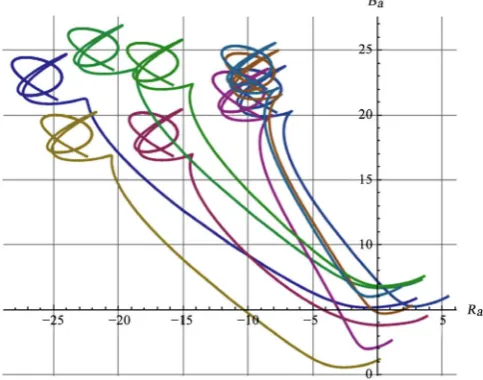
Figure 7. Sample simulation of the basic tensor combat Equation

[image:13.595.252.494.490.680.2]

(14)

[image:14.595.243.501.334.441.2]

In contrast, the output from [24] presented in their Chart 1 (Blue) and Chart 2 (Red) does not show the actual dynamics of the simulation, but rather the statis-tical inference from that simulation. Their main point is the “kill” of the aircraft, which they plotted along the same time axes (10 units) that we are using for the simulation. The 9 conflict points in our phase plane (Figure 7) are the points of potential “kill”; by relating to the Red and Blue time evolutions (in Figure 5 and

Figure 6) we can also infer who was “killed” or “degraded” at that same time point, as compared to their Chart 1 and Chart 2.

Based on this interpretation, we can see that our proposed tensor framework is capable of addressing the similar questions as those addressed by [24]. In the subsequent paper [25] we will extend this tensor Red-Blue dynamics to model warfare uncertainty.

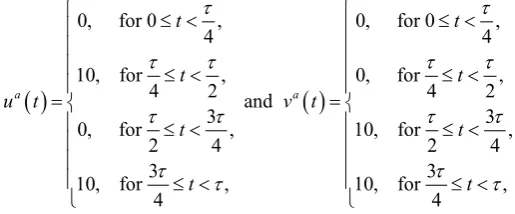
5.4. Adding Bang-Bang Control Actions

For the purpose of recasting the combat-dynamics Equations (7) into a control system, we will add to both Red and Blue forces simple-and-strong bang-bang (on-off) control inputs _{u t}a

( )

_and _{v t}a

( )

_{of the form:}

( )

0, for 0 , 0, for 0 ,

4 4

10, for , 0, for ,

4 2 _and 4 2

3 3

0, for , 10, for ,

2 4 2 4

3 3

10, for , 10, for ,

4 4

a a

t t

u t v t

t t

τ τ

τ τ τ τ

τ _τ τ _τ

 _{≤ <}  _{≤ <}

 

 _{≤ <}  _{≤ <}

 

=_ =_

 _{≤ <}  _{≤ <}

 

 _{≤ <}  _{≤ <}

 

where

τ

is the total simulation time (in our case τ=10 time units, to match the scenario from [24]).

In this way, we obtain the controlled tensor Red-Blue equations:

Red : ,

Blue : .

a a b ab c d a

b b cd

a a b ab c d a

b b cd

R kA B k F B R u

B

κ

C R

κ

G B R v

= + +

(9)

The basic vector control inputs _{u t}a

( )

_and _{v t}a

_{( )}

_{are implemented in}

Ma-thematica (in the scalar form) as:

[ ]

_ 10Piecewise 0,0 , 1, , 0, 3 , 1,3 ,

4 4 2 2 4 4

u t = __ ≤ <t τ_{ }  τ ≤ <t τ _{ } τ ≤ <t τ_{ }  τ ≤ <t τ__

       

 

 

[ ]

_ 10Piecewise 0,0 , 0, , 1, 3 , 1,3 ,

4 4 2 2 4 4

v t =  ≤ <t τ   τ ≤ <t τ   τ ≤ <t τ   τ ≤ <t τ

       

 

 

(15)

A sample simulation of the bang-bang controlled tensor combat Equation (9) is performed in Mathematica (see Figures 8-10) for 10 time units and random initial conditions.

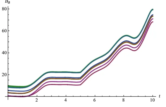
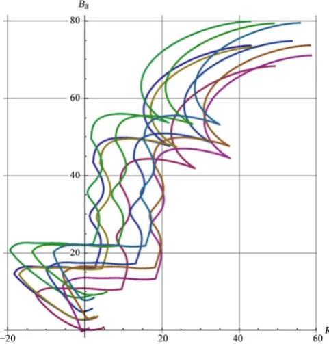
From Figures 8-10 we can see that adding strong bang-bang control inputs to tensor combat equations completely changes the natural combat-dynamics be-havior—control actions have the overall flattening effect. Even if the control in-puts have lower amplitudes (e.g., 5 instead of 10) the outcome would be qualita-tively similar: both the time-plots and the phase plot would be flattened out. From these computational observations we can infer that adding artificial con-trol inputs to natural Red-Blue combat dynamics does not make real sense, be-cause in reality the Red and Blue forces mutually control each other.

6. Conclusion and Future Work

[image:15.595.233.515.298.472.2]

We have presented the basic development of the tensor-centric warfare (TCW),

Figure 8. Sample simulation of the bang-bang controlled tensor Equation (9)

for 10 time units with random initial conditions: dynamics of Red forces.

Figure 9. Sample simulation of the bang-bang controlled tensor Equation (9)

[image:15.595.236.517.521.702.2]

(16)

[image:16.595.251.492.73.325.2]

Figure 10. Sample simulation of the bang-bang controlled tensor

Equation (9) for 10 time units with random initial conditions: Red-Blue phase plots.

as a tensor union and generalization of classical Lanchester combat equations and modern intention to orient the conduct of defence and military deci-sion-making around functions that cross traditional hierarchical lines of com-mand. Recognizing both the debates that continue about how best to do this and the limitations and weaknesses in military theories intended to inform and drive these developments, we have picked up the central feature of information and communications systems as a base infrastructure in future force design. The emphasis in our formalization lies in the possibility of better addressing the complexity and uncertainty inherent in war and battle, which, despite having been studied since the Military Enlightenment period, have continued to prove challenging to military thinking. In the sequel to this paper, presented in [25], we are extending this basic development with entropic modeling of warfare un-certainty and symmetry.

Acknowledgements

The authors are grateful to Dr. Tim McKay and Dr. Brandon Pincombe, Joint and Operations Analysis Division, Defence Science & Technology Group, Aus-tralia—for their constructive comments which have improved the quality of this paper.

References

(17)

[2] Mahan, A.T. (2003) The Influence of Sea Power upon History: 1660-1783. Pelican Pub. Co., Gretna. (Original Publication 1890)

[3] Fuller, J.F.C. (1926) The Foundations of the Science of War. Hutchinson and Com-pany, London. https://archive.org/details/foundationsofsci00jfcf

[4] Fuller, J.F.C. (1942) Machine Warfare: An Enquiry into the Influence of Mechanics on the Art of War. Hutchinson, London.

[5] Hart, B.H. (1967) Liddell: Strategy. 2nd Revised Edition, Fredrick A. Praeger Pub-lishers, New York.

[6] Alberts, D., Garstka, J. and Stein, F. (1999) Network Centric Warfare: Developing and Leveraging Information Superiority. CCRP.

[7] Davis, P.K. (2002) Effects-Based Operations: A Grand Challenge for the Analytical Community. RAND Corporation, Santa Monica, Arlington, and Pittsburgh. [8] von Clausewitz, C. (1989) In: Howard, M. and Paret, P., Eds., On War, Princeton

University Press.

[9] Rittel, H. and Webber, M. (1973) Dilemmas in a General Theory of Planning. Policy Sciences, 4, Elsevier, Amsterdam, 155-169. (Reprinted in Cross, N., Ed. (1984) De-velopments in Design Methodology, Wiley and Sons, Chirchester.)

[10] Reid, D.J., Goodman, G., Johnson, W. and Giffin, R.E. (2005) All That Glisters: Is Network-Centric Warfare Really Scientific? Defense and Security Analysis, 21, 335-367. https://doi.org/10.1080/1475179052000345403

[11] Reid, D.J. (2017) An Autonomy Interrogative. In: Abbass, H.A., Scholz, J. and Reid, D.J., Eds., Foundations of Trusted Autonomy, Springer, New York, 365-391. [12] Hui, P.P. (2011) OPAL—A Survivability-Oriented Approach to Management of

Tactical Military Networks. IEEE Military Communications Conference.

https://doi.org/10.1109/MILCOM.2011.6127450

[13] Popper, K. (2014) Conjectures and Refutations: The Growth of Scientific Know-ledge. Routledge, New York (First Published in 1963).

[14] Miller, D. (1998) Critical Rationalism: a Restatement and Defence. Open Court. [15] Lanchester, F.W. (1916) Aircraft in Warfare: The Dawn of the Fourth Arm.

Consta-ble, London.

[16] Lanchester, F.W. (2000) Mathematics in Warfare. In: Newman, J., Ed., The World of Mathematics, Vol. 4, Simon and Schuster, New York, 2138-2157.

[17] Osipov, M. (1995) The Influence of the Numerical Strength of Engaged Forces on Their Casualties. In: Helmbold, R.L. and Rehm, A.S., Trans., Warfare Modeling,

Military Operations Research Society, John Wiley & Sons, Hoboken, 290-343. [18] Chase, J.V. (1902) Sea Fights: A Mathematical Investigation of the Effect of

Supe-riority of Force in Combats upon the Sea. Naval War College Archives, RG 8, Box 109, XTAV.

[19] Fiske, B.A. (1905) American Naval Policy. U.S. Naval Institute Proceedings. [20] Baudry, A. (1912) La Bataille navale: Etudes sur les facteurs tactiques [The Naval

Battle: Studies of the Tactical Factors]. Translated by C. F. Atkinson, Hugh Rees, London.

[21] Peterson, R. (1967) On the Logarithmic Law of Combat and Its Application to Tank Combat. Operations Research, 15, 557-558. https://doi.org/10.1287/opre.15.3.557

[22] Bracken, J. (1995) Lanchester Models of the Ardennes Campaign. Naval Research Logistics, 42, 559-577.

(18)

[23] Keane, T. (2011) Combat Modelling with Partial Differential Equations. Applied Mathematical Modelling, 35, 2723-2735. https://doi.org/10.1016/j.apm.2010.11.057

[24] McLemore, C., Gaver, D. and Jacobs, P. (2016) A Model for Geographically Distri-buted Combat Interactions of Swarming Naval and Air Forces. Naval Research Lo-gistics, 63, 562-576. https://doi.org/10.1002/nav.21720

[25] Ivancevic, V., Reid, D. and Pourbeik, P. (to appear) Tensor-Centric Warfare II: En-tropic Uncertainty Modeling. ICA.

[26] Wikipedia (2017) Battlespace.

[27] Penrose, R. (2004) The Road to Reality. Jonathan Cape, London.

[28] Ivancevic, V. and Ivancevic, T. (2006) Geometrical Dynamics of Complex Systems. Springer, Dordrecht. https://doi.org/10.1007/1-4020-4545-X

[29] Ivancevic, V. and Ivancevic, T. (2007) Applied Differential Geometry: A Modern Introduction. World Scientific, Singapore. https://doi.org/10.1142/6420

[30] Ivancevic, V. and Ivancevic, T. (2008) Complex Nonlinearity: Chaos, Phase Transi-tions, Topology Change and Path Integrals. Springer, Berlin.

[31] Ivancevic, V. and Reid, D. (2015) Complexity and Control: Towards a Rigorous Behavioral Theory of Complex Dynamical Systems. World Scientific, Singapore. [32] Ivancevic, V., Reid, D. and Pilling, M. (2017) Mathematics of Autonomy:

Mathe-matical Methods for Cyber-Physical-Cognitive Systems. World Scientific, New Jer-sey/Singapore.

[33] Ivancevic, V. and Ivancevic, T. (2007) Neuro-Fuzzy Associative Machinery for Comprehensive Brain and Cognition Modelling. Springer, Berlin.

https://doi.org/10.1007/978-3-540-48396-0

[34] xTensor (2015) Fast Abstract Tensor Computer Algebra. http://xact.es/xTensor/ [35] EurekAlert! (12 June 2017) Blue Brain Team Discovers a Multi-Dimensional

Un-iverse in Brain Networks.

[36] Reimann, M., et al. (2017) Cliques of Neurons Bound into Cavities Provide a Miss-ing Link between Structure and Function. Frontiers in Computational Neuros-cience, 11, 48. https://doi.org/10.3389/fncom.2017.00048

[37] Bassett, D. and Sporns, O. (2017) Network Neuroscience. Nature Neuroscience, 20, 353-364. https://doi.org/10.1038/nn.4502

[38] Bauer, U., Kerber, M., Reininghaus, J. and Wagner, H. (2017) PHAT—Persistent Homology Algorithms Toolbox. Journal of Symbolic Computation, 78, 76-90.

https://doi.org/10.1016/j.jsc.2016.03.008

[39] (2017) AD: Automatic Differentiation. Hackage.

https://hackage.haskell.org/package/ad

[40] DiffSharp (2017) Differentiable Functional Programming.

(19)

Appendix: Computational Framework

A network-computational framework, with networks/tensors of up to millions of nodes, can be developed using the publicly available Matlab®_{toolbox supporting}

the cutting-edge topological research of brain cliques and cavities from compu-tational neuroscience (the Blue Brain project [35] [36] [37]). It is based on the persistent homology algorithms on directed simplices [38].

All tensor expressions can be derived using the tensor package xTensor [34]