warwick.ac.uk/lib-publications
Manuscript version: Author’s Accepted Manuscript
The version presented in WRAP is the author’s accepted manuscript and may differ from the published version or Version of Record.
Persistent WRAP URL:
http://wrap.warwick.ac.uk/109825
How to cite:
Please refer to published version for the most recent bibliographic citation information. If a published version is known of, the repository item page linked to above, will contain details on accessing it.
Copyright and reuse:
The Warwick Research Archive Portal (WRAP) makes this work by researchers of the University of Warwick available open access under the following conditions.
Copyright © and all moral rights to the version of the paper presented here belong to the individual author(s) and/or other copyright owners. To the extent reasonable and
practicable the material made available in WRAP has been checked for eligibility before being made available.
Copies of full items can be used for personal research or study, educational, or not-for-profit purposes without prior permission or charge. Provided that the authors, title and full
bibliographic details are credited, a hyperlink and/or URL is given for the original metadata page and the content is not changed in any way.
Publisher’s statement:
Please refer to the repository item page, publisher’s statement section, for further information.
Python Framework for HP Adaptive Discontinuous Galerkin
Method for Two Phase Flow in Porous Media
Andreas Dednera, Birane Kaneb, Robert Kl¨ofkornc, and Martin Nolted
aUniversity of Warwick, Coventry CV4 7AL UK
bUniversity of Stuttgart, Germany
cInternational Research Institute of Stavanger, Norway
dUniversity of Freiburg, Germany
April 15, 2018
Abstract
In this paper we present a framework for solving two phase flow problems in porous media. The discretization is based on a Discontinuous Galerkin method and includes local grid adaptivity and local choice of polynomial degree. The method is implemented using the new Python frontend Dune-FemPy to the open source framework Dune. The code used for the simulations is made available as Jupyter notebook and can be used through a Docker container. We present a number of time stepping approaches ranging from a classical IMPES method to fully coupled implicit scheme. The implementation of the discretization is very flexible allowing for test different formulations of the two phase flow model and adaptation strategies.
Keywords: DG, hp-adaptivity, Two-phase flow, IMPES, Fully implicit, Dune, Python,
Porous media
1
Introduction
Simulation of multi-phase flows and transport processes in porous media requires careful nu-merical treatment due to the strong heterogeneity of the underlying porous medium. The spatial discretization requires locally conservative methods in order to be able to follow small concentrations [4]. Discontinuous Galerkin (DG) methods, Finite Volume methods and Mixed Finite Element methods are examples of discretization techniques achieving local conservation at the element level [16]. Application of DG methods to incompressible two-phase flow started within the framework provided by a decoupled approach called Implicit Pressure Explicit Sat-uration (IMPES) where first a pressure equation is solved implicitly and then the satSat-uration is advanced by an explicit time stepping scheme. Upwinding, slope limiting techniques, and
sometimes H(div)-projection were required in order to remove unphysical oscillations and to
ensure convergence to a solution.
In the fully implicit and fully coupled approach, the mass balances are usually discretized in time by the implicit Euler method, resulting in a fully coupled system of nonlinear equations that has to be solved at each time step. The main advantage of a fully implicit scheme is
the possibility of using significantly larger time step sizes, which can be crucial in view of long-term scenarios like atomic waste disposal. Commonly, rather simple, yet robust space-discretization schemes, like cell-centered or vertex-centered finite volume schemes, are used [4, 6]. Fully implicit DG schemes have been proposed in [17] and [18], where the schemes are formulated in two space dimensions for incompressible fluid phases and numerical tests are performed without any kind of adaptivity.
Bastian introduced in [5] a fully coupled symmetric interior penalty DG scheme for in-compressible two-phase flow based on a wetting-phase potential and capillary potential for-mulation. Discontinuity in capillary-pressure functions is taken into account by incorporating the interface conditions into the penalty terms for the capillary potential. Heterogeneity in absolute or intrinsic permeability is treated by weighted averages. A higher-order diagonally implicit Runge-Kutta method in time is used and there is neither post processing of the veloc-ity nor slope limiting. Only piecewise linear and piecewise quadratic functions are employed and no adaptive method is considered.
A general abstract framework allowing for an a-posteriori estimator for porous-media two-phase flow problem was introduced by Vohralik et al. [31]. This paved the way for an h-adaptive strategy for homogeneous two-phase flow problems [11]. However, it has not been applied to DG methods so far.
Finally, Darmofal et al. introduced recently a space-time discontinuous Galerkin
h-adaptive framework for 2d reservoir flows. Implicit estimators are derived through the use of dual problems [7, 8] and a higher-order discretization is performed on anisotropic, unstruc-tured meshes. Unfortunately, application to 3d problems and hp-adaptive strategies haven’t been considered yet.
In this paper, we implement and evaluate numerically interior penalty DG methods for in-compressible, immiscible, two-phase flow. We consider strongly heterogeneous porous media, anisotropic permeability tensors and discontinuous capillary-pressure functions. We write the system in terms of a phase-pressure/phase-saturation formulation.
Adams-Moulton schemes of first or second order in time are combined with an Interior Penalty DG discretization in space. This implicit space time discretization leads to a fully coupled nonlinear system requiring to build a Jacobian matrix at each time step for the Newton-Raphson method.
This paper extends our previous work in [22, 23] and [24]. We consider here new hp-adaptive strategies and compare the fully implicit scheme with the iterative IMPES scheme and the implicit iterative scheme. The implicit iterative scheme is based on the iterative IMPES approach presented in [28] and treats the capillary pressure term implicitly to ensure stability. We also provide a more comprehensive model framework allowing to conveniently implement and compare various two-phase flow formulations.
The implementation is based on the open-source PDE software framework Dune-FemPy,
which is a Python frontend for Dune-Fem [13] based on the new Dune-Python module [15]
and which adds support for the Unified Form Language [3]. It allows for a compact, legible
presentation of the different discretizations under consideration. We combine Dune-FemPy
with Jupyter [27] and Docker [9] to ensure reproducibility of our numerical experiments. The
adaptive grid implementation is based on Dune-Alugrid [2] and parts of the stabilization
mechanisms used are provided byDune-Fem-DG[14].
2
Mathematical Model
This section introduces the mathematical formulation of a two-phase porous-media flow. In all that follows, we assume that the flow is immiscible and incompressible with no mass transfer between phases.
2.1 Two-phase flow formulation
Let Ω be a polygonal bounded domain in Rd, d ∈ {2,3}, with Lipschitz boundary ∂Ω and
let T ∈R+. The flow of the wetting phase (e.g. water) and the nonwetting phase (e.g. oil,
gas) is described by Darcy’s law and the continuity equation (e.g. balance of mass) for each
phase α ∈ {w, n}[21]. In all that follows, we denote with subscript w the wetting phase
and with subscript nthe nonwetting phase. The unknown variables are the phase pressures
pw, pn : Ω×(0, T)→ Rand the phase saturations sw, sn : Ω×(0, T)→ R. For each phase
α ∈ {w, n}, the Darcy velocityvα: Ω×(0, T)→Rd is given by
vα=−λαK(∇pα−ραg) in Ω×(0, T) (1)
where λα : Ω×(0, T) → R is the phase mobility, K : Ω→ Rd×d is the absolute or intrinsic
permeability tensor of the porous medium, ρα : Ω×(0, T) → R is the phase density, and
g ∈Rd is the constant gravitational vector.
Phase mobilities λα : Ω×(0, T)→Rare defined by
λα=
krα
µα
, α∈ {w, n}, (2)
whereµα is the constant phase viscosity andkrα: Ω×(0, T)→Ris the relative permeability
of phaseα. The relative permeabilities are functions that depend nonlinearly on the phase
saturation (i.e. krα =krα(sα)). Models for the relative permeability are the van-Genuchten
model [30] and the Brooks-Corey model [10]. For example, in the Brooks-Corey model,
krw(sn,e) = (1−sn,e)
2+3θ
θ , krn(sn,e) = (sn,e)2(1−(1−sn,e)
2+θ
θ ), (3)
where the effective saturation sα,e is
sα,e=
sα−sα,r
1−sw,r−sn,r
, ∀α∈ {w, n}. (4)
Here, sα,r, α ∈ {w, n}, are the phase residual saturations. The parameter θ ∈[0.2,3.0] is a
result of the inhomogeneity of the medium.
For each phase α∈ {w, n}, the balance of mass yields the saturation equation
φ∂(ραsα)
∂t +∇ ·(ραvα) =ραqα, (5)
where φ : Ω → R is the porosity, qα : Ω×(0, T) → R is a source or sink term (e.g. wells
located inside the domain in the case of a reservoir problem).
In addition to (1) and (5) the following closure relations must also be satisfied:
sw+sn= 1, (6)
where pc(sn) : Ω×(0, T) → R is the capillary pressure, a function of the phase saturation.
For the Brooks-Corey formulation,
pc(sn,e) =pd(1−sn,e)−1/θ. (8)
Here,pd≥0 is the constant entry pressure, needed to displace the fluid from the largest pore.
In summary, the immiscible, incompressible two-phase flow formulation is
vα =−λαK(∇pα−ραg), α∈ {w, n}, (9)
φ∂sα
∂t +∇ ·(vα) =qα, α∈ {w, n}, (10)
sw+sn= 1, (11)
pn−pw=pc, (12)
where we search for the phase pressurespα and the phase saturations sα,α∈ {w, n}.
2.2 Model A: Wetting-phase-pressure/nonwetting-phase-saturation formu-lation
Considering the phases are incompressible (i.e. the densitiesρα are constant), we get a total
fluid conservation equation by summing the two mass balance equations from (10),
φ∂(sn+sw)
∂t +∇ ·(vn+vw) =qn+qw.
Thanks to relation (11),
∇ ·(vn+vw) =qn+qw.
From relation (9) we have
−∇ ·(λnK(∇pn−ρng) +λwK(∇pw−ρwg)) =qn+qw.
The last closure relation (12) allows to write
−∇ ·(λnK(∇pc+∇pw−ρng) +λwK(∇pw−ρwg)) =qn+qw.
Finally,
−∇ ·
(λw+λn)K∇pw+λnK∇pc−(ρwλw+ρnλn)Kg
=qw+qn.
To complete our system, we consider as second equation the nonwetting phase conservation relation
φ∂sn
∂t +∇ ·vn=qn.
Using relation (9) and (12) yields
φ∂sn
∂t − ∇ ·
λnK(∇pw−ρng)
− ∇ ·
λnK∇pc
We get therefore a system of two equations with two unknownspw and sn,
−∇ ·
(λw+λn)K∇pw+λnK∇pc−(ρwλw+ρnλn)Kg
=qw+qn, (13)
φ∂sn
∂t − ∇ ·
λnK(∇pw−ρng)
− ∇ ·
λnK∇pc
=qn. (14)
Substituting ∇pc=p0c(sn)∇sn for∇pc as in [21, 20], the system (13)-(14) becomes
−∇ ·
(λw+λn)K∇pw+λnp0cK∇sn−(ρwλw+ρnλn)Kg
=qw+qn, (15)
φ∂sn
∂t − ∇ ·
λnK(∇pw−ρng)
− ∇ ·
λnp0cK∇sn
=qn. (16)
In order to have a complete system, we add appropriate boundary and initial conditions. Thus, we assume that the boundary of the system is divided into disjoint sets such that
∂Ω = ΓD∪ΓN. We denote byν the outward normal to∂Ω and set
pw(·,0) =p0w(·) , sn(·,0) =s0n(·) , in Ω,
pw=pw,D , sn=sD , on ΓD×(0, T),
vα·ν=Jα , Jt=
X
α∈{w,n}
Jα , on ΓN ×(0, T).
Here, Jα∈R,α∈ {w, n}, is the inflow,s0n, p0w, sD, and pw,D are real numbers. In order to
make pw uniquely determined, we require ΓD 6=∅.
2.3 General model framework
We provide here a unified model framework allowing for the representation of the models introduced in the previous sections,
−∇ ·
App(s)∇p+Aps(s)∇s+Gp(s)
=qp, (17)
Φ∂ts− ∇ ·
Asp(s)(∇p−Pg) +Ass(s)∇s+Gs(s)
=qs. (18)
The model is described once the physical parameter functions A,G, andPg are known. For
Model A (i.e. (15)-(16)), we have for example p=pw, s=sn and
App(s) = (λn(s) +λw(s))K, Aps(s) =λn(s)p0c(s)K,
Asp(s) =λn(s)K, Ass(s) =λn(s)p0c(s)K,
Gs(s) = 0, Gp(s) =−(ρwλw(s) +ρnλn(s))Kg,
Pg =ρng,
qp =qw+qn, qs=qn.
3
Discretization
3.1 Space Discretization
Let Th = {E} be a family of non-degenerate, quasi-uniform, possibly non-conforming
par-titions of Ω consisting of Nh elements (quadrilaterals or triangles in 2d, tetrahedrons or
hexahedrons in 3d) of maximum diameter h. Let Γh be the union of the open sets that
coincide with internal interfaces of elements of Th. Dirichlet and Neumann boundary
inter-faces are collected in the set ΓhD and ΓhN. Let e denote an interface in Γh shared by two
elements E− and E+ of Th; we associate with e a unit normal vector νe directed from E−
to E+. We also denote by|e| the measure of e. The discontinuous finite element space is
Dr(Th) = {v ∈ L2(Ω) : v|E ∈ PrE(E) ∀E ∈ Th}, with r = (rE)E∈Th, PrE(E) denotes QrE
(resp. PrE) the space of polynomial functions of degree at mostrE ≥1 on E (resp. the space
of polynomial functions of total degree rE ≥1 onE). We approximate the pressure and the
saturation by discontinuous polynomials of total degrees rp = (rp,E)E∈Th andrs= (rs,E)E∈Th
respectively.
For any function q ∈ Dr(Th), we define the jump operator J·Kand the average operator {·}
over the interfacee:
∀e∈Γh, JqK:=qE−νe−qE+νe, {q}:= 1 2qE−+
1 2qE+,
∀e∈∂Ω, JqK:=qE−ν, {q}:=qE−.
In order to treat the strong heterogeneity of the permeability tensor, we follow [19] and
introduce a weighted average operator{·}ω:
∀e∈Γh, {q}ω =ωE−qE−+ωE+qE+,
∀e∈∂Ω, {q}ω =qE−.
The weights are ωE− =
k+
k++k−, ωE+ =
k−
k++k− with k− = νeTKE−νe and k+ = νeTKE+νe.
Here,KE− andKE+ are the permeability tensors for the elementsE− and E+.
The derivation of the semi-discrete DG formulation is standard (see [5], [19], [25]). First, we multiply each equation of (17)-(18) by a test function and integrate over each element, then we apply Green formula to obtain the semi-discrete weak DG formulation. The bulk integrals are thus given by:
Bp((p, s), ϕ; ¯s) =
X
E∈Th
Z
E
App(¯s)∇p+Aps(¯s)∇s
· ∇ϕ+ X
E∈Th
Z
E
Gp(¯s)· ∇ϕ−
X
E∈Th
Z
E
qpϕ
Bs((p, s), ϕ; ¯s) =
X
E∈Th
Z
E
Asp(¯s)(∇p−Pq) +Ass(¯s)∇s
· ∇ϕ+ X
E∈Th
Z
E
Gs(¯s)· ∇ϕ−
X
E∈Th
Z
E
qsϕ
The consistency terms on the skeleton are
Cp((p, s), ϕ; ¯s) =
X
e∈Γh∪Γh D∪ΓhN
Z
e
App(¯s)∇p+Aps(¯s)∇s+Gp(¯s) ω·JϕK,
Cs((p, s), ϕ; ¯s) =
X
e∈Γh∪Γh D∪ΓhN
Z
e
Asp(¯s)(∇p−Pq) +Ass(¯s)∇s+Gs(¯s) ω·JϕK.
constant:
Sp(p, ϕ) =σ
X
e∈Γh∪Γh D
Z
e
γepJpK·JϕK,
Ss(s, ϕ) =σ
X
e∈Γh∪Γh D
Z
e
γesJsK·JϕK.
We follow the suggestions from [1] and chooseσ=r(r+ 1) wherer is the highest polynomial
degree of the discrete spaces. The penalty termsδp andδs depend on the largest eigenvalues
ofApp(0.5) and Ass(0.5), respectively. For Model A they are given by
γep= max(δ+p, δ−p) 2k
+k−
k++k− ×
|e|
min(|E+|,|E−|)
,
γes= max(δ+s, δ−s) 2k
+k−
k++k− ×
|e|
min(|E+|,|E−|)
,
where
δp = (ln(0.5) +lw(0.5)) and δs=ln(0.5)p0c(0.5).
The two bilinear forms thus are
Fp((p, s), ϕ; ¯s) =Bp((p, s), ϕ; ¯s)−Cp((p, s), ϕ; ¯s) +Sp(p, ϕ),
Fs((p, s), ϕ; ¯s) =Bs((p, s), ϕ; ¯s)−Cs((p, s), ϕ; ¯s) +Ss(p, ϕ).
3.2 Time stepping
Denoting with (pi, si) the approximation to the solution in the discrete function space at some
point in timeti we use a simple one step scheme to advance the solution (pi, si) at timeti to
(pi+1, si+1) at the next point in time ti+1=ti+τ based on
Fp((pi+1, si+1), ϕ; ¯s) = 0, (19)
Z
(si+1−si)ϕ+τ Fsα((pi+1, si+1), ϕ; ¯s) = 0, (20)
defining for a given constantα∈[0,1] the bilinear form
Fsα((p, s), ϕ; ¯s) = (1−α)Fs((pi, si), ϕ;si) +αFs((pi+1, si+1), ϕ; ¯s). (21)
The starting point of the iteration (p0, s0) are taken as anL2projection of the functions given
by the initial conditions into the discrete space. In our tests we have always used α= 1 since
we were more interested in investigating the influence of ¯s. We also used a fixed time stepτ
throughout the whole course of the simulation although varying time steps can be easily used as well.
Different choices for ¯s lead to different approaches for handling the nonlinearities in the
pressure. We tested five different approaches described in the following:
Linear For this approach we simply take ¯s=si leading to a forward Euler time stepping
Implicit Taking ¯s = si+1 leads to a backward Euler scheme. The resulting fully coupled system is solved iteratively using a Newton method.
Iterative This is similar to the previous approach, replacing the Newton method by an
outer fixed point iteration to solve the system: we define ¯sk=si+1,k with ¯s0 =si and in each
step of the iteration we therefore solve for k≥0:
Fp((pi+1,k+1, si+1,k+1), ϕ;si+1,k) = 0, (22)
Z
(si+1,k+1−si)ϕ+τ Fsα((pi+1,k+1, si+1,k+1), ϕ;si+1,k) = 0. (23)
IMPES-iterative This results in an iterative scheme using an IMPES approach. This is
similar to the previous approach except that in each step of the iteration we solve
Fp((pi+1,k+1, si+1,k), ϕ;si+1,k) = 0, (24)
Z
(si+1,k+1−si)ϕ+τ Fsα((pi+1,k+1, si+1,k+1), ϕ;si+1,k) = 0. (25)
IMPES Finally we use a classical IMPES approach, which is similar to the previous without
carrying out the iteration: the saturation in the pressure equation is taken explicitly and the new pressure is used in the saturation equation (in contrast to the first approach where the old pressure is used).
Fp((pi+1, si), ϕ;si) = 0, (26)
Z
(si+1−si)ϕ+τ Fsα((pi+1, si+1), ϕ;si) = 0. (27)
With the exception of the first and the last approach, all methods use an iteration to obtain a fixed point to the fully implicit equation
Fp((pi+1, si+1), ϕ;si+1) = 0, (28)
Z
(si+1−si)ϕ+τ Fsα((pi+1, si+1), ϕ;si+1) = 0. (29)
In the third and the fourth method this is achieved using an outer iteration (based on the first or the last method, respectively) while the second method uses a Newton method. To make the approaches easier to compare, we use the same stopping criteria for the iteration in
all three cases. We take (pi+1, si+1) = (pi+1,l, si+1,l) withlsuch that
ksi+1,l−si+1,l−1kL2(Ω) <toliterksl−1kL2(Ω) . (30)
We use a value of toliter= 3·10−2 to stop the iteration when the relative change between two
steps is less then three percent.
3.3 Adaptivity
Different adaptive strategies are possible depending on how elements are refined/coarsened; whether the elements should be p-refined or h-refined; when should the refinement process be stopped (e.g. maximum level of refinement, stopping criterion). Keeping this in focus, we provide in this section a brief introduction to different adaptive strategies implemented
and tested in this work. In all that follows, the parameters maxpoldeg and maxlevel refer
3.3.1 Error indicator
In the sequel, we implement an explicit estimator originally designed for non-steady convection-diffusion problems. A thorough analysis is available in [29].
Applying the estimator to the phase conservation equation (18) yields:
η2E =h2EkRvolk2L2(E)+
1 2
X
e∈Γh
he
Re2
2
L2(e)+
1
he
Re1
2
L2(e)
+ X
e∈∂E∩∂Ω
he
Re2
2
L2(e)+
1
he
Re1
2
L2(e)
. (31)
HereRvol is the interior residual indicating how accurate the discretized solution satisfies the
original PDE at every interior point of the domain,
Rvol=qs−φ
∂s ∂t +∇ ·
Asp(s)(∇p−Pg) +Ass(s)∇s+Gs(s)
.
The termRe1 is the numerical zero order inter-element (resp. Dirichlet boundary condition)
residual depending on the jump of the discrete solution at the elements boundaries (resp. at the Dirichlet boundary), hence reflecting the regularity of the DG approximation (resp. the accuracy of the approximation on the Dirichlet boundary),
Re1 = (
σγesJsK ife∈Γ
h,
σγes(sD−s) ife∈ΓD.
The term Re2 is the first order numerical inter-element residual (resp. Neumann boundary
condition residual) depending on the jump of numerical approximation of the normal flux at the elements boundaries (resp. at the Neumann boundary). It also allows to assess the regularity of the DG approximation (resp. the accuracy of the approximation on the Neumann boundary),
Re2 = (
JAsp(s)(∇p−Pg) +Ass(s)∇s+Gs(s)K·νe ife∈Γ
h,
Jn+ Asp(s)(∇p−Pg) +Ass(s)∇s+Gs(s)
·νe ife∈ΓN.
3.3.2 Adaptive strategies
The indicator presented above will be used to drive adaptive algorithms. The h-adaptive
algorithm is depicted in Algorithm 1. Given the error indicator ηEr,n defined in equation (31)
for a polynomial degree r in time step n for each element E, we refine each element whose
error indicator is greater than a refinement threshold value hT olnE and we coarsen elements
where the indicator is smaller than the coarsening threshold 0.01×hT olnE.
In order to automatically compute the tolerance for refinementhT olEn used in each timestep
time steps and grid elements. As a result we computehT olEn based on the initially computed error indicator,
hT olnE :=tT ol τ
n
|Tn h |
with tT ol:= 1
T
X
E∈Th
ηEr,0. (32)
In the following we use ηEr = ηr,nE as abbreviation for ease of reading. The choice between
increasing or decreasing the local polynomial order depends heavily on the value of an
in-dicator ςE(ηrE, η
r−1
E ) where η
r
E, E ∈ Th is a given error indicator and ηEr−1 is the same
indi-cator evaluated for the L2 projection of the solution into a lower order polynomial space.
The derivation of this L2 projection is quite straightforward due to the hierarchical
as-pect of the modal DG bases implemented. We considered a marking strategy based on
the difference of ςE = |ηEr −ηrE−1|. When this difference on a given element is non zero
we expect the higher order to contribute to the accuracy of the scheme and keep or in-crease the given polynomial on that element otherwise the polynomial order is dein-creased.
Algorithm 1 h-adapt
1: LetηEr,nbe given
2: for allE∈ Thdo
3: hE=diam(E)
4: if ηr,nE >hT oln
EANDmaxlevel>level(E)then
5: hnew
E :=
hE
2
6: else ifηr,nE <0.01×hT oln
EANDlevel(E)>0then
7: hnewE := 2hE
8: else
9: hnew
E :=hE
10: end if
11: end for
Algorithm 2 p-adapt: markpDiff
1: LetςE be given
2: for allE∈ Thdo
3: rE:=poldeg(E)
4: ifςE<ptol then
5: ifrE>1 then
6: rnew
E :=rE−1
7: else
8: rnew
E :=rE
9: end if
10: else if ςE>100×ptol then
11: ifrE<maxpoldeg then
12: rnew
E :=rE+ 1
13: else
14: rnew
E :=rE
15: end if
16: else
17: rnew
E :=rE
18: end if
19: end for
3.4 Stabilization
Although due to the presence of the capillary pressure terms strong shocks do not occur in the numerical experiments carried out in this paper, the DG schemes needs stabilization to avoid unphysical values, such as negative saturation which would lead to an undefined state in equation (8).
We follow the approach from [12] which has been initially proposed by Zhang and Shu in [32]. The general idea is to scale each polynomial on each element such that a constraint on minimum and maximum values of the saturation is respected. We define the following
projection operator Πs:Dr(Th)−→ Dr(Th) with
Z
Ω
Πs[s]·ϕ=
Z
Ω
˜
s·ϕ ∀ϕ∈ Dr (33)
where on each element E of the grid we define a scaled saturation ˜s(x) :=χE s(x)−¯s
with ¯sbeing the mean value of son elementE. The scaling factor is
χE := min
x∈ΛE
{1,|(¯s−smin)/(¯s−s(x))|,|(smax−s¯)/(¯s−s(x))|} (34)
for the combined set of all quadrature points ΛE used for evaluation of the bilinear forms
defined earlier, i.e. interior and surface integrals.
The scaling limiter is applied after each Newton iteration for the implicit scheme and after each iteration of the iterative schemes.
4
Numerical Experiments
This section provides different numerical experiments aiming to demonstrate the effectiveness and robustness of the DG discretization of porous media flow models. All test are imple-mented with the hp-adaptive DG method described in the previous section using the different approaches for the time step computation. The maximal grid level was fixed to three and the maximal polynomial was also three. The main components of the code areddescribed in some detail in B and provide as part of a docker container as explained in A. We also show results based on some alternative approaches for example for the underlying model or for the adaptive strategy. These modifications to the python code are also provided in Appendix B. They demonstrate the flexibility of the Python code.
4.1 Problem setting
A container is filled with two kinds of sand and saturated by water with density ρw =
1000 Kg/m3 and viscosity µw = 1×10⁻³ Kg/m s. The dense non-aqueous phase liquid
(DNAPL) considered in the experiment is Tetrachloroethylene with densityρn= 1460Kg/m3
and viscosity µn= 9×10⁻⁴ Kg/m s.
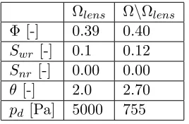
We consider a two-dimensional DNAPL infiltration problem with different sand types and anisotropic permeability tensors. The material properties are detailed in Table 1. The bottom
of the reservoir is impermeable for both phases. Hydrostatic conditions for the pressure pw
and homogeneous Dirichlet conditions for the saturation sn are prescribed at the left and
right boundaries. A flux of Jn=−5.137×10⁻⁵ m s−1 of the DNAPL is infiltrated into the
domain from the top. Detailed boundary conditions are specified in Figure 1 and Table 2. Initial conditions where the domain is fully saturated with water and hydrostatic pressure
distribution are considered (i.e. p0w = (0.65−y)·9810, s0n = 0). The permeability tensor
KΩ\Ωlens of the domain Ω\Ωlens is
KΩ\Ωlens =
10−10 −5×10⁻¹¹
−5×10⁻¹¹ 10−10
!
m2
and the permeability tensorKΩlens of the lens Ωlens is
KΩlens =
6×10⁻¹⁴ 0
0 6×10⁻¹⁴
!
m2.
The coarsest (macro) mesh consists of 60 quadrilateral elements globally refined everywhere
we later plot the solution ofsover the line
x(σ) = (1−σ)(0.25,0.65)T +σ(0.775,0.39)T (35)
with σ ∈[0,1]. Snapshots of the evolution of the resulting flow and the grid structure are
DNAPL
0
.
26
m
0
.
06
m
0.9m
Ω
Ωlens
0.39m 0.51m
0.34m 0.56m
DNAPL
ΓE ΓW
ΓS
Ω
Ωlens
ΓN
ΓN ΓIN
[image:13.612.90.518.183.263.2]x(σ) .
Figure 1: Geometry and boundary conditions for the DNAPL infiltration problem. The purple line
in the right picture is described byx(σ) from equation (35).
Ωlens Ω\Ωlens
Φ [-] 0.39 0.40
Swr [-] 0.1 0.12
Snr [-] 0.00 0.00
θ [-] 2.0 2.70
[image:13.612.84.218.321.409.2]pd [Pa] 5000 755
Table 1: 2d problem parameters.
ΓIN Jn=−5.137×10⁻⁵,Jw = 0
ΓN Jn= 0.00, Jw= 0.00
ΓS Jw = 0,Jn= 0.00
ΓE∪ΓW pw = (0.65−y)·9810,sn= 0
Table 2: 2d problem boundary conditions.
shown in Figure 2.
4.2 Time step stability
In this section we compare the various splitting and solution strategy described in Section 3.2. We compare three implicit and iterative coupling schemes and two loosely coupled schemes, one of them the classical IMPES scheme.
Forτ >3 only the fully coupled schemes are able to produces reasonable solutions. This is illustrated in Figure 3.
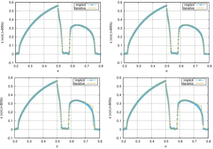
In Figure 4 we compare the solution of the various fully coupled schemes for different time step sizes. If the solution converges then a correct solution profile is produced. The stability
Figure 2: Evolution of the non wetting saturationsn at times t= 200,400,600, and t= 800
[image:13.612.300.505.331.391.2] [image:13.612.82.519.600.705.2]-0.1 0 0.1 0.2 0.3 0.4 0.5 0.6
0.2 0.3 0.4 0.5 0.6 0.7 0.8
s (x( σ ),t=800s) σ implicit iterative impesIterative impes linear -0.1 0 0.1 0.2 0.3 0.4 0.5 0.6
0.2 0.3 0.4 0.5 0.6 0.7 0.8
[image:14.612.91.505.111.254.2]s (x( σ ),t=800s) σ implicit iterative impesIterative impes linear
Figure 3: All schemes for τ = 3 (left) and τ = 5 (right). All schemes are able to capture
the solution characteristics for times steps smaller and up to τ = 3. Forτ >3 only the fully
coupled schemes are able to produce reasonable solutions, while the loosely coupled schemes do no longer capture the front position correctly.
of the implicit scheme is influenced by the fact that the stabilization operator is only applied before and after the Newton solver.
In principle the explicit coupling schemes work fine for small time steps and fail to produce a valid solution for larger time steps. Here, the implicit schemes show their strength allowing for faster computation once the time step is chosen sufficiently large.
-0.1 0 0.1 0.2 0.3 0.4 0.5 0.6
0.2 0.3 0.4 0.5 0.6 0.7 0.8
s (x( σ ),t=800s) σ τ=3 τ=5 τ=7 -0.1 0 0.1 0.2 0.3 0.4 0.5 0.6
0.2 0.3 0.4 0.5 0.6 0.7 0.8
s (x( σ ),t=800s) σ τ=3 τ=5 τ=7 τ=7 τ=9 τ=13
Figure 4: Left, the solution for fully coupled implicit scheme forτ = 3,5,7. Right the solution
for the IMPES-iterative scheme for τ = 3,5,7,9,11,13.
4.3 Cut off stabilization
In this section we study a very simple stabilization approach aining at finding a replacement for the more complicated scaling limiter described in Section 3.4. The idea is to simply replace
values for the saturation sbelow a given threshold smin and smax. Values of the saturation
outside of the region considered physical will cause problems when computing the capillary pressure. So in this approach we use a very simple cut off for guaranteeing that no non negative
values are used in the power laws required for the capillary pressure by replacing sw,e, sn,e by
[image:14.612.92.504.422.562.2]This approach can be directly incorporated into the symbolic description of the model as shown in C.1.
As can be clearly seen in Figure 4.3 significant over and undershoots are produced by all methods at the fronts. Both IMPES type splitting schemes fail to converge even for smaller time steps and the fully coupled implicit scheme produces wrong flow speeds even for
moderate values of τ. Only the iterative scheme manages to produce at least a reasonable
representation of the flow.
-0.1 0 0.1 0.2 0.3 0.4 0.5 0.6
0.2 0.3 0.4 0.5 0.6 0.7 0.8
s (x( σ ),t=800s) σ implicit iterative linear -0.1 0 0.1 0.2 0.3 0.4 0.5 0.6
0.2 0.3 0.4 0.5 0.6 0.7 0.8
s (x( σ ),t=800s) σ implicit iterative linear -0.1 0 0.1 0.2 0.3 0.4 0.5 0.6
0.2 0.3 0.4 0.5 0.6 0.7 0.8
[image:15.612.81.513.218.311.2]s (x( σ ),t=800s) σ implicit iterative linear
Figure 5: Left results forτ = 1, middleτ = 3 and rightτ = 5. The IMPES and impesIterative
scheme fail to converge with this approach. The other schemes all produce oscillations around the front. Interestingly, the fully coupled implicit also fails to compute the correct front position for increasing times steps.
4.4 Different model: Model B
In this section we compare our original model formulation with a description where the
two-phase flow problem is modeled as a system of equations with two unknowns ¯p and sn. Here
¯
p=pw+12pc:
−∇ ·
(λw+λn)K∇p¯+(λn
−λw)
2 p
0
cK∇sn−(ρwλw+ρnλn)Kg
=qw+qn on Ω×(0, T),
(36)
φ∂sn
∂t − ∇ ·
λnK(∇p¯−ρng)
−1
2∇ ·
λnp0cK∇sn
=qn on Ω×(0, T).
(37)
To complete the system, we add appropriate boundary and initial conditions.
¯
p(·,0) =p0w(·) +1
2pc(s
0
n(·)), sn(·,0) =s0n(·) , in Ω,
¯
p=pw,D+ 1
2pc(sD) , sn=sD , on Γ
D×(0, T),
vα·ν =Jα , Jt=
X
α∈{w,n}
Jα , on ΓN ×(0, T).
Here,Jα∈R,α∈ {w, n} is the inflow, s0n, p0w, sD, and pw,D are real numbers.
and
App(s) = (λn(s) +λw(s))K, Aps(s) =
λn(s)−λw(s)
2 p
0
c(s)K,
Asp(s) =λn(s)K, Ass(s) =
λn(s)
2 p
0
c(s)K,
Gs(s) = 0, Gp(s) =−(ρwλw(s) +ρnλn(s))Kg,
Pg =ρng,
qp =qw+qn, qs=qn.
The required changes to the Python code are again minimal and described in the C.2. In the following we investigate the stability of the different methods with respect to the
time step size when applied tomodelB. We perform the same investigation described in the
previous section where we used modelA. The results are summarized in Figure 6. We only
investigated the stability of the three methods implicit,iterative, and impes-iterative. For
modelB the splitting introduced in theimpes type approach failed even for τ = 1 while the
other two methods produce results in line with the results produced with modelA although
for higher values ofτ the iterative methods produce a discontenuety at the right most front
as can be seen in the plots on the bottom row of Figure 6. For τ > 5 the implicit method
fails, making modelB a less stable choice for this scheme. On the other hand the iterative
approach produced results also for larger time stepsτ = 9,11,13,15 (not shown here) but in
each case the solution showed the same type of discontinuety.
Taking all the approaches into account, it is clear that modelA is the more stable
rep-resentation of the problem. But our results also indicate that the stability of the iterative
scheme does not seem to depend so much on the choice of the model (at the least for the two versions tested) and produces very similar results in both cases.
4.5 P-adaptivity
Here we compare different approaches for the indicator used to set the local polynomial degree.
In the following we always use theimplicit method withτ = 5, h-adaptivity with a maximum
level of three and also a maximum level of three for the polynomial order. In addition to the approach used previously we test a version without p-adaptivity and an indicator based on determining the smoothness of the solution. In regions where the indicator detects a reduction in smoothness the polynomial order is reduced but only if the grid has been refined to the
maximum allowed level. The smoothness indicator is based onςE = η
r E
-0.1 0 0.1 0.2 0.3 0.4 0.5 0.6
0.2 0.3 0.4 0.5 0.6 0.7 0.8
s (x( σ ),t=800s) σ implicit iterative -0.1 0 0.1 0.2 0.3 0.4 0.5 0.6
0.2 0.3 0.4 0.5 0.6 0.7 0.8
s (x( σ ),t=800s) σ implicit iterative -0.1 0 0.1 0.2 0.3 0.4 0.5 0.6
0.2 0.3 0.4 0.5 0.6 0.7 0.8
s (x( σ ),t=800s) σ implicit iterative -0.1 0 0.1 0.2 0.3 0.4 0.5 0.6
0.2 0.3 0.4 0.5 0.6 0.7 0.8
[image:17.612.91.509.112.404.2]s (x( σ ),t=800s) σ implicit iterative
Figure 6: Results usingmodelB. Top row: τ = 1,3, bottom row: τ = 5,7.
Algorithm 3 p-adapt: markpFrac
1: LetςEbe given
2: for allE∈ Thdo
3: rE:=poldeg(E)
4: if ςE<0.01×ptol then
5: if rE<maxpoldeg then
6: rnew
E :=rE+ 1
7: else
8: rnew
E :=rE
9: end if
10: else if ςE>ptol then
11: if rE>1 then
12: rnew
E :=rE−1
13: else
14: rnew
E :=rE
15: end if
16: else
17: rnew
E :=rE
18: end if
19: end for
The changes to the code are described in C.3.
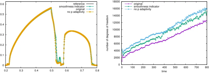
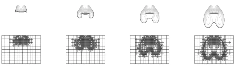
Figure 7 shows the distribution of the polynomial order for the two p-adaptive approaches. The local grid adaptivity is of course also influenced by the choice of indicator for the poly-nomial degree because the values of the residuals change. This can also be seen in Figure 7. As expected for the approach discussed in Section 3.3 the polynomial order is reduced to
[image:17.612.88.523.452.649.2]Figure 7: Comparison of different approaches for choosing the local polynomial degree. The top row shows the distribution of the polynomial order (left: original approach, right: modified
indicator). Red color refers to r= 3 and blue refers to r= 1. The bottom row shows the grid
level used for the three simulation. Red refers to l= 3 and blue refers tol= 0. Left to right:
original approach, modified indicator, with uniform polynomial degree of three. White lines
show 20 contour levels between sn= 0 and sn= 0.55.
0 0.1 0.2 0.3 0.4 0.5 0.6
0.2 0.3 0.4 0.5 0.6 0.7 0.8
reference smoothness indicator original no p adaptivity
0 2000 4000 6000 8000 10000 12000 14000 16000 18000
0 100 200 300 400 500 600 700 800
number of degrees of freedom
time original
smoothness indicator no p adaptivity
Figure 8: Comparison of different approaches for choosing the local polynomial degree. Shown
sn over the line in equation (35).
[image:18.612.98.503.352.497.2]Figure 9: Evolution of the non wetting saturation sn for the isotropic weak lens setting at
times t= 800,1600,2400, and t= 3200 (top) and the corresponding adaptive grid structure
(bottom).
simulation and still to 75% at the final time. The smoothness indicator given in this section only leads to a reduction of 20% at the beginning of the simulation and by only 6% at the final time.
Overall the indicator described in Section 3.3 does seem to lead to a better distribution of the polynomial degree with negligible influence of the actual solution. As can be seen from Figure 7, there is only little reduction of the order in the actual plume and the intermediate
order p = 2 is hardly used anywhere in the domain. Both these observations indicate that
further research into p-adaptivity for this type of problem is required.
4.6 Isotropic Flow over a weak Lens
In the final section we just study a second test case. The setup is the same as in the previous example but the permeability tensors is isotropic and the lens is weaker:
KΩ\Ωlens =
10−10 0
0 10−10
!
m2 , KΩlens =
10−12 0
0 10−12
!
m2 .
On the Python side the problem class the definition of K has to be modified accordingly as
shown in C.4.
Snapshots of the evolution of the resulting flow are shown in Figure 9. The symmetry is clearly visible both in the solution and in the grid refinement. The grid is locally refined at the interface and around the lens once the flow reaches that point. Dune to the weaker lens flow also passes through the lens. Overall our tests indicate that the conclusions obtained from our previous tests also apply to this setting.
5
Conclusion
We have presented a framework that allows to study hp-adaptive schemes for two-phase flow in porous media. The presented approach allows to easily study different adaptive strategies and time stepping algorithms. The change from one algorithm to another is easily implemented. All python based implementation is in the end forwarded to C++ based implementations to ensure performance of the applications.
Furthermore, the prototypes build on very mature implementations from the Dune
We focused in this paper mostly on the stability of different approaches for evolving the solution from one time step to the next. Our results indicate that IMPES type splitting schemes can be used when smaller time step are acceptable while for larger time steps schemes solving the fully coupled equations should be used. The simple fixed point iteration seems to work quite well and seems quite stable with respect to the algorithmic approaches and models tested. It turns out that the method does show convergence issues when too small values for the stopping tolerance are used. The Newton method has more difficulty with convergence for large time steps. This suggests a combined approach where first the iterative scheme is used to reach a reasonable starting point for the Newton solver. We tested this approach and
could obtain reasonable results up to time steps ofτ = 25 effectively tripling the maximum
time steps achievable when using only the Newton scheme. In future work we will focus more on this approach.
In addition, we will investigate 3d examples and the possible extension to polyhedral cells which are widely used in industrial applications. Preliminary work has been carried out, for example, in [26]. The deployment of higher order adaptive schemes is an essential tool for capturing reactive flows for applications such as polymer injections for improved oil recovery
or CO2 sequestration. Here, improved numerical algorithms help to reduce uncertainty for
predictions and thus ultimately improve decision making capabilities for involved stakeholders.
Acknowledgements
Birane Kane acknowledges the Cluster of Excellence in Simulation Technology (SimTech) at
the University of Stuttgart for financial support. Robert Kl¨ofkorn acknowledges the Research
Council of Norway and the industry partners, ConocoPhillips Skandinavia AS, Aker BP ASA, Eni Norge AS, Maersk Oil; a company by Total, Statoil Petroleum AS, Neptune Energy Norge AS, Lundin Norway AS, Halliburton AS, Schlumberger Norge AS, Wintershall Norge AS, and DEA Norge AS, of The National IOR Centre of Norway for support.
References
[1] M. Ainsworth and R. Rankin. Constant free error bounds for nonuniform order discon-tinuous Galerkin finite-element approximation on locally refined meshes with hanging
nodes. IMA Journal of Numerical Analysis, 2009. doi: 10.1093/imanum/drp025. URL
http://dx.doi.org/10.1093/imanum/drp025.
[2] M. Alk¨amper, A. Dedner, R. Kl¨ofkorn, and M. Nolte. The DUNE-ALUGrid Module.
Archive of Numerical Software, 4(1):1–28, 2016. doi: 10.11588/ans.2016.1.23252. URL
http://dx.doi.org/10.11588/ans.2016.1.23252.
[3] M. S. Alnæs, A. Logg, K. B. Ølgaard, M. E. Rognes, and G. N. Wells. Unified form language: A domain-specific language for weak formulations of partial differential
equa-tions. ACM Trans. Math. Softw., 40(2):9:1–9:37, 2014. URL http://dx.doi.org/10.
1145/2566630.
[4] Peter Bastian. Numerical computation of multiphase flow in porous media. PhD thesis,
habilitationsschrift Univerist¨at Kiel, 1999. URLhttps://conan.iwr.uni-heidelberg.
[5] Peter Bastian. A fully-coupled discontinuous galerkin method for two-phase flow in
porous media with discontinuous capillary pressure. Computational Geosciences, 18(5):
779–796, 2014. URL https://doi.org/10.1007/s10596-014-9426-y.
[6] Peter Bastian and Rainer Helmig. Efficient fully-coupled solution techniques for two-phase flow in porous media: Parallel multigrid solution and large scale computations.
Advances in Water Resources, 23(3):199–216, 1999. URL https://doi.org/10.1016/
S0309-1708(99)00014-7.
[7] Roland Becker and Rolf Rannacher. A feed-back approach to error control in finite
element methods: Basic analysis and examples. InEast-West J. Numer. Math. Citeseer,
1996.
[8] Roland Becker and Rolf Rannacher. An optimal control approach to a posteriori error
estimation in finite element methods. Acta numerica, 10:1–102, 2001.
[9] C. Boettinger. An introduction to docker for reproducible research, with examples from
the r environment. SIGOPS Oper. Syst. Rev., 49(1):71–79, 2015.
[10] Royal Harvard Brooks and Arthur Thomas Corey. Hydraulic properties of porous media
and their relation to drainage design. Transactions of the ASAE, 7(1):26–0028, 1964.
[11] Cl´ement Canc`es, Iuliu Sorin Pop, and Martin Vohral´ık. An a posteriori error estimate
for vertex-centered finite volume discretizations of immiscible incompressible two-phase
flow. Mathematics of Computation, 83(285):153–188, 2014. URLhttps://doi.org/10.
1090/S0025-5718-2013-02723-8.
[12] Yue Cheng, Fengyan Li, Jianxian Qiu, and Liwei Xu. Positivity-preserving DG and
central DG methods for ideal MHD equations. Journal of Computational Physics, 238:
255 – 280, 2013. doi: https://doi.org/10.1016/j.jcp.2012.12.019. URL http://www.
sciencedirect.com/science/article/pii/S0021999112007504.
[13] A. Dedner, R. Kl¨ofkorn, M. Nolte, and M. Ohlberger. A Generic Interface for
Par-allel and Adaptive Scientific Computing: Abstraction Principles and the DUNE-FEM
Module. Computing, 90(3–4):165–196, 2010. URL http://dx.doi.org/10.1007/
s00607-010-0110-3.
[14] A. Dedner, S. Girke, R. Kl¨ofkorn, and T. Malkmus. The DUNE-FEM-DG module.
Archive of Numerical Software, 5(1):21–61, 2017. URLhttp://dx.doi.org/10.11588/
ans.2017.1.28602.
[15] Andreas Dedner and Martin Nolte. The dune-python module. in preperation, to be
submitted to Archive of Numerical Software.
[16] Daniele Antonio Di Pietro and Alexandre Ern. Mathematical aspects of discontinuous
Galerkin methods, volume 69. Springer Science & Business Media, 2011.
[17] Y. Epshteyn and B. Rivi`ere. Fully implicit discontinuous finite element methods for
two-phase flow. Appl. Numer. Math., 57(4):383–401, 2007. URL http://dx.doi.org/
[18] Y. Epshteyn and B. Rivi`ere. Analysis of hp discontinuous Galerkin methods for
in-compressible two-phase flow. J. Comput. Appl. Math., 225(2):487–509, 2009. URL
http://dx.doi.org/10.1016/j.cam.2008.08.026.
[19] Alexandre Ern, Igor Mozolevski, and Luciane Schuh. Discontinuous galerkin approxi-mation of two-phase flows in heterogeneous porous media with discontinuous capillary
pressures. Computer methods in applied mechanics and engineering, 199(23):1491–1501,
2010.
[20] Rainer Helmig and Ralf Huber. Comparison of galerkin-type discretization techniques
for two-phase flow in heterogeneous porous media. Advances in Water Resources, 21(8):
697–711, 1998.
[21] Rainer Helmig et al. Multiphase flow and transport processes in the subsurface: a
con-tribution to the modeling of hydrosystems. Springer-Verlag, 1997.
[22] Birane Kane. Using dune-fem for adaptive higher order discontinuous galerkin methods
for strongly heterogenous two-phase flow in porous media.Archive of Numerical Software,
5(1), 2017. URL http://dx.doi.org/10.11588/ans.2017.1.28068.
[23] Birane Kane, Robert Kl¨ofkorn, and Andreas Dedner. Adaptive discontinuous galerkin
methods for flow in porous media. In Proceedings of ENUMATH 2017, the 12th
Eu-ropean conference on numerical mathematics and advanced applications, Voss, Norway,
September 25-29, 2017, accepted for publication.
[24] Birane Kane, Robert Kl¨ofkorn, and Christoph Gersbacher. hp–Adaptive Discontinuous
Galerkin Methods for Porous Media Flow. In Cl´ement Canc`es and Pascal Omnes,
edi-tors, Finite Volumes for Complex Applications VIII - Hyperbolic, Elliptic and Parabolic
Problems, pages 447–456, Cham, 2017. Springer International Publishing. URL http:
//dx.doi.org/10.1007/978-3-319-57394-6_47.
[25] W Klieber and B Rivi`ere. Adaptive simulations of two-phase flow by discontinuous
galerkin methods. Computer methods in applied mechanics and engineering, 196(1):
404–419, 2006.
[26] R. Kl¨ofkorn, A. Kvashchuk, and M. Nolte. Comparison of linear reconstructions for
second-order finite volume schemes on polyhedral grids. Computational Geosciences,
pages 1–11, 2017. URL http://dx.doi.org/10.1007/s10596-017-9658-8.
[27] T. Kluyver, B. Ragan-Kelley, F. P´erez, B. Granger, M. Bussonier, J. Frederic, K. Kelley,
J. Hamrick, J. Grout, S. Corlay, P. Ivanov, D. Avila, S. Abdalla, and C. Willing. Jupyter notebooks – a publishing format for reproducible computational workflows. In F. Loizides
and B. Schmidt, editors,Positioning and Power in Academic Publishing: Players, Agents
and Agendas, pages 87–90. IOS Press, 2016.
[28] Anna Kvashchuk. A robust implicit scheme for two-phase flow in porous media. Master
thesis, University of Bergen, 2015. URL http://hdl.handle.net/1956/10951.
[29] Shuyu Sun and Mary F Wheeler. L2 (H1) Norm A Posteriori Error Estimation
for Discontinuous Galerkin Approximations of Reactive Transport Problems.
Jour-nal of Scientific Computing, 22(1):501–530, 2005. URL https://doi.org/10.1007/
[30] M Th Van Genuchten. A closed-form equation for predicting the hydraulic conductivity
of unsaturated soils. Soil science society of America journal, 44(5):892–898, 1980.
[31] Martin Vohral´ık and Mary F Wheeler. A posteriori error estimates, stopping criteria,
and adaptivity for two-phase flows. Computational Geosciences, 17(5):789–812, 2013.
URLhttps://doi.org/10.1007/s10596-013-9356-0.
[32] Xiangxiong Zhang and Chi-Wang Shu. On positivity-preserving high order discontinuous
Galerkin schemes for compressible Euler equations on rectangular meshes. Journal of
Computational Physics, 229(23):8918 – 8934, 2010. URL https://doi.org/10.1016/
j.jcp.2010.08.016.
A
Reproducing the Results in a Docker Container
To easily reproduce the results of this paper we provide a Docker [9] image containing the presented code in a Jupyter notebook [27] and all necessary software to run it.
Once Docker is installed, the following shell command will start the Jupyter server within a Docker container:
1 d o c k e r run - - rm - v d u n e :/ d u n e - p 1 2 7 . 0 . 0 . 1 : 8 8 8 8 : 8 8 8 8 r e g i s t r y . dune - p r o j e c t . org / dune - fem / t w o p h a s e f l o w : l a t e s t
Notice that all user data will be put into and kept in the Docker volume nameddunefor later
use. This volume should not exist prior to the first run of the above command.
Open your favorite web browser and connect to127.0.0.1:8888and log in; the password
is dune. The notebook twophaseflow contains the code used to obtain the results in this
paper.
B
Main Code Structure
In this section we show parts of the python script used in the simulation. The snippets are not self contained but should provide enough information to understand the overall structure. The full code which can be used to produce the simulations in Section 4.2 is available as a jupyter notebook (see Appendix A) for details. In this section we describe parts of the code following the overall structure of Sections 2 and 3.
B.1 Model A: Wetting-phase-pressure/nonwetting-phase-saturation formu-lation
The model description is decomposed into two parts: this first part consists of aproblem class
containing a static function for the pressure lawpc, the permeability tensorK, boundary, and
initial data, and the further constants needed to fully describe the problem:
Python code
1 c l a s s A n i s o t r o p i c L e n s: 2 d i m W o r l d = 2
3 x = S p a t i a l C o o r d i n a t e ( t r i a n g l e ) 4
7 r_w = 1 0 0 0 . # [ Kg / m ^ 3 ] 8 m u _ w = 1 . e-3 # [ Kg / m s ] 9 r_n = 1 4 6 0 . # [ Kg / m ^ 3 ] 10 m u _ n = 9 . e-4 # [ Kg / m s ] 11
12 l e n s D o m a i n = c o n d i t i o n a l (abs( x[1] -0 . 49 )<0 . 03 , 1 . , 0 .)*\ 13 c o n d i t i o n a l (abs( x[0] -0 . 45 )<0 . 11 , 1 . , 0 .) 14
15 l e n s = l a m b d a a , b: a*l e n s D o m a i n + b*( 1 .-l e n s D o m a i n ) 16
17 K d i a g = l e n s ( 6 . 64*1e-14 , 1e-10 ) # [ m ^ 2 ] 18 K o f f = l e n s ( 0 ,-5e-11 ) # [ m ^ 2 ]
19 K = a s _ m a t r i x ( [ [Kdiag , K o f f],[Koff , K d i a g] ] ) 20
21 Phi = l e n s ( 0 . 39 , 0 . 40 ) # [ -] 22 s _ w r = l e n s ( 0 . 10 , 0 . 12 ) # [ -] 23 s _ n r = l e n s ( 0 . 00 , 0 . 00 ) # [ -] 24 t h e t a = l e n s ( 2 . 00 , 2 . 70 ) # [ -] 25 pd = l e n s ( 5 0 0 0 . , 755 .) # [ Pa ] 26
27 # # # # i n i t i a l c o n d i t i o n s
28 p _ w 0 = ( 0 . 65-x[1])*9 8 1 0 . # h y d r o s t a t i c p r e s s u r e 29 s _ n 0 = 0 # f u l l y s a t u r a t e d 30 # b o u n d a r y c o n d i t i o n s
31 i n f l o w = c o n d i t i o n a l (abs( x[0] -0 . 45 )<0 . 06 , 1 . , 0 .)*\ 32 c o n d i t i o n a l (abs( x[1] -0 . 65 )<1e-8 , 1 . , 0 .) 33 J_n = -5 . 137*1e-5
34 J_w = 1e-20 # u f l b u g ?
35 d i r i c h l e t = c o n d i t i o n a l (abs( x[0])<1e-8 , 1 . , 0 .) +\ 36 c o n d i t i o n a l (abs( x[0] -0 . 9 )<1e-8 , 1 . , 0 .) 37 p _ w D = p _ w 0
38 s _ n D = s _ n 0 39
40 q_n = 0
41 q_w = 0
42
43 p_c = b r o o k s C o r e y
The Brooks-Corey pressure law is given by a function taking aproblem class as first argument
and the value non wetting phasesn:
Python code
1 def b r o o k s C o r e y ( P , s_n ): 2 s_w = 1-s_n
3 s _ w e = ( s_w-P . s _ w r )/( 1 .-P . s _ w r-P . s _ n r ) 4 s _ n e = ( s_n-P . s _ n r )/( 1 .-P . s _ w r-P . s _ n r )
5 c u t O f f = l a m b d a a: m i n _ v a l u e ( m a x _ v a l u e ( a , 0 . 0 0 0 0 1 ) , 0 . 9 9 9 9 9 ) 6 if P . u s e C u t O f f:
7 s _ w e = c u t O f f ( s _ w e ) 8 s _ n e = c u t O f f ( s _ n e )
9 k r _ w = s _ w e* *(( 2 .+3 .*P . t h e t a )/P . t h e t a )
10 k r _ n = s _ n e* *2*( 1 .-s _ w e* *(( 2 .+P . t h e t a )/P . t h e t a ) ) 11 p_c = P . pd*s _ w e* *(-1 ./P . t h e t a )
12 d p _ c = P . pd * (-1 ./P . t h e t a ) * s _ w e* *(-1 ./P . t h e t a-1 .) * (-1 ./( 1 .-P . s _ w r-P . s _ n r ) )
13 l_n = k r _ n / P . m u _ n 14 l_w = k r _ w / P . m u _ w 15 r e t u r n p_c , dp_c , l_n , l_w
The actual PDE description requires three vector valued coefficient functions one for
the solution on the new time level (u), one for the solution on the previous time level
(solution_old), and one for the intermediate state ¯sused in the iterative approaches (intermediate).
The vector valued test function is v. Furthermore, τ, β are constants used used for the time
Python code
1 s_n = u[1] 2 s_w = 1 .-s_n
3 s i _ n = i n t e r m e d i a t e[1] 4 s i _ w = 1 .-s i _ n
5
6 p_c , dp_c , l_n , l_w = P . p_c ( s_n=s i _ n ) 7
8 p_w = u[0] 9 p_n = p_w + p_c
10 g r a d p _ n = g r a d ( p_w ) + d p _ c * g r a d ( s_n ) 11
12 v e l o c i t y _ n = P . K*( g r a d p _ n-P . r_n*P . g ) 13 v e l o c i t y _ w = P . K*( g r a d ( p_w )-P . r_w*P . g ) 14
15 # # # # b u l k e q u a t i o n s
16 d b u l k _ p = P . K*( ( l_n+l_w )*g r a d ( p_w ) + l_n*d p _ c*g r a d ( s_n ) ) 17 d b u l k _ p + = -P . K*( ( P . r_n*l_n+P . r_w*l_w )*P . g )
18 b u l k _ p = P . q_w+P . q_n
19 d b u l k _ s = P . K*l_n*d p _ c*g r a d ( s_n )
20 d b u l k _ s + = P . K*l_n*( g r a d ( p_w )-P . r_n*P . g ) 21 b u l k _ s = P . q_n
B.2 Space Discretization
Given the expressions defined previously the bulk integrals for the bilinear forms can now be easily defined (compare Section 3):
Python code
1 f o r m _ p = ( i n n e r ( dbulk_p , g r a d ( v[0]) ) - b u l k _ p*v[0] ) * dx 2 f o r m _ s = ( i n n e r ( dbulk_s , g r a d ( v[1]) ) - b u l k _ s*v[1] ) * dx 3 f o r m _ p + = J_p * v[0] * P . i n f l o w * ds
4 f o r m _ s + = J_s * v[1] * P . i n f l o w * ds
Next we describe the skeleton terms required for the DG formulation. We use some geometric terms defined for the skeleton of the grid and also the weighted average:
Python code
1 def s M a x ( a ): r e t u r n m a x _ v a l u e ( a (’ + ’) , a (’ - ’) ) 2 def s M i n ( a ): r e t u r n m i n _ v a l u e ( a (’ + ’) , a (’ - ’) ) 3 n = F a c e t N o r m a l ( c e l l )
4 hT = M a x C e l l E d g e L e n g t h ( c e l l )
5 he = avg ( C e l l V o l u m e ( c e l l ) ) / F a c e t A r e a ( c e l l ) 6 h e B n d = C e l l V o l u m e ( c e l l ) / F a c e t A r e a ( c e l l )
7 k = dot( P . K*n , n )
8 def w a v g ( z ): r e t u r n ( k (’ - ’)*z (’ + ’)+k (’ + ’)*z (’ - ’) )/( k (’ + ’)+k (’ - ’) )
As shown in Section 3 it is straightforward to construct the required penalty and consistency terms
Python code
1 # # p e n a l t y
2 f o r m _ p = p e n a l t y _ p[0] /he * j u m p ( u[0])*j u m p ( v[0]) * dS 3 f o r m _ s = p e n a l t y _ s[0] /he * j u m p ( u[1])*j u m p ( v[1]) * dS 4 # # c o n s i s t e n c y
5 f o r m _ p - = i n n e r ( w a v g ( d B u l k _ p ) , n (’ + ’) ) * j u m p ( v[0]) * dS 6 f o r m _ s - = i n n e r ( w a v g ( d B u l k _ s ) , n (’ + ’) ) * j u m p ( v[1]) * dS 7
8 # # # # # d i r i c h l e t c o n d i t i o n s 9 # # p e n a l t y
11 f o r m _ s + = p e n a l t y _ s[1] /h e B n d * ( u[1] -s_D ) * v[1] * P . d i r i c h l e t * ds 12 # # c o n s i s t e n c y
13 f o r m _ p - = i n n e r ( dBulk_p , n ) * v[0] * P . d i r i c h l e t * ds 14 f o r m _ s - = i n n e r ( dBulk_s , n ) * v[1] * P . d i r i c h l e t * ds
The factors for the penalty terms for the DG discretization depend on the model and are given by
Python code
1 l a m b d a M a x = k (’ + ’)*k (’ - ’)/avg ( k ) # P . K [ 0 ][ 0 ] + a b s ( P . K [ 0 ][ 1 ]) # a s s u m i n g 2d a n d K = [ [ a , b ] ,[ b , a ]]
2 p_c0 , dp_c0 , l_n0 , l _ w 0 = P . p_c ( 0 . 5 ) # is n o t t h e m a x i m m ( i n c r e a s e s f o r s_n - > 1 ) 3 p e n a l t y _ p = b e t a*l a m b d a M a x*s M a x ( l _ n 0+l _ w 0 )
4 p e n a l t y _ s = b e t a*l a m b d a M a x*s M a x ( l _ n 0*d p _ c 0 ) 5 p e n a l t y _ b n d _ p = b e t a*k*( l _ n 0+l _ w 0 )
6 p e n a l t y _ b n d _ s = b e t a*k*( l _ n 0*d p _ c 0 )
B.3 Time stepping
The final bilinear forms used to carry out the time stepping depend on the actual schemes
used. We first need to distinguish between the three schemeslinear,implicit,iterative that are
based on the full coupled system and the two schemesimpes,iterative-impes which are based
on a decoupling of the pressure and saturation equation. In the first case the final bilinear form is simply
Python code
1 f o r m = f o r m _ s + f o r m _ p
while in the second case we define a pair of scalar forms:
Python code
1 u f l S p a c e 1 = S p a c e (( p r o b l e m . d i m W o r l d , p r o b l e m . d i m W o r l d ) , 1 ) 2 u1 = T r i a l F u n c t i o n ( u f l S p a c e 1 )
3 v1 = T e s t F u n c t i o n ( u f l S p a c e 1 )
4 f o r m _ p = r e p l a c e ( form_p , { u:a s _ v e c t o r ([u1[0], i n t e r m e d i a t e . s[0] ]) , 5 v:a s _ v e c t o r ([v1[0], 0 .]) } )
6 f o r m _ s = r e p l a c e ( form_s , { u:a s _ v e c t o r ([s o l u t i o n[0], u1[0] ]) , 7 i n t e r m e d i a t e:a s _ v e c t o r ([s o l u t i o n[0],
8 i n t e r m e d i a t e[1] ]) ,
9 v:a s _ v e c t o r ([0 . , v1[0] ]) } ) 10 f o r m = [form_p , f o r m _ s]
Finally we need to fix ¯si.e. intermediateaccording to the scheme used. In the case of the
im-plicit scheme we have intermediate=u, forlinear and impes intermediate=solution_old,
while for the other two schemes intermediate is an independent function used during the
iteration.
The following code demonstrates how the evolution of the solution fromti toti+1is carried
out:
Python code
1 w h i l e T r u e :
2 i n t e r m e d i a t e . a s s i g n ( s o l u t i o n ) 3 s c h e m e .s o l v e( t a r g e t=s o l u t i o n ) 4 l i m i t ( s o l u t i o n )
5 if e r r o r M e a s u r e ( s o l u t i o n , s o l u t i o n-i n t e r m e d i a t e ) 6 b r e a k
Python code
1 def e r r o r M e a s u r e ( w , dw ):
2 rel = i n t e g r a t e (grid, [w[1] * *2 , dw[1] * *2], 5 ) 3 tol = s e l f . t o l e r a n c e * m a t h .s q r t( rel[0]) 4 r d i f f = m a t h .s q r t( rel[1])
5 r e t u r n r d i f f < tol
The implementation of theiterative-impes method looks almost the same
Python code
1 w h i l e n<s e l f . m a x I t e r a t i o n s: 2 i n t e r m e d i a t e . a s s i g n ( s o l u t i o n ) 3 l i m i t ( i t e r a t e )
4 s c h e m e[0].s o l v e( t a r g e t=s o l u t i o n . p ) 5 s c h e m e[1].s o l v e( t a r g e t=s o l u t i o n . s ) 6 l i m i t ( s o l u t i o n )
7 n + = 1
8 if e r r o r ( s o l u t i o n , s o l u t i o n-i n t e r m e d i a t e ): 9 b r e a k
B.4 Stabilization
Note how we apply the limiting operator directly after the next iterate has been computed.
The stabilization projection operator is available aslimit( solution).
B.5 Adaptivity
The estimator is given as a form taking vector valued solutionu with a scalar test function
v0. This will later be used to generate an operator taking the solution and mapping into a
piece wise constant scalar space with the valueηE on each element:
Python code
1 u f l S p a c e 0 = S p a c e (( P . d i m W o r l d , P . d i m W o r l d ) , 1 ) # s p a c e f o r i n d i c a t o r ( c o u l d u s e d i m R a n g e = 3 )
2 v0 = T e s t F u n c t i o n ( u f l S p a c e 0 ) 3
4 R v o l = P . Phi*( u[1] -s o l u t i o n _ o l d[1])/tau - div ( d B u l k _ s ) - b u l k _ s 5 e s t i m a t o r = hT* *2 * R v o l* *2 * v0[0] * dx +\
6 he * i n n e r ( j u m p ( d B u l k _ s ) , n (’ + ’) )* *2 * avg ( v0[0]) * dS +\ 7 h e B n d * ( J + i n n e r ( dBulk_s , n ) )* *2 * v0[0] * P . i n f l o w * ds +\ 8 p e n a l t y _ s[0] * *2/he * j u m p ( u[1])* *2 * avg ( v0[0]) * dS +\
9 p e n a l t y _ s[1] * *2/h e B n d * ( s_D - u[1])* *2 * v0[0] * P . d i r i c h l e t * ds
and since we want to use the estimator for the fully coupled implicit problem independent of the actual time stepping approach used, we add
Python code
1 e s t i m a t o r = r e p l a c e ( e s t i m a t o r , {i n t e r m e d i a t e:u})
The actual grid adaptivity is then carried out by calling:
Python code
1 e s t i m a t o r ( s o l u t i o n , e s t i m a t e ) 2 h g r i d . m a r k ( m a r k h )
3 fem . a d a p t ( hgrid ,[s o l u t i o n])
Python code
1 h T o l = 1e-16 # i n i t i a l value , l a t e r t T o l * dt / g r i d S i z e 2 def m a r k h ( e l e m e n t ):
3 e s t i m a t e L o c a l = e s t i m a t e . l o c a l F u n c t i o n ( e l e m e n t )
4 r = e s t i m a t e L o c a l . e v a l u a t e ( e l e m e n t . g e o m e t r y . r e f e r e n c e E l e m e n t . c e n t e r ) 5 eta = sum( r )
6 if eta > h T o l and e l e m e n t . l e v e l < m a x L e v e l: 7 r e t u r n M a r k e r . r e f i n e
8 e l i f eta < 0 . 01*h T o l: 9 r e t u r n M a r k e r . c o a r s e n 10 e l s e :
11 r e t u r n M a r k e r . k e e p
compare Algorithm 1.
Finally the p-adaptivity requires calling
Python code
1 e s t i m a t o r ( s o l u t i o n , e s t i m a t e )
2 # p r o j e c t s o l u t i o n to s p a c e w i t h p - 1 3 o r d e r r e d u c e ( s o l u t i o n , s o l _ p m 1 )
4 # c o m p u t e e s t i m a t o r f o r p - 1 s p a c e 5 e s t i m a t o r ( sol_pm1 , e s t i m a t e _ p m 1 )
6 # c o m p u t e s m o o t h n e s s i n d i c a t o r a n d m o d i f y p o l y n o m i a l o r d e r 7 fem . s p a c e A d a p t ( space , markp , [s o l u t i o n])
where the marking functionmarkp is given by
Python code
1 def m a r k p ( e l e m e n t ):
2 r = e s t i m a t e . l o c a l F u n c t i o n ( e l e m e n t ) . e v a l u a t e ( c e n t e r )[0] 3 r _ p 1 = e s t i m a t e _ p m 1 . l o c a l F u n c t i o n ( e l e m e n t ) . e v a l u a t e ( c e n t e r )[0] 4 eta = abs( r-r _ p 1 )
5 p o l o r d e r = spc . l o c a l O r d e r ( e l e m e n t ) 6 if eta < p T o l:
7 r e t u r n p o l o r d e r-1 if p o l o r d e r > 1 e l s e p o l o r d e r 8 e l i f eta > 100 .*p T o l:
9 r e t u r n p o l o r d e r+1 if p o l o r d e r < m a x O r d e r e l s e p o l o r d e r 10 e l s e :
11 r e t u r n p o l o r d e r
compare Algorithm 2.
C
Code Modifications
C.1 Cut off stabilization
The cut off stabilization can be easily implemented with a minor change to the function
defining the capillary pressure:
Python code
1 def b r o o k s C o r e y ( P , s_n ):
2 # c u t a l l v a l u e s of s b e l o w 1e - 5 a n d a b o v e 0 . 9 9 9 9 9 3 s_w = 1-s_n
4 c u t O f f = l a m b d a a: m i n _ v a l u e ( m a x _ v a l u e ( a , 0 . 0 0 0 0 1 ) , 0 . 9 9 9 9 9 ) 5 s _ w e = c u t O f f ( ( s_w-P . s _ w r )/( 1 .-P . s _ w r-P . s _ n r ) )
6 s _ n e = c u t O f f ( ( s_n-P . s _ n r )/( 1 .-P . s _ w r-P . s _ n r ) ) 7 k r _ w = s _ w e* *(( 2 .+3 .*P . t h e t a )/P . t h e t a )
8 k r _ n = s _ n e* *2*( 1 .-s _ w e* *(( 2 .+P . t h e t a )/P . t h e t a ) ) 9 p_c = P . pd*s _ w e* *(-1 ./P . t h e t a )
12 l_w = k r _ w / P . m u _ w 13 r e t u r n p_c , dp_c , l_n , l_w
C.2 Different model: Model B
Changing the formulation of the two phase flow model requires redefining the terms for the bulk integrals and the penalty factor for the DG stabilization. The adaptation indicators and other DG terms do not need to be touched:
Python code
1 s_n = u[1] 2 p _ a v g = u[0]
3 p_c , dp_c , l_n , l_w = P . p_c ( i n t e r m e d i a t e[1]) 4
5 d B u l k _ p = P . K*( ( l_n+l_w )*g r a d ( p _ a v g ) + 0 . 5*( l_n-l_w )*d p _ c*g r a d ( s_n ) ) 6 d B u l k _ p + = -P . K*( ( P . r_n*l_n+P . r_w*l_w )*P . g )
7 b u l k _ p = P . q_w+P . q_n
8 d B u l k _ s = 0 . 5*P . K*l_n*d p _ c*g r a d ( s_n ) 9 d B u l k _ s + = P . K*l_n*( g r a d ( p _ a v g )-P . r_n*P . g ) 10 b u l k _ s = P . q_n
11
12 # # # # dg p e n a l t y f a c t o r s
13 l a m b d a M a x = k (’ + ’)*k (’ - ’)/avg ( k )
14 p_c0bis , d p _ c 0 b i s , l_n0 , l _ w 0 = P . p_c ( 0 . 5 )
15 p e n a l t y _ p = [b e t a*l a m b d a M a x*s M a x ( l _ n 0+l _ w 0 ) , b e t a*k*( l _ n 0+l _ w 0 )]
16 p e n a l t y _ s = [0 . 5*b e t a*l a m b d a M a x*s M a x ( l _ n 0*d p _ c 0 b i s ) , 0 . 5*b e t a*k*( l _ n 0*d p _ c 0 b i s )]
C.3 P-adaptivity
To change the marking strategy for the p-adaptivity the functionmarkpneeds to be redefined:
Python code
1 def m a r k p ( e l e m e n t ):
2 p o l o r d e r = spc . l o c a l O r d e r ( e l e m e n t )
3 if e l e m e n t . l e v e l < m a x L e v e l: r e t u r n min( p o l o r d e r+1 , m a x O r d e r ) 4 val = p E s t i m a t o r ( element , e l e m e n t . r e f e r e n c e E l e m e n t . c e n t e r ) 5 val = [e s t i m a t e . l o c a l F u n c t i o n ( e ) . e v a l u a t e ( x )[0],
6 e s t i m a t e _ p m 1 . l o c a l F u n c t i o n ( e ) . e v a l u a t e ( x )[0] ] 7 if val[0] > val[1] :
8 r e t u r n p o l o r d e r-1 if p o l o r d e r > 1 e l s e p o l o r d e r 9 e l i f val[0] < 0 . 01*val[1] :
10 r e t u r n p o l o r d e r+1 if p o l o r d e r < m a x O r d e r e l s e p o l o r d e r 11 r e t u r n p o l o r d e r
C.4 Isotropic Flow over weak Lens
Changing the set up of the problem requires modifying the static components of the problem class i.e. for the isotropic setting with the weaker lens we need to change permeability tensors:
Python code