Solution of Some Second Order Ordinary Differential Equations Using a Derived Algorithm

(1)

ISSN Online: 2152-7393 ISSN Print: 2152-7385

DOI: 10.4236/am.2019.105022 May 21, 2019 312 Applied Mathematics

Solution of Some Second Order Ordinary

Differential Equations Using a Derived

Algorithm

R. B. Ogunrinde, J. O. Olubunmi

Department of Mathematical Sciences, Ekiti State University, Ado-Ekiti, Nigeria

Abstract

We emphasized explicitly on the derivation and implementation of a new numerical algorithm scheme which gave stable results that show the applica-bility of the method. In this paper, we aimed to solve some second order ini-tial value problems of ordinary differenini-tial equations and compare the results with the theoretical solution. Using this method to solve some initial value problems of second order ordinary differential equations, we discovered that the results compared favorably with the theoretical solution which led to the conclusion that the new numerical algorithm scheme derived in the research is approximately correct and can be prescribed for any related ordinary diffe-rential equations.

Keywords

Numerical Scheme, Ordinary Differential Equation, Scheme Development

1. Introduction

Numerical methods are methods that are constructed through a given interval. The methods start with an initial point and then take a short step forward in time to find the next solution point. The process then continues with subsequent steps to map out the solution. There are two main numerical methods of solving initial value problems of ordinary differential equations. They are single step methods, also known as one step method and multistep methods. The sin-gle-step methods are the method that uses information about the solution at one point xn, to advance it to the next point xn+1. The single step methods have cer-tain advantages which include, being self-starting and having the flexibility to change step size from one step to the next.

How to cite this paper: Ogunrinde, R.B. and Olubunmi, J.O. (2019) Solution of Some Second Order Ordinary Differential Equations Using a Derived Algorithm. Ap-plied Mathematics, 10, 312-325.

https://doi.org/10.4236/am.2019.105022

Received: July 6, 2018 Accepted: May 18, 2019 Published: May 21, 2019

(2)

DOI: 10.4236/am.2019.105022 313 Applied Mathematics

Various numerical methods have been developed for the solution of some ini-tial value problems of ordinary differenini-tial equations. Some of the numerical analysts who have worked extensively on the development on numerical me-thods are: [1][2][3][4][5]. Development of a scheme for solving some initial value problem of ordinary differential equations with a particular basis function was carried out by [1] which was improved upon by [2] for solving related prob-lems. [4] and [5] worked extensively in other to improve upon schemes devel-oped by [1] and [2] and better methods were produced. The efficiency of all these contributed efforts in numerical analysis had been measured and tested for their stability, accuracy, convergence and consistency properties [6] [7] [8]. The accuracy properties of different methods are usually compared by considering the order of convergence as well as the truncation error coefficients of the vari-ous methods. Research has shown that for a method to be suitable for solving any sets of initial value problems (ivps) in ordinary differential equations (ODEs), it must have all the mentioned characteristics.

Recently [9] developed a scheme in which standard finite difference schemes

were developed. Similarly, [4] also worked on some approximation techniques

which were used to derive qualitatively stable non-standard finite difference schemes.

In this paper, a new one-step numerical method is developed with the above mentioned characteristics in mind to solve some initial value problems of ordi-nary differential equations which were based on the local representation of the theoretical solution to initial value problem of the form y′ = f x y y a

(

, ;

) ( )

=η.

In the interval

(

x xn, n+1

)

by interpolating function

( )

2 3

(

)

0 1 2 3 e kx

F x ₌a ₊a x a x₊ ₊a x ₊bxR e +µ _,

0, , ,1 2 3

a a a a and b are real unde-termined coefficients and k,µ are complex parameters. But in this paper, we shall be using the same assumptions but different interpolating functions such as:

( )

2 3

(

)

0 1 2 3 e kx

F x ₌a ₊a x a x₊ ₊a x ₊bxR e +µ _{, where}

0, , ,1 2 3

a a a a and b are real undetermined coefficients and k,µ are complex parameters.

2. Methodogy

Considering an interpolating function:

( )

2 3

(

)

0 1 2 3 e kx

f x ₌a ₊a x a x₊ ₊a x ₊bxR e +µ

(1) where a a a a0, , ,1 2 3 and b are real undetermined coefficients and k,µ are

complex parameters.

Since k and μ are complex parameters, then we have:

1 2

k k ik= +

₍₂₎

Also,

µ θ

=

i

_{, where} _i2_{= −}₁_{, therefore putting this together with (2) in (1),}

we have the Interpolating function to be:

( )

2 3 1

(

)

0 1 2 3 k cos 2

f x =a a x a x+ + +a x bxe x+ k x+

σ

(3)

( )

1

2

k x R x xe

x k x

θ σ



= _



= _{+ }

(4)

Putting (4) in (3), we have:

( )

2 3

( )

0 1 2 3 cos

f x =a a x a x+ + +a x bR x+

θ

x

(5) By assumption, yn is a numerical estimate to the theoretical solution

y x

( )

n

and also

f

n

=

f x y

(

n

,

n

)

. Let our mesh points (self length) be define as follows:

(

)

1

;

0,1,2, ,

0,

.

1

n n n

x

= +

a nh n

=



a

=

x

=

nh x

+

= +

n

h

₍₆₎

Imposing the following constraints on the interpolating function (5), we have: 1) The interpolating function must coincide with the theoretical solution at

n

x x= _and x x= _n+₁. This required that:

(

)

2 3

(

)

( )

1 0 1 1 2 1 3 1 1 cos .

n n n n n n

f x+ =a a x+ + +a x + +a x+ +bR x+

θ

x ₍₇₎ That is,

f x

( ) ( )

n

=

y x

n and

(

)

2 3

(

)

(

)

1 0 1 1 2 1 3 1 1 cos 1

n n n n n n

f x+ =a a x+ + +a x + +a x+ +bR x +

θ

x+ ₍₈₎

It implies that

f x

( ) ( )

n+1

=

y x

n+1 .

2) The first, second, third and fourth derivatives with respect to x of the in-terpolating function respectively coincide with the differential equation as well as its first, second, third and fourth derivatives with respect to x at xn, i.e.

( )

1

2 1

3 2

4 3

n n

F x f

 =

 = _  = _  = _

(9)

From Equation (9) implies:

( )

2

( )

(

( )

)

( )

(

( )

)

2 3 d d

2 3 cos cos

d d

n n n n n n n

f x f a x a x x bR x bR x x

x x

θ θ

 

= + + +

′ _{+ } _

 (10)

where

( )

(

)

(

)

( )

1

1 1 1 1

1

1 1

1

d d

d d x

k k x k x k x k x

n

k x

n

bR x bxe e b bx k e be bk xe

x x

be bk R x

⋅ ⋅

= = + = +

= +

(11)

( )

(

2

)

2

( )

d _cos d _cos _sin

dx

θ

xn dx k x+

σ

= −k

θ

xn (12)

Putting (11) & (12) in (10) we have:

( )

{

( )

}

( )

(

( )

)

( )

(

( )

)

1

2

1 2 3 1

2 2

1 2 3 1

2

2 3 cos

sin

2 3 cos cos

sin

k x

n n n n n n

n n

k x

n n n n n

n n

f x f a a x a x x be bk R x

bR x k x

a a x a x be x bk R x x

bR x k x

θ θ

θ 

= = + + _ +



+ − _

= + + +  +

−

 −

′



( )

1

2

1 2 3 1

2

2 3 cos cos

sin

n

k x

n n n n n n

n n

f a a x a x b e x k R x x

k R x x

θ θ

θ



= + + + _ +



− _

(13)

(4)

( )

1 1 2 3 1 1 d d

2 6 cos cos

d d

d _cos _cos d

d d

d _sin _sin d

d d

n n

k x k x

n n n n n

n n n n

n

F x f a x a x b e x x e

x x

k R x x x k R x

x x

R x x x R x

x x θ θ θ θ θ θ   ′ = = + + __ + _    +_ +      −_ + ___   ′  ′ (14) where

( )

1 1 1 1 1 1

1 1 1

2 2

1 1 1 1

d d

n n n

k x k x k x

n

k x k x k x

n

k R x k xe k x e e x

x x

k xe k e k R x k e

    = _ _= _ + _   = + = +

(15)

Since

( )

1 1

( )

1 .

n

k x k

n n n n

R x =x e x =e +k R x

Putting (15) in (14)

( )

{

(

( )

)

( )

(

)

}

( )

(

( )

)

( )

(

( )

)

( )

(

( )

)

{

}

1 1 1 1

2 3 1

2

1 1 1

1

2 6 sin cos

sin cos

cos sin

n n

n

k x k x

n n n n n

k x

n n n n

k x

n n

n

n n

F x f a x a x e x x k e

k R x x x k R

b

x k e

R x x x e k R x

θ θ θ θ θ θ ′ = = + − + −  ′′ _{+ } + + + − + + _

( )

{

( )

}

( )

1 1 1 1

2 3 1

2

1 1 1

1

2 6 sin cos

sin cos cos

cos sin sin

n n

n

k x k x

n n n n n

k x

n n n n n

k x

n n n n n

F x a x a x e x k e x

k R x x k R x x k e x

R x x e

b

x k R x x

θ θ

θ θ θ

 = + − ′′ + + − + + − − −  

( )

{

( )

}

1 1

2 3 1

2

1 1

2 6 2 sin 2 cos

2 sin cos cos

n n

k x k x

n n n n

n n n n n n

n

f a x a x b e x k e x

k R x x k R x x R x x

θ θ

θ θ θ

′ = + + − +

− + − (16)

( )

1 1 1 1 3 1 1 1 1 2 2 1 1 d d

6 2 sin sin 2

d d

2 cos cos 2

d d

2 sin sin 2

d d

d_cos _cos d

d d

d_cos _cos d

d d

n n

k x k x

n n n

k x k x

n n

n n n n

n n n

n n

n

F x f a e x x e

x x

k e x x k e

x x

k R x x x k R x

x x

k R x x x k R x

x x

R x x x

b x θ θ θ θ θ θ θ θ θ θ    ′′ = = _{ }−_ + _     +_ + _     − +      + +    − + ′′′ +

( )

n R x x       

( )

(

( )

)

( )

(

)

( )

(

( )

)

( )

(

( )

)

(

( )

)

( )

1 1 1 1 1 1 1 3 1 2 1 1 2

1 1 1

2 2 3

1 1 1

1

6 2 cos 2 sin

2 sin 2 cos

2 cos 2 2 sin

sin cos sin cos n n n n n n n

k x k x

n n n

k x k x

n n

k x

n n n n

k x

n n n n

k x

n n n n

F x a e x k e x

k e x k e x

k R x x k e k R x x

R x x e R x x

(5)

( )

1 1 1 3 1 2 1 1 3 1 1

6 3 cos 6 sin

3 sin 2 cos

cos sin cos

n n

n

k x k x

n n n

n n n n

k x

n n n n n

n

F x f a b e x k e x

k R x x k R x x

k R x x R x x k e x

θ θ

θ θ θ

 ′′ = = + _− − + − − ′′ + + ′  (17)

( )

1 1 1 1 1 1 2 1 2 1 d d

3 cos cos

d d

6 sin sin

d d

3 cos cos

d d

3 sin sin

d d n n n n n n v n n

k x k x

n n

k x k x

n n

k x k x

n n

n n n n

F x f x

b e x x e

x x

e x x e

x x

k e x x e

x x

k R x x x R x

x x θ θ θ θ θ θ θ θ ′ =    = _{ }− _ + _     −  +      + _ + ′′     − + ′     

( )

1 1 1 3 1 1 d d

2 cos cos

d d

d _cos _cos d

d d

d _sin _sin d

d d

d _cos _cos d

d d

n n

n n n n

n n n

n n n n

k x k x

n n

k R x x x R x

x x

k R x x R x

x x

R x x x R x

x x

k e x x e

x x θ θ θ θ θ θ θ θ   −  +      + _ + _     + +      − _ + _  

( )

1 1 1

1

2

1 1

3 2 3

1 1 1

1 1

2 4

1 1

4 sin 11 cos 12 sin

4 cos 5 cos 4 sin

3 sin cos sin

cos cos

n n n

n

k x k x k x

IV

n n n n

k x

n n n n n

k x

n n n n n

k x

n n n

F x b e x k e x k e x

k e x k R x x k R x x

k R x x R x x k e x

k e x k R x x

θ θ θ

θ θ  = _ − − + − − + + + − + _ (18)

( )

{

( )

}

( )

{

( )

}

1 2 3

1 1 1

2 2

1 1 1

3 4

1 1 1

4sin 11 cos 12 sin 4 cos

sin cos 5 cos

4 sin 3 sin cos cos

n

n k x

n n n n

f

e x k x k x k x

k x k x R x k x

k x k x x k

b

x

θ θ θ θ

θ θ θ

θ θ θ θ

′′′ − − + + − + − − + + + = (19)

From (17), we have:

( )

{

( )

}

1 1 1

1

2 2

3 1 1

2 3

1 1 1

1

1 ₃ _cos ₆ _sin ₃ _cos

6

3 sin 2 cos cos

sin cos

n n n

n

k x k x k x

n n n n

n n n n n n

k x

n n n

a f b e x k e x k e x

k R x x k R x x k R x x

R x x k e x

θ θ θ

θ θ  = _ − − − + − − +  + − _ (20)

(6)

( )

{

( )

}

( )

{

( )

}

( )

1 1 1 3 2

3 ₂ ₃

1 1 1

2 2

1 1 1

3 4

1 1 1

2

1 1

1

6 4sin 11 cos 12 sin 4 cos

sin cos 5 cos

4 sin 3 sin cos cos

3 cos 6 sin 3

n

n n

n

n _{k x}

n n n n

k x k x

n n

f

a f

e x k x k x k x

k x k x R x k x

k x k x x k x

e x k e x k

θ θ θ θ

θ θ θ

θ θ θ θ

θ θ                   = −   − − +      + − + −      _− + + + _  × −

{

− +

( )

}

1 1 2 1 3

1 1 1

cos 3 sin

2 cos cos sin cos

n

k x

n n n

k x

n n n n n n n

e x k R x x

k R x x k R x x R x x k e x

θ θ

θ θ θ θ

−    − + + −    (21) Let:

( )

1 1 1

1

2

1 1

2 3

1 1 1

1

3 cos 6 sin 3 cos

3 sin 2 cos cos

sin cos

n n n

n

k x k x k x

n n n

n n n n n n

k x

n n n

v e x k e x k e x

k R x x k R x x k R x x

R x x k e x

θ θ θ

θ θ = − − + − − + + − (22)

Then, (21) becomes:

( )

{

( )

}

( )

{

( )

}

1 3 2

3 2 3

1 1 1

2 2

1 1 1

3 4

1 1 1

1

sin cos 5 cos

4 sin 3 sin cos cos

n

n n _{k x}

n n n n

f

a f v

e x k x k x k x

k x k x R x k x

k x k x x k x

θ θ θ θ

θ θ θ

θ θ θ θ

                        = _ −_ _ _ − − +      ₊ ₋ ₊ ₋        _₋ ₊ ₊ ₊ _        (23)

From (16), we have:

( )

{

( )

}

( )

{

( )

}

1 3 1 2

2 ₂ ₃

1 1 1

2 2

1 1 1

3 4

1 1 1

1

sin cos 5 cos

4 sin 3 sin cos cos

n

n n k x n

n n n n

f

a f f v x

e x k x k x k x

k x k x R x k x

k x k x x k x

θ θ θ θ

θ θ θ

θ θ θ θ

                              = _ −_ −_ _ _ − − +        ₊ ₋ ₊ ₋         _ _   _− + + + _    

( )

{

( )

}

1 1 1 1 2 1

2 sin 2 cos 2 sin

cos cos

n n

k x k x

n n n n

b e x k e x k R x x

k R x x R x x

θ θ θ

(7)

Putting (19) and (23) in (24) we have:

( )

{

( )

}

( )

{

( )

}

1 3 1 2

2 ₂ ₃

1 1 1

2 2

1 1 1

3 4

1 1 1

1

sin cos 5 cos

4 sin 3 sin cos cos

n

n n _{k x} n

n n n n

f

a f f v x

e x k x k x k x

k x k x R x k x

k x k x x k x

θ θ θ θ

θ θ θ

θ θ θ θ

                              = _ −_ −_ _ _ − − +        ₊ ₋ ₊ ₋         _ _   _− + + + _    

( )

{

( )

}

( )

{

( )

}

( )

{

( )

1 1 1 3 2 3

1 1 1

2 2

1 1 1

3 4

1 1 1

1 1

2 1

sin cos 5 cos

4 sin 3 sin cos cos

2 sin 2 cos 2 sin

c n

n n

n k x

n n n n

k x k x

n n n n

n

f

e x k x k x k x

k x k x R x k x

k x k x x k x

e x k e x k R x x

k R x

θ θ θ θ

θ θ θ

θ θ θ θ

θ θ θ

              −  ₋ ₋ ₊    ₊ ₋ ₊ ₋      − + + +    × − − −

+ osθ

( )

xn R x

( )

n cosθ

( )

xn

}

   − _    (25)

From (13) we have:

( )

( ) ( )

( )

1

2

1 n 2 2 n 3 3 n k xncos n 1 n cos n n sin n

a = f − a x − a x b e− _

θ

x +k R x

θ

x −R x

θ

x _ ₍₂₆₎

Putting (19), (23) and (25) in (26), we have:

( )

{

( )

}

( )

{

( )

}

( )

{

( )

1 1 1

1

2 2

1 1

2 3

1 1

1 2 3

1 1 1

2 2

1 1 1

3

1 1 1

3 cos 6 sin 3 cos

3 sin 2 cos

sin cos 5 cos

4 sin 3 sin cos

n n n

n

k x k x k x

n n n n

n n n n n

n _{k x}

n n n n

n n n

f e x k e x k e x

k R x x k R x x f

a f

e x k x k x k x

k x k x R x k x

k x k x x k

θ θ θ

θ θ

θ θ θ θ

θ θ θ

 −_ − − − +  − − _ − − − + + − + − − + + + =

( )

}

( )

{

( )

}

( )

{

( )

}

( )

{

( )

1 1 1 4 1 1 2 1 2 3

1 1 1

2 2

1 1 1

3 1

cos

2 sin 2 cos 2 sin

cos cos

sin cos 5 cos

4 sin

n n

n

k x k x

n n n n

k x

n n n n

n n n

n

x

e x k e x k R x x

k R x x R x x

e x k x k x k x

k x k x k

k

x

R x x

θ

θ θ θ

θ θ

θ θ θ θ

θ θ θ

θ                                − − − + − − − + +     − − − + − 

( )

4

( )

}

1 1

3 sin cos cos

n n n n

n

x k x x k x

x

θ θ θ

(8)

( )

{

( )

}

( )

{

( )

}

( )

{

( )

}

1 1 1

1

2

1 1

2

1 1

2

2 3

1 1 1

2 2

1 1 1

3 4

1 1 1

3 cos 6 sin 3 cos

3 sin 2 cos

1

sin cos 5 cos

4 sin 3 sin cos cos

n n n

n

k x k x k x

n n n

n n n n

n _{k x}

n n n n

e x k e x k e x

k R x x k R x x

f

e x k x k x k x

k x k x R x k x

k x k x x k x

θ θ θ

θ θ

θ θ θ θ

θ θ θ

θ θ θ θ

 

 ₋ ₋ ₊

− −

−

− − +

+ − + −

− + + +

 −

( )

{

( )

}

( )

{

( )

}

( )

1

2

3

2 3

1 1 1

2 2

1 1 1

3 4

1 1 1

1

sin cos 5 cos

4 sin 3 sin cos cos

cos cos

n

n k x

n n n n

k x

n n n

x

f

e x k x k x k x

k x k x R x k x

k x k x x k x

e x k R x x R x

θ θ θ θ

θ θ θ

θ θ θ θ

θ θ

 

 

−

  

 

 _

− − +

+ − + −

− +



 

 + + 

×

 −



+

( )

n sinθ

( )

xn

 

 

(27)

For preservative of the scheme, then we can write the new scheme in a more compact form as:

(

)

(

)

(

)

1

2 3 2

1 1 2 3

2 2

2 1 3 3 1

cos cos sin sin cos

n n

k

n n n n

y y a h a a n h a n n

bR he h θ k h θ k h θ

+ = + + + + + +

 

+ _ − − _

Putting a a1, 2 and a3 as derived above, we arrived at a new scheme. But to

test the scheme, we shall proceed to write a programme which will command the scheme to solve some firs order differential equations.

3. Implementation of the Scheem

PROBLEM 1. A spring with a mass of 2 kg has natural length m. A force of 5N is required to maintain it stretched to a length of m. If the spring is stretched to a length of m and then released with initial velocity 0, find the position of the mass at any time.

( )

0.2 25.6

k

=

(1) So, k=25.6 128_0.2 = .

(2)

Using this value of the spring constant k, together with m = 2 then, we have

2

2 d

2 128 0

d

x _x

t + = (3)

( )

1

cos8

2

sin8

x t

=

c

t c

+

t

₍₄₎

( )

8 sin8 8 cos8

1 2

x t

′

= −

c

t c

+

t

₍₅₎

(9)

( )

1 cos8 5

x t = t (6)

The result compared favourably with the theoretical solutions. PROBLEM 2:

Suppose that the spring of Problem 1 is immersed in a fluid with damping constant. Find the position of the mass at any time if it starts from the equili-brium Position and is given a push to start it with an initial velocity of m/s.

Mathematical Interpretation of the Problem

From Problem 1, the mass is m=2 and the spring constant is k=128, so the differential Equation (3) becomes

2

d d

2 40 128 0

d d

x x _x

t

t + + = (7)

or

2

d ₂₀d ₆₄ ₀

d d

x x _x

t

t + + = (8)

( )

4 16

1 t 2 t

x t ₌c e− ₊c e−

(9)

We are given that x

( )

0 =0, c c1+ 2 =0. Differentiating, we get

( )

4 16

1 2

4 t 16 t

x t_′ _{= −} c e− ₊ c e−

(10) So

( )

0 41 16 2 0.6

x′ = − c + c =

(11) Since c2= −c1, this gives 12c1=0.6 or c1=0.05. Therefore

(

4 16

)

0.05 t t

x₌ e− ₋e−

(12)

The result compares favourably with the theoretical solutions. The result compares favourably with the theoretical solutions.

4. Conclusions

(10)

[image:10.595.208.539.117.702.2]

new method and so can be said to be approximately correct.

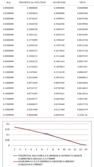
Table 1. Numerical results of problem 1 at H = 0.01.

X(n) THEORITICAL SOLUTION OLUBUNMI TRUN

0.00000000 0.20000000 0.20000000 0.00000000

0.01000000 0.19936034 0.20000000 0.00063966

0.02000000 0.19744547 0.19999953 0.00255406

0.03000000 0.19426760 0.19626706 0.00199946

0.04000000 0.18984708 0.19087657 0.00102949

0.05000000 0.18421221 0.18522314 0.00101093

0.06000000 0.17739899 0,17885647 0.00145748

0.07000000 0.16945103 0.17057349 0.00112246

0.08000000 0.16041915 0.16179043 0.00137128

0.09000000 0.15036115 0.15114648 0.00078533

0.09999999 0.13934135 0.14011432 0.00077297

0.11000000 0.12743023 0.12878653 0.0013563

0.12000000 0.11470401 0.11534238 0.00063837

0.13000000 0.10124406 0.10815221 0.00690815

0.14000000 0.08713649 0.08937685 0.00224036

0.14999999 0.07247157 0.07387969 0.00140812

0.16000000 0.05734305 0.05876521 0.00142216

0.17000000 0.04184773 0.04497863 0.0031309

0.17999999 0.02608475 0.02765649 0.00157174

0.19000000 0.01015490 0.01217869 0.00202379

0.19999999 0.00583989 0.00592321 8.332E−05

(11)

[image:11.595.208.539.89.701.2]

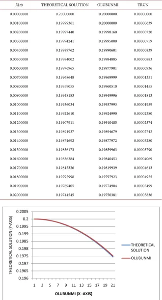
DOI: 10.4236/am.2019.105022 322 Applied Mathematics Table 2. Numerical results of problem 1 at H = 0.001.

X(n) THEORETICAL SOLUTION OLUBUNMI TRUN

0.00000000 0.20000000 0.20000000 0.00000000

0.00100000 0.19999361 0.20000000 0.00000639

0.00200000 0.19997440 0.19998160 0.00000720

0.00300000 0.19994241 0.19995000 0.00000759

0.00400000 0.19989762 0.19990601 0.00000839

0.00500000 0.19984002 0.19984885 0.00000883

0.00600000 0.19976965 0.19977901 0.00000936

0.00700000 0.19968648 0.19969999 0.00001351

0.00800000 0.19959055 0.19960510 0.00001455

0.00900000 0.19948183 0.19949996 0.00001813

0.01000000 0.19936034 0.19937993 0.00001959

0.01100000 0.19922610 0.19924990 0.00002380

0.01200000 0.19907911 0.19910485 0.00002574

0.01300000 0.19891937 0.19894679 0.00002742

0.01400000 0.19874692 0.19877972 0.00003280

0.01500000 0.19856173 0.19859963 0.00003790

0.01600000 0.19836384 0.19840453 0.00004069

0.01700000 0.19815326 0.19819939 0.00004613

0.01800000 0.19792998 0.19797923 0.00004925

0.01900000 0.19769405 0.19774904 0.00005499

0.02000000 0.19744545 0.19750381 0.00005836

(12)

[image:12.595.202.543.88.704.2]

0.00000000 0.10000000 0.10000000 0.0000000

0.00100000 0.09900676 0.09900348 0.00000328

0.00200000 0.09802692 0.09807573 0.00004891

0.00300000 0.09706028 0.09713825 0.00007797

0.00400000 0.09610662 0.09618537 0.00007875

0.00500000 0.09516575 0.09527836 0.00011261

0.00600000 0.09423748 0.09434861 0.00011113

0.00700000 0.09332163 0.09343216 0.00011053

0.00800000 0.09241800 0.09252773 0.00010973

0.00900000 0.09152640 0.09173281 0.00020641

0.01000000 0.09064666 0.09081132 0.00016472

0.01100000 0.08977859 0.08999590 0.00021731

0.01200000 0.08892203 0.08899999 0.00022040

0.01300000 0.08807679 0.08835681 0.00028002

0.01400000 0.08724272 0.08752332 0.00028079

0.01500000 0.08641962 0.08673274 0.00031312

0.01600000 0.08560735 0.08570748 0.00030213

0.01700000 0.08480573 0.08413814 0.00043241

0.01800000 0.08401462 0.08427880 0.00051327

0.01900000 0.08323386 0.08382617 0.00059231

0.02000000 0.08246327 0.08209541 0.00063214

[image:12.595.203.541.90.713.2]

(13)

[image:13.595.199.537.91.697.2]

0.00000000 0.10000000 0.10000000 0.00000000

0.00010000 0.09990007 0.09992720 0.00002713

0.00020000 0.09980027 0.09983454 0.00003427

0.00030000 0.09970061 0.09974292 0.00004231

0.00040000 0.09960109 0.09965531 0.00005422

0.00050000 0.09950170 0.09956093 0.00005923

0.00060000 0.09940244 0.09946347 0.00006123

0.00070000 0.09930332 0.09937088 0.00006676

0.00080000 0.09920434 0.09927559 0.00007125

0.00090000 0.09910548 0.09918759 0.00008211

0.00100000 0.09900676 0.09909777 0.00009101

0.00110000 0.09890819 0.09894247 0.00010113

0.00120000 0.09880973 0.09886919 0.00013274

0.00130000 0.09871142 0.09877561 0.00015777

0.00140000 0.09861323 0.09861727 0.00016238

0.00150000 0.09851518 0.09854087 0.00018621

0.00160000 0.09841727 0.09845110 0.00020000

0.00170000 0.09831949 0.09836652 0.00022135

0.00180000 0.09822183 0.09827469 0.00022927

0.00190000 0.09812431 0.09830139 0.00024221

0.00200000 0.09802692 0.09837561 0.00027725

(14)

In our subsequent research, we shall pay more attention on the implementa-tion of this new scheme to solve some higher order initial value problems of or-dinary differential equation and also compare the results with the existing me-thods and thereafter we examine the characteristics properties such as the stabil-ity, convergence, accuracy and consistency of the scheme.

Conflicts of Interest

The authors declare no conflicts of interest regarding the publication of this paper.

References

[1] Fatunla, S.O. (1987) An Implicit Two-Point Numerical Integration Formula for Li-near and Non-LiLi-near Stiff System of ODEs. Mathematics of Computation, 32, 1-11.

https://doi.org/10.1090/S0025-5718-1978-0474830-0

[2] Ibijola, E.A. (1997) A New Numerical Scheme for the Solution of Initial Value Problem (IVPs). Ph.D. Thesis, University of Benin, Nigeria.

[3] Ibijola, E.A. (1998) On the Convergence, Consistency and Stability of a One-Step Method for Integration of ODEs. International Journal of Computer Mathematics, 73, 261-277. https://doi.org/10.1080/00207169908804894

[4] Obayomi, A.A. (2012) A Set of Non-Standard Finite Difference Schemes for the So-lution of an Equation of the Type _{y y}_{′ =}

(

1₋_yn

)

_._{International Journal of Pure and}

Applied Sciences and Technology, 12, 34-42.

[5] Ogunrinde, R.B. (2010) A New Numerical Scheme for the Solution of Initial Value Problems in Ordinary Differential Equations. Ph. D. Thesis, University of Ado Ekiti, Nigeria.

[6] Ogunrinde, R.B. (2013) On Some Models Based on First Order Differential Equa-tions. American Journal of Scientific and Industrial Research, 4, 288-293.

https://doi.org/10.5251/ajsir.2013.4.3.288.293

[7] Ogunrinde, R.B. and Lebile, O. (2015) On Mathematical Model of Traffic Control.

Mathematical Theory and Modeling, 5, 58-68.

[8] Ogunrinde, R.B. (2016) On Error Analysis Comparison of Some Numerical Expe-rimental Results.