Improved Ostrowski Like Methods Based on Cubic Curve Interpolation

(1)

doi:10.4236/am.2011.27109 Published Online July 2011 (http://www.SciRP.org/journal/am)

Improved Ostrowski-Like Methods Based on Cubic

Curve Interpolation

Janak Raj Sharma1, Rangan Kumar Guha1, Rajni Sharma2

1

Department of Mathematics, Sant Longowal Institute of Engineering and Technology, Longowal, India 2

Department of Applied Sciences, D.A.V. Institute of Engineering and Technology Kabirnagar, Jalandhar, India E-mail: [email protected], [email protected], [email protected]

Received December15, 2010; revised May 10, 2011; accepted May 13, 2011

Abstract

In this paper, we derive two higher order multipoint methods for solving nonlinear equations. The method-ology is based on Ostrowski’s method and further developed by using cubic interpolation process. The adap-tation of this strategy increases the order of Ostrowski’s method from four to eight and its efficiency index from 1.587 to 1.682. The methods are compared with closest competitors in a series of numerical examples. Moreover, theoretical order of convergence is verified on the examples.

Keywords: Nonlinear Equations, Ostrowski’s Method, Root-Finding, Order of Convergence, Cubic Interpolation

1. Introduction

Finding the root of a non-linear equation f x( )0 is a common and important problem in science and engi-neering. Analytic methods for solving such equations are almost non-existent and therefore, it is only possible to obtain approximate solutions by relying on numerical methods based on iteration procedures. Traub [1] has classified numerical methods into two categories viz. 1) one-point iteration methods with and without memory, and 2) multipoint iteration methods with and without memory. Two important aspects related to these classes of methods are order of convergence and computational efficiency. Order of convergence shows the speed with which a given sequence of iterates converges to the root while the computational efficiency concerns with the economy of the entire process. Investigation of one – point iteration methods with and without memory, has demonstrated theoretical restrictions on the order and efficiency of these two classes of methods (see [1]). However, Kung and Traub [2] have conjectured that multipoint iteration methods without memory based on evaluations have optimal order . In particular, with three evaluations a method of fourth order can be constructed. The well-known Ostrowski’s method [3] is an example of fourth order multipoint methods without memory which is defined as

n 2n1

 

i ,

i i i

f x

w x

f x

  

 

1 ,

2

i i

i i i

f w f x

x w

f x f x f w

   _ _ (1)

where i0,1, 2, and x0 is the initial approximation sufficiently close to the required root. The method re-quires two function f and one derivative f evalua-tions per step and is seen to be efficient than classical Newton’s method.

Recently, based on Ostrowski’s method (1) Grau and Díaz-Barrero [4] have developed a sixth order method requiring four evaluations, namely three f and one

f per iteration. Sharma and Guha [5] have shown that there exists a family of such sixth order methods with equal number of evaluations.

In the present paper, we derive two modified Os-trowski’s-type methods which improve the local order of convergence from four for Ostrowski’s method to eight for new methods. The important feature of these methods is that per step they require three evaluations of f and one evaluation of f. Thus, the new methods support the conjecture of Kung and Traub for eighth order methods based on four evaluations.

(2)

effi-J. R. SHARMA ET AL. 817 ciency of the methods is discussed. Section 4 contains

the numerical experimentations and comparison with some well known methods. Concluding remarks are given in Section 5. In Section 6, references are given.

2. The Methods and Their Convergence

Method One

Consider the Ostrowski scheme (1) now defined by

 

,

. 2 i

i i i

i i

i i i

f x

w x

f x

f w f x

z w

f x f x f w

    

 

(2)

In what follows, we construct the method to obtain the approximation xi1 to the root by considering the cubic curve interpolation. Let

 



 



2





3

,

i i

y x  a b xx c xx d xxi (3) be an interpolatory polynomial of degree three such that

 

_i

 

_i ,

y x  f x (4)

 

_i

 

_i ,

y x  f x (5)

 

_i

 

_i ,

y w  f w (6)

 

_i

 

_i ,

y z  f z (7) and

 

_i

 

_i .

y z  f z (8) Our interest is to find the unknown parameters a, b, c and d introduced in the polynomial. In order to achieve that, we make use of the expressions (4) - (7) in (3). From (3), (4) and (5), it is easy to show that

 

( ),

.

i

a f x

b f x

 

 (9)

Substituting the values of a and b in (3) then using (6) and (7), we obtain after some simple calculations

( ) ( )

1

( ) i i ( )

i i i

i i i i

f w f x

c d w x f x

w x w x

  _ 

   _  _

 _  _, (10)





1

 

.

i i

i i i

i i i i

f z f x

c d z x f x

z x z x

  



   _  _

 _  _ (11)

Solving these equations using Ostrowski iteration (2), we obtain

 

   

 

2

,

i i i

i

i i i i

f x f x f w

c f w

f x f w f x f w



 

  

 

 

_{   }

 

_

 

_{ }

_

3

3 2

2

,

i i i

i _i _i _i

f x f x f w

d H

f x _{f w} _{f x} _{f w}

 



 (13)

where

     



 





 



 







 



3

2

2 .

i i i i i i

i i i i

H f x f w f x f w f x f w

f x f z f x f w

  

  



.

The tangent line to the curve of cubic polynomial (3) at the point



z y zi,

 

i



is given by

 

_i

 

_i _i



.

yy z y z xz (14) Assuming that the root estimate xi1 is point of inter-section of the tangent line (14) with x-axis, then

 

i 1 0.

y x_  Thus, from (7), (8) and (14), we obtain

 

1 .

i i i

i

f z

x z

y z

   _ (15)

Now using the approximation (8) in (15), we can ob-tain the new improvement as given by

 

1 .

i i i

i

f z

x z

f z

   _ (16)

where i is the Ostrowski point. It is quite obvious that formula (16) together with (2) requires five evaluations per iteration. However, we can reduce the number of evaluations to four by utilizing the approximation (8). Therefore, (3) and (8) yield

z

 









2

2 3

i i i i i i

f z y z  b c z x  d z x . (17) Substituting the values of c and in (17), we obtain

,

b d

 

_i

 

_i



_i



,

f z y z f x (18) where

   



 



     



 





 



   



 





 



     



 





 



3

2

1

2 2

2

2 .

i i i i i i

i i i i i

i i i

i i i i i i

f w f w f x f x f z f w

f x f x f w f w f z

f x f x f w

f x f w f w f x f x f w

 





_ 

  



  _

 

_   _

Then the formula (16) in its final form is given by

 

1

 

_{ }

1 ,

i i i

i

f z

x z

f x

 

   _ (19)

where zi is the Ostrowski iteration (2) and  is given in (18).

2H    (12)

(3)

util-izes four pieces of information namely- f x

 

_i , f

 

x_i ,

 

i

f w and f z

 

_i . Since we are using the approxima-tion (8) for the derivative, therefore the error is given by (see [6])

Theorem 1. Let f x

 

be a real valued function. As-suming that f x

 

is sufficiently smooth in an interval I. If f x

 

has a simple root I and x0 is suffi-ciently close to  then the method defined by (19) is of order eight.

 

  

 

2

, 4!

iv

i i i i i

f

f z y z   z x z w_i





(20) where  min



x w z_i, _i, _i



, max



x w z_i, _i, _i _. In order to show that the method is of order eight, we prove the fol-lowing theorem:

Proof: Let e_i x_i , e_iw_i and eˆ_i z_i 

be errors in the ith iteration. Using Taylor’s series expan-sion of f x

 

i about  and taking into account that

 

f  0 and f

 

 0, we have

 

2 3 4 5 6

 

7

2 3 4 5 6 ,

i i i i i i i

f x  f  _e A e A e A e A e A e O e_i _ (21) where 1 !A_k 



k



f k

   

 f  , k2, 3, Furthermore, we have

 

2 3 4 5

 

6

2 3 4 5 6

1 2 3 4 5 6

i i i i i i

f x  f  _  A e  A e  A e  A e  A e O e_i _. (22)

 



 





2 2 3 3 4 2 2

2 3 2 4 3 2 2 5 4 2 3 3 2 2

2 2 3 5 6 7

6 5 2 4 3 4 2 3 2 3 2 2

2 3 7 4 4 10 6 20 8

5 13 17 28 33 52 16 .

i

i i i i

i

i i

f x

e A e A A e A A A A e A A A A A A A e

f x

A A A A A A A A A A A A e O e

           



       



 

4 5

i

(23)

Substitution of (23) in first step of (2), yields



 







2 2 3 3 4 2 2

2 3 2 4 3 2 2 5 4 2 3 3 2 2

2 2 3 5 6 7

6 5 2 4 3 4 2 3 2 3 2 2

2 3 7 4 4 10 6 20 8

5 13 17 28 33 52 16 .

i i i i

i i

e A e A A e A A A A e A A A A A A A e

A A A A A A A A A A A A e O e

          

       



 

4 5 i

(24)

Expanding f w

 

i about  and using (24), we obtain

 



 







 

2 2 3 3 4 2 2

2 3 2 4 3 2 2 5 4 2 3 3 2 2

2 2 3 5 6 7

6 5 2 4 3 4 2 3 2 3 2 2

2 3 7 5 4 10 6 24 12

5 13 17 34 37 73 28 .

i i i i

i i

4 5

i

f w f A e A A e A A A A e A A A A A A A e

  

 _          



        _ (25)

Using Equations (21), (23) and (25), we obtain

 



 





2 2 3 3 4 2 2

2 3 2 4 3 2 2 5 4 2 3 3 2 2

2 2 3 5 6 7

6 5 2 4 3 4 2 3 2 3 2 2

2 2 3 6 3 4 8 4 12 4

2

5 10 10 16 15 22 6 .

i i

i i i

i i

f x f w



 

4 5

i

A e A A e A A A A e A A A A A A A

f x f x f w

          

 

       

e

(26)

From second step of (2) it follows that



 







3 4 2 2 4 5

2 3 2 4 2 3 3 2 2

2 2 3 5 6 7

5 2 4 3 4 2 3 2 3 2 2

ˆ 2 2 8 4

3 7 12 18 30 10 .

i i i

i i

e A A A e A A A A A A e

 

A A A A A A A A A A A e O e

      

        (27)

Expanding f z

 

_i about , we obtain

 

2

 

9

2

ˆ ˆ ,

i i i

(4)

J. R. SHARMA ET AL. 819

 



 







3 4 2 2 4 5

2 3 2 4 2 3 3 2 2

2 2 3 5 6 7

5 2 4 3 4 2 3 2 3 2 2

2 2 8 4

3 7 12 18 30 10 .

i i i

i i

f z f A A A e A A A A A A e

A A A A A A A A A A A e O e

  

 _      



       

 

_

2 ,

(29)

Using the results of (21), (25) and (29) in

   



 



     



 





 



   



 





 



     



 





 



3

1 2

2

2 2

i i i i i i i i i

i i i i i i i i i i i

f w f w f x f x f z f w f x f x f w

f w f z f x f x f w f x f w f w f x f x f w

 

 

_   

  

   _{ }   _

and simplifying, we get



2

 

2 3

 

3 2 2 4



4



2 2 3 4 3 2 2 5 4 2 3 3 2 2

1 2A e_i 4A 3A e_i 4A 12A A 8A e_i 5A 17A A 9A 38A A 18A e_i O e_i5



.

             

(30)

From (22) and (30), we get

 



3



4

 

5

2 4 3 2 2

1 2 2

i

f x f A A A A A e O e

     _    _i  _i _. (31)

Using (28) and (31) in

 

1

1 ,

i i i

i

f z

x z

f x

 

   _ we find the error equation as given by

 





 









 











 

2 9

2 ₂ ₃

1 ₃ ₄ ₅ 2 2 4 3 2 2

2 4 3 2 2

2 3 4 9

2 2 4 3 2 2

2

3 3 3 8 9

2 2 3 2 2 4 3 2 2 2 3 2

2 2

ˆ ˆ

ˆ ˆ ˆ ˆ 1 2 2

1 2 2

ˆ 2 2 ˆ

2 2

i i i

i i i i i i i

i i

i i i i

i i

e A e O e

e e e e A e A A A A A e O e

A A A A A e O e

A e A A A A A e e O e

A A A A A A A A A A A A e O e

A A 

   

  _ __ _

   _  _{ }    _

     

 

 

 _    _

 

 _      _ 

 





2

 

2



8

 

9

2A3 A2 A2A3 A e4 i O ei .

 

4 9

(32)

Thus Equation (32) establishes the maximum order of convergence equal to eight for the iteration scheme de-fined by (19). This completes the proof of the theorem.

Remark 1. The error (20) is now given by

 

  

 

2



ˆ ˆ .

4! iv

i i i i i i

f

f z y z   e e e e

From (24), (27) and Taylor’s expansion of f iv

 

 about , we can obtain the error as

 

4

 

5

4 2 .

i i i i

f z y z  A A e O e (33) This shows that the error in derivative approximation is of order four.

Remark 2. Upon using Taylor’s expansion

 

i

f z 

 

2

2ˆ ˆ

1 2 i i

f  _  A e O e _

i 

 

_,

in (33), we get

 

4

 

5

2ˆ 4 2

1 2 ,

i i i

y z  f  _  A e A A e O e that is

 



3



4 5

2 4 3 2 2

1 2 2

i

i i

y z

f  A A A A A e O e



 



 _     (34)

which is same as obtained in equation (31) of

 

_i

 

_i .

y z f x This verifies the correctness of error (33) and calculation of y z

 

i .

Remark 3. From the convergence theorem of iterative functions [1], if g1

 

x and g2

 

x

p

 

are two iterative functions of order 1 and 2, respectively, then the new composite iterative function

p

 



2 1 g g x





G x

i z

has the order 1 2 In our case, the Ostrowski method (2) comprising the first two steps, is of order four. Thus to produce eighth order method the formula (19) should be of order two (neglecting how is obtained). From (34), it turns out that

. p p

 

1

 

e .

ˆ A eˆ

ˆ

f O

   

3 i f xi

   

 

2

ˆ . O e

i

 

Also, the Taylor’s series expansion of the

func-tion i i 2 i i

y z

 

e

 

f

f z    _   _ On substitution and simplifying, we see that the Newton-like method (15) and hence (19), has the order two, thus verifying the con-vergence theorem on composition of two iterative func-tions to produce eighth order iterative method.

2.2. Method Two

(5)



 







 



 



 





2 3 , i i i

F f x A B f x f x

C f x f x

D f x f x

  

 

(35)

be an inverse interpolatory polynomial of degree three such that

 



_i



_i,

F f x x (36)

 



i



 

i 1,

F f x f x  (37)

 



_i



_i,

F f w w (38)

 



_i



_i,

F f z z (39)

and

 



i



 

i 1.

F f z f z  (40) From (36) and (37), we can calculate A and as given by

B

 

, 1

i i .

Ax B f x (41) Substituting the values of A and in (35), then using (38) and (39), we obtain

B

 





 





2

 

1

i i

i

i i

C D f w f x

f w

f x

f w f x

      (42) and

 





 





 

2 1 . 2 i i i i

i i i

i i i i

C D f z f x

f z f x

f w f x f z

f x f x f w f x

        _ _  _      (43)

The Equations (42) and (43) when solved, yield

 





 

2 1 1 , i i i i i i

i i i

f w C

f x

f w f x

G

f x f w f z

        (44)

   



1

 



,

i i i

D G

f x f w f z



  (45) where      





   





          2 2 1 . 2 i i i i i i i i i i f w G

f w f x

f x f w f z

f x f w

f z f x               

The tangent line to the curve of cubic polynomial (35) at the point



F f z



 

i



,f z

 

i



is given by

 







 

i





 

i





 

i



. F f x F f z F f z f x  f z The approximation to the root xi1 is now obtained by intersecting this tangent line with x-axis. This yields

 

1 , i i i i f z x z f z

   _ (46)

where

 



 



 





 





₂ 1

1 2 3 . i i i i i i

f z F f z

B C f z f x

D f z f x

     _      _

From (40), (44) and (45), we have

 

1 1

,

i i

f z  f x (47)

where

 

_{ }

   

_{ }

2 1 1 2 . 2 i i

i i i i

i i

i

i i

f w f z f x

f w f z f w f z

f w f z f z f x

f x f w

f z

f w f w

   _  _      i              _  _     

Hence, the iteration formula (46) is given by

 

1 , i i i i f z x z f x 

   _ (48)

where zi is the Ostrowski iteration (2) and  is shown in (47).

Thus, we obtain second modified Ostrowski-like method (48) developed by tangential inverse interpolation. In this method also, the number of evaluations required is same as in the first method. Error in the approximation (40), likewise the error (20), can be given by

 



 



     







 



( ) 2 1 , 4! i i iv

i i i i

F f z

f z

f

f z f x f z f w

       (49) where

     





     





min , , ,

max , , .

i i i

f x f w f z

_{ }

(6)

J. R. SHARMA ET AL. 821 In the following theorem we prove that the method is

of order eight.

Theorem 2. Under the hypotheses of theorem 1, the

it-eration method defined by (48) is of order eight.

Proof: Using (21), (25) and (29), after simple calcula-tions we find

 

   

 



2



2





3



2 4



4 5

2 3 2 4 3 2 5 4 2 2 3 2

1 2

2

1 4 6 2 8 4 10 6 2 2 .

i i i

i i i i i i

i i i i

f w f x f z

f w f z f z f x f x f w

 

i

A e A A e A A A e A A A A A A e O e

   

 

 _ _   _ 

   

   

          

(50)

Also

 













2

2 2 3 2 4 4 5

2 3 2 4 3 2 6 4 2 2 3 2

1 2 3 2 4 4 5 .

i i i

i i i i

f w f z f x

f w f z f w f x

 

i

A e A A e A A A e A A A A A A e O e

  

 

 __  __

          

(51)

From (47) we know   1 Equation (50) Equation (51) , which implies







2 3 2 4 4

2 3 4 5 4 2 3 2 2

1 2_{A e}_i 3_{A e}_i 4_{A e}_i 5_A _{A A} 7_{A A} 7_A _e_i _{O e}_i5



.

          (52) From (22) and (52), we get

 

2



4 3 2 23



4

 

5

1

1 7 7 _i _i

i

A A A A A e O e

f x f .



  

 _      _

  (53)

Then using (28) and (53) in

 

1 ,

i i i

i

f z

x z

f x



   _ we obtain the error equation

 





 





 





 











2 9 2 4 4 5

1 2 4 2 2 3 2

2 2 4 4 9

2 4 2 2 3 2

2 3 4 9

2 2 4 3 2 2

2

3 3 3

2 2 3 2 2 4 3 2 2 2 3 2

ˆ ˆ ˆ 1 7 7

ˆ 7 7 ˆ

7 7

i i i i i i i

i i i i i

i i i i

i i

e e e A e O e A A A A A e O e

e e A e A A A A A e O e

A e A A A A A e e O e

8

A A A A A A A A A A A A e O e

  _    _{ }     

 

 _  _{ }     _

 

 _     _

 

 _       _ 

 

 

 









 

9

2 2 2 8 9

2 2 3 6 2 2 3 4 i i .

A A A  A A A A e O e

  _   _ 

(54)

This result shows the eighth order convergence of method (48).

Remark 4. The error (49) upon using (21), (25) and (29) is given by

 



 



 

_{ }

 





3 ₄

 

₅

2

1

. 4!

i i

iv

i i

F f z

f z

F

f A e O e





  

 _ 

 __  __

Expanding F iv

 

 about  and using the fact that

 





 





   

 





 

_{ }

 





 





3 ( )

7 6 5

3

2 3 2 4

4

15 10

(0)

4!

5 5 ,

iv

iv f f f f

F

f f f

A A A A

f

   

  

 

  

  

  

 

 _   _



we can obtain the error as

 



 



 

2 4 3 2 23 4

 

5 1

1

5 5

i i

F f z f z

.

A A A A A e O e f 

  

 

 _ _   _ 

(55

in approximation (40) is of or

Remark 5. Upon using Taylor’s expansion

)

This shows that the error der four.

 

1 f zi

 

2

2ˆ ˆ 1 f  1 2A ei O ei 

_ _{ }   _in (55), we get

 





 



3



4

 

5

1

ˆ

1 2A e A A 5A A 5A e O e ,

 2 2 4 3 2 2

i

i i i

F f z

f

 

 _       _

(7)

 





 

2



4 3 2 23



4 5

1

1 7 7

i

i i

F f z

A A A A A e O e

f 

 

 _     

 

,



which is same as obtained in Equation (53) of



 



i



 

i .

F f z  f x This verifies calculations of rm (55) and

error te F



f z

 

i



.

Remark 6.

Since F



f z

 

i



 f

 

xi 1 f

 

  1O

 

ˆ , therefore, similar to remark 3, the iterative formula (48) combined with the Ostrowski iteration (2) verifies the iterative functions to produce eig

3. Computational Efficiency

i e

convergence theorem on composition of two hth order iterative method.

In order to obtain an assessment of the efficiency of our methods we shall make use of Traub’s efficiency index ([1], Appendix C), according to which computational efficiency of an iterative method is given by _E__p1c

, where

p

is the order of the method and c is the cost per ction and derivative

at is, iterative step of computing the fun

required by the iterative formula, th c



cj, cj is the cost of evaluating f j for j0. The value

0

j simply gives the function f .

Designating Ostrowski’s method (1) as M4, sixth order method [4] as M6 and present methods (19) and (48) as M8,1 and M8,2, respectively. Assuming that the cost of evaluating f j is 1, then for M8 we find efficiency index 1 4

8 1.682.

E  For M6 ,

1 4 6 1.565

 and similarly for

E 4,

M 1 3

4 esent m

1

h r ethods are .587.

E  Com-

the E values we find that t e p paring

better options than both of M4 and M6.

4. Numerical Illustrations

In this section, we apply the modified methods M8,i



i1, 2



to solve some nonl ar equa ich not only illustrate the methods practically but also serve to check the validity of theoretical results we have derived. The performance is comp 4

ine tions, wh

ared with M and M6. In mes order to compare the higher ord

necessary that we use higher pre

er m s it

cision in computations. pre-ethod beco

Therefore, the calculations are performed with high-cision arithmetic and terminated after three iterations. To check the theoretical order of convergence, we obtain the computational order of convergence (p) using the formula (see [7])



 





1

 

1



ln

. ln

i i

x x

p

x x

 





 



[image:7.595.305.533.91.715.2]

 

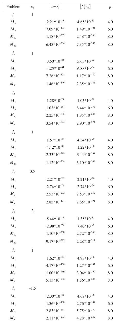
Table 1. Performance of methods.

Problem x0 ax3 f x 3 p

1

f 1

4

M 2.21*10–34_4.65*10–33_4.0

6

M 7.09*10–103_1.49*1₀–101_6.0

8,1

M 1.18*10–269_2.48*10–268_8.0

8,2

M 6.43*10–204_7.35*10–202_8.0

2

f 1

4

M 3.50*10–22 5.63*10–22 _4.0

6

M 4.25*10–64_6.83*10–64_6.0

8,1

M 7.26*10–171_1.17*10–170_8.0

8,2

M 1.46*10–146_2.35*10–146_8.0

3

f

4

M 1.28*10–78 1.05*10–78 4.0

6

M 1.03* 0₁ –251_{8.44* 0}₁ –252_6.₀

8,1

M 2.25*10–635_1.85*10–635_8.0

8,2

M 3.54*10–574 2.90*10–574 8.0

4

f 1

4

M 1.57*10–29 4.34*10–29 4.0

6

M 4.42*10–81_1.22*10–80_6.0

8,1

M 2.33*10–298_6.44*10–298_8.0

8,2

M 1.12*10–209 3.10*10–209 8.0

5

f 0.5

4

M 2.21*10–26_2._21*10–26_4.0

6

M 2.74*10–76_2.74*10–76_6.0

8,1

M 2.53*10–232_2.53*10–232_8.0

8,2

M 2.85*10–191_2.85*10–191_8.0

6

f 2

4

M 5.44*10–32_1._35*10–31_4.0

6

M 2.98*10–95_7.40*10–95_6.0

8,1

M 1.10*10–268_2.72*10–268_8.0

8,2

M 9.17*10–212_2.28*10–211_8.0

7

f 1

4

M 1.62*10–36_4._93*10–36_4.0

6

M 4.17* 01 –108 1.27* 01 –107 6.0

8,1

M 1.00*10–269_3.04*10–269_8.0

8,2

M 5.13*10–236_1.56*10–235_8.0

8

f –1.5

4

M 2.30*10–39_4.68*10–38_4.0

6

M 1.36* 0₁ –108_{2.76* 0}₁ –107_6.₀

8,1

M 2.83*10–231 5.75*10–230 8.0

8,2

M 2.11*10–233_4.28*10–232_8.0

(8)

J. R. SHARMA ET AL. 823

 





 

2

1, 



 



 

3 2

1

5 2

2

3

4

3 5

2 6

7

1 319 636

0.3459 482420

sin 2 , 1.8954942670339809,

10 exp 1.6 4284 ,

g 1 ,

sin 1.40 8 1534

cos

f x x

f x x x

f x x

f x x x

f x x



   

  

 

  

 

2 ₂

8

, 0.51775736368245830,

sin 3cos 5,

1.2076478271309189.

x

xe

f x xe x x



 

   

 

Table 1 shows the absolute difference



, 0

x  

 

x 2__1, _

4x 5,  1.6 808055660 ,

1 ,  548158 ,

79630610 499

lo

449164 2 12,

x 

 

   

3

x

 , the absolute value of the function f x

 

3

). It can be obs blems, t

and the computa-tional order of convergence (p erved clearly that in all considered test pro he new methods

8,i

M



i1, 2



4

compute the results with higher precision than M and M6. This superiority of M8,i agrees

is of order and effici scussed in previous sections.

5.

the p int iterat

q alua

with theoretical analys ency di

Conclusions

In this work, we have obtained two multipoint methods of order eight using an additional evaluation of function at o ed by Ostrowski’s method of order four for solving e uations. Thus, one requires three ev tions of the function f and one of its first-derivative f per full step and therefore, the efficiency of the me s

ki’s method. The superiority of pre-orated by numerical resul displayed in the table 1. The computational order of

con-ro

of One-Point and Multipoint Iteration,” Journal of the Association for chinery, Vol. 21, No. 4, 1974, pp. 643-651.

thods i better than Ostrows

sent methods is also corrob ts

vergence (p) overwhelmingly supports the eighth order

convergence of our methods. These methods also p vide the examples of eighth order methods requiring four evaluations for Kung and Traub conjecture. Finally, we conclude the paper with the remarks that such higher or-der methods are useful in the numerical applications re-quiring high precision in their computations.

6. References

[1] J. F. Traub, “Iterative Methods for the Solution of Equa-tions,” Prentice Hall, Englewood Cliffs, 1964.

[2] H. T. Kung and J. F. Traub, “Optimal Order

Computing Ma

doi: 10.1145/321850.321860

[3] A. M. Ostrowski, “Solutions of Equations and System of Equations,” Academic Press, New York, 1960.

[4] M. Grau and J. L. Díaz-Barrero, “An Improvement to Ostrowski Root-Finding Method,” Applied Mathematics and Computation, Vol. 173, No. 1, 2006, pp. 450-456. doi:10.1016/j.amc.2005.04.043

[5] J. R. Sharma and R. K. Guha, “A Family of Modified Ostrowski Methods with Accelerated Sixth Order Con-vergence,” Applied Mathematics and Computation, Vol. 190, No. 1, 2007, pp. 111-115.

doi:10.1016/j.amc.2007.01.009

[6] G. M. Phillips and P. J. Taylor, “Theory and Applications

ers, Vol. 13, No. 8, 2000, of Numerical Analysis,” Academic Press, New York, 1996.

[7] S. Weerakoon and T. G. I Fernando, “A Variant of New-ton’s Method with Accelerated Third-Order Conver-gence,” Applied Mathematics Lett