Bayesian Estimations with Fuzzy Data to Estimation Inverse Rayleigh Scale Parameter

(1)

http://www.scirp.org/journal/ojapps ISSN Online: 2165-3925

ISSN Print: 2165-3917

DOI: 10.4236/ojapps.2019.98054 Aug. 29, 2019 673 Open Journal of Applied Sciences

Bayesian Estimations with Fuzzy Data to

Estimation Inverse Rayleigh Scale Parameter

Shurooq Ahmed Kareem AL-Sultany

Department of Mathematics, College of Science, Mustansiriyah University, Baghdad, Iraq

Abstract

In this paper, Bayesian computational method is used to estimate inverse Ray-leigh Scale parameter with fuzzy data. Based on imprecision data, the Bayes es-timates cannot be obtained in explicit form. Therefore, we provide Tierney and Kadane’s approximation to compute the Bayes estimates of the scale parameter under Square error and Precautionary loss function using Non-informative Jefferys Prior. Also, we provide compared numerically through Monte-Carlo simulation study to obtained estimates of the scale parameter in terms of mean squared error values.

Keywords

Inverse Rayleigh Distribution, Imprecision Data, Modified Newton Method, Tierney and Kadane’s Approximation

1. Introduction

The Rayleigh distribution (RD) is originated from two parameter Weibull distri-bution and it is an appropriate model for life-testing. It can be shown by transfor-mation of random variable that if the random variable X has Rayleigh distribution, Then the random variable Y 1

X

= _{has an inverse Rayleigh distribution (IRD)}

[1]. The Inverse Rayleigh distribution (IRD) has been introduced by Trayer (1964) [2]. The distribution of life times of several types of experimental units can be approximated by the IRD [3]. The IRD plays an important role in many applications, including life test and reliability studies [4]. A random variable Y is said to have a one-parameter (IRD) if it has the following (PDF),

(

)

2

3

2

; ey ; 0, 0

Y

f y y

y

λ

−

= ≥ > ₍₁₎

How to cite this paper: AL-Sultany, S.A.K. (2019) Bayesian Estimations with Fuzzy Data to Estimation Inverse Rayleigh Scale Parameter. Open Journal of Applied Sciences, 9, 673-681.

https://doi.org/10.4236/ojapps.2019.98054

Received: July 28, 2019 Accepted: August 26, 2019 Published: August 29, 2019

http://creativecommons.org/licenses/by/4.0/

(2)

DOI: 10.4236/ojapps.2019.98054 674 Open Journal of Applied Sciences and (CDF), is given by:

(

)

2

; ey ; 0, 0

Y

F y y

λ

λ λ

−

= ≥ > ₍₂₎

where λ_{is the scale parameter.}

2. Maximum Likelihood Estimators (MLE)

Given y=

(

y1,y2,,ym

)

be an (i.i.d.) random vector of a random sample of size m from (IRD), the complete-data likelihood function is:

( )

1 2

1 3 1

1

; 2 e

m i

i

y

m m

i m i

L

y y

λ

=

λ

∏

₌ − ∑= ₍₃₎

Now if y is not observed precisely. Then, we can compute its probability by using Zadeh’s definition of an imprecision event [5]. The observed-data log-likelihood function can then be obtained as,

( )

(

)

( )

1

; ; d

i

m

Y y

i

L

λ

y f y

λ µ

f y y

=

∏∫

_



( )

2

( )

3 1

2

; e _i d

m y

y i

L f y y

y y

λ

λ µ

−

=

∏∫

_

 (4)

where µfy_i

( )

y is the Borel measurable membership function.

Now, by take the natural logarithm for the likelihood function and differen-tiating with respect to λ and then equating to zero we get:

( )

2

5

1 3

1

e d

ln ;

0 1

e d

i

y y m

i

y y

f y y

L _m _y

f y y y

y

λ

µ λ

λ λ

µ

−

− =

∂

= − =

∂

∫

∑

∫



(5)

Since, the (MLE) of λ_{is the solution of Equation (5), so, we used the} mod-ified Newton’s Method to determine the MLE of the parameter λ_.

Where, at iteration

(

h+1

)

( ) ( )

_{( )}

( )

ˆ 1

2 2

ˆ

ln ;

ˆ ˆ _, ₁

ln ;

h

h h

y

y L

L

λ λ

+ =

=

∂ ∂

= − >

∂ ∂



υ υ ₍₆₎

and

( )

2 2

2

2 ₇ ₅

2 2

1 1

3 3

1 1

e d e d

ln ;

1 1

e d e d

i i

y y

m n

i i

y y

f y y f y y

L _m _y _y

f y y f y y

y y

y

λ λ

µ µ

λ

λ λ

µ µ

− −

= =

 

 

∂ _ _

= − + − _ _

∂ _ _

 

 

∫

∑

∫

 



(7)

3. Bayes Estimator

(3)

DOI: 10.4236/ojapps.2019.98054 675 Open Journal of Applied Sciences Bayesian opinion the parameter itself is considered as a random variable from a given probability distribution whose variability can be described by the prior distribution.

Assume that the prior distribution of the unknown scale parameter λ_of IRD defined as using Jeffery’s prior information π λ

( )

, which is given by [2]:

( )

I

( )

π λ

∝

λ

where

( )

(

)

2 2

ln f y;

I λ m E λ

λ

∂ 

= −  

∂

 

 

( )

2

(

2

)

ln f y;

a mE λ

π λ

λ

∂ 

⇒ = − _ _

∂

 

 , a is a constant,

where

(

)

_{( )}

2

2 2

ln ; 1

, 0

f y a m

E λ π λ λ

λ

λ λ

∂ ₌ − _⇒ ₌ _>

 _∂ 

 

 

Now, the posterior density function of λ_{given imprecision data is:}

( )

0

; |

; d y L h

L y

y

π λ

λ

π λ

λ

∞

=

∫

 



( )

2

3 1

3 1 0

2

e d

|

2

e d

i

m y

y i

m y

y i

a m

f y y y

h

a m y

f y y y

λ

λ _µ

λ λ

λ _µ

λ

−

=

− ∞

=

⇒ =

∏ ∫

∏

∫



 (8)

In this study we consider non-informative prior density for λ based on square error and precautionary loss function as the following:

3.1. Bayes Estimator Based on Square Error Loss Function

Bayes estimation of any function of the scale parameter λ_say g

_{( )}

λ , based on a squared error loss function, may be written as,

( )

( ) ( )

( )

0

; d

ˆ |

; d

s

y

y g L

g E g

L y

λ π λ λ λ

λ λ

π λ λ λ

∞

 

= _ _=

∫

 

 (9)

3.2. Bayes Estimator Based on Precautionary Loss Function

Precautionary loss function was proposed by Norstrom (1996) [6], as follows:

( ) ( )

2

ˆ ˆ,

ˆ L

θ θ θ θ

θ −

= ,

where _θˆ_{is an estimate of}_θ_.

(4)

DOI: 10.4236/ojapps.2019.98054 676 Open Journal of Applied Sciences

( )

( ) ( )

( )

2

2 0

0

; d

ˆ |

; d

p

g L y

y

g E g

L y

λ π λ λ λ

λ λ

π λ λ λ

∞

 

= _ _=

∫

 

 (10)

Note that, Bayes estimator in (9) and (10) cannot be simplified in to a closed form. Therefore, we consider Tierney and Kadane’s approximation form to ob-tain Bayes estimator of λ_{of IRD.}

4. Tierney and Kadane’s Approximation Form

Tierney and Kadane (1986) [7] proposed an alternative method for the evalua-tion of the ratio of integrals of the form (9) and (10).

Setting Q

( )

λ

=ln

(

π λ

( )

)

+ln

(

L

( )

λ

;y

)

( )

0

( )

_{( )}( )

0

e d

ˆ |

e d

Q

s y _Q

g

g E g

λ

λ λ

λ

∞

 

= _ _=

∫

 (11)

( )

2

( )

0 2

( )

_{( )} ( )

0

e d

ˆ |

e d

Q

p

Q

g

g E g y

λ

λ λ

λ

∞

 

= _ _ =

∫

 (12)

Now, set

( )

Q

( )

H

m

λ

=

( )

(

( )

)

( )

* ln

s

g

H H

m λ

λ = + λ ₍₁₃₎

And

( )

(

2

( )

)

( )

* ln

p

g

H H

m λ

λ = + λ (14)

( )

0 _{( )}( ) 0

e d

ˆ

e d

s

nH

s _nH

g

λ

λ λ

λ

∗

∞

⇒ =

∫

(15)

( )

_{( )}( )

1 2 0

0

e d

ˆ

e d

p

nH

p

nH

g

λ

λ λ

λ

∗

∞

 

 

=_ _

 

 

∫

(16) Now, the Equation (15) and Equation (16) can be written as

( )

*

{

(

( ) ( )

_ˆ* _ˆ

)

}

ˆ exp s

T s

g λ τ n H λ H λ

τ ∗

= − ₍₁₇₎

( )

*

{

(

( ) ( )

_ˆ* _ˆ

)

}

ˆ exp p

T p

g

λ

τ

n H

λ

H

λ

τ

∗

= − ₍₁₈₎

where,

τ

*_{: is the minus the inverses of the second derivative of}

( )

s

H∗ λ or

( )

p

(5)

( )

s

H∗ λ and Hp

( )

λ

∗ _{as well as}

_λ

_ˆ_maximize

_{( )}

H λ Now, the function H

( )

λ is given by,

( )

(

) ( )

2

( )

3 1

1 1

1 ln ln e d

i

m y

y i

H k m f y y

m y

λ

λ λ µ

− =     = + − +  



∑

∫

  (19)

where,

( )

1

( )

ln ln 2 ln

2

k= a +m + m (20)

and

_λ

ˆ_{that maximize} _H

( )

_λ _{, can be obtained by solving the following} equa-tion,

( )

2 2 5 1 3 1 e d 1 1 0 1 e d i i y y m i y y

f y y

H m y

m

f y y

y λ λ µ λ λ λ µ − − =     ∂ ₌  − ₋ ₌   ∂ _ _    

∫

∑

∫

  (21)

It is clear there is no explicit solution to Equation (21). Therefore, modified Newton method is applied to solve the required equation.

( ) ( )

_{( )}

( )

( ) ˆ 1 2 2 ˆ

ˆ ˆ h _, ₁

h h h H H λ λ λ λ λ λ λ λ λ λ + = = ∂ ∂

= − >

∂ ∂

υ υ ₍₂₂₎

where

( )

(

)

( )

2 2 2 2 2 ˆ ˆ

2 7 5

ˆ ˆ

2 2

1 1

3 3

1 1

e d e d

1 1

e d e d

i i i i y y y y m m i i y y y y

f y y f y y

H m y y

m

f y y f y y

y y λ λ λ λ µ µ λ λ λ µ µ − − − − = =  _ _   _ _    ∂ − −   =  + − _ _  ∂  _ _   _ _       

∫

∑

∫

    (23) then,

( )

( ) 1 2 2 ˆh H λ λ λ τ λ − = _∂  = −   ∂    

Now, following the same argument with g

( )

λ =λ

4.1. Tierney and Kadane’s Approximation of

λ

Based on Square

Error Loss Function (TKS)

Set

( )

λ =λ, Equation (13) will be,

( )

ln

( )

s H H m

λ

∗ ₌ ₊

( )

( ) ( )

2

( )

3 1

1 1

ln ln e d

i

m y

y

s i

H k m f y y

m y

λ

λ λ µ

−

=

∗ ₌ _ ₊ ₊ _

 

(6)

DOI: 10.4236/ojapps.2019.98054 678 Open Journal of Applied Sciences where k is a constant as in (20).

Now,

λ

_ˆ*_{that maximize}

( )

s

H∗ λ in (24) can be obtained by solving follow-ing equation iteratively as in

( ) ( )

_{( )}

( )

( ) ˆ 1 2 2 ˆ

ˆ ˆ h _, ₁

h s s h h H H λ λ λ λ λ λ λ λ λ λ ∗ ∗ ∗ ∗ + ∗ ∗ = = ∂ ∂

= − >

∂ ∂

υ υ ₍₂₅₎

where

( )

* 2 * 2 ˆ 5 ˆ * 1 3 1 e d 1 ˆ 1 e d i i y y m i y s y

f y y

H m y

m

f y y y λ λ µ λ λ λ µ − − = ∗     ∂   = _ − _ ∂ _ _    

∫

∑

∫

 

( )

* * 2 2 * * 2 2 2 ˆ ˆ

2 7 5

2 2 ˆ ˆ

1 1

3 3

1 1

d e d

1 ˆ

1 1

e d e d

i i

y y

s m m

i i

y y

e f y y f y y

H m y y

m

f y y f y y

y y λ λ λ λ µ µ λ λ λ µ µ − − ∗ ₌ − ₌ − ∗  _ _   _ _   _ _  ∂ −   = + −   ∂  _ _   _ _   _ _   

∫

∑

∫

    And

( )

( ) 1 2 * 2 ˆ h s H λ λ λ τ λ ∗ − = ∗ _∂  = −   ∂  

  (26)

Now, Bayes estimate of λ_{of IRD based on square error loss function,} de-noted by ˆTK

s

λ , can be obtained from Equation (17), where all the H and Hs ∗

elements are evaluated in

_λ

ˆ_and

λ

_ˆ*_{respectively.}

4.2. Bayes Estimate of

λ

Based on Precautionary Loss Function

(TKP)

Set, g

( )

λ =λ, Equation (14) will be,

( )

2

( )

* ln

p

H H

m λ

λ = + λ

( )

(

) ( )

2

( )

3 1

1 1

1 ln ln e d

i

m y

y

p i

H k m f y y

m y

λ

λ λ µ

∗ − =     = + + +  



∑

∫

  (27)

where k is a constant as in (20). Now,

λ

_ˆ*

that maximize Hp

( )

λ

∗ _{in (27) can be obtained by solving} follow-ing equation

( )

* 2 * 2 ˆ * ₅ ˆ * 1 3 1 e d 1 1 ˆ 1 e d i i y y m p i y y

f y y

H m y

m

(7)

DOI: 10.4236/ojapps.2019.98054 679 Open Journal of Applied Sciences iteratively as in

( ) ( )

_{( )}

( )

ˆ 1

2 2

ˆ

ˆ ˆ h _, ₁

h

p

h h

H

λ λ

∗

∗ +

∗ ∗ =

=

∂ ∂

= − >

∂ ∂

υ υ ₍₂₈₎

where

( )

(

)

( )

* *

2 2

* *

2 2

2

ˆ ˆ

2 7 5

2 2 ˆ ˆ

1 1

3 3

1 1

e d e d

1 1

ˆ

1 1

e d e d

i i

y y

m m

i i

y y

p

f y y f y y

H m y y

m

f y y f y y

y y

λ λ

µ µ

λ

λ λ

µ µ

− −

∗ ₌ − ₌ −

∗

 _ _ 

 _ _ 

 

∂ − +  

 

= + − _ _

∂  _ _ 

 _ _ 

   

 

∫

∑

∫

 

And

( )

1 2

*

2 ˆ h

p

H

λ λ

λ τ

λ ∗

−

= ∗

_∂ 

 

= − ∂

 

  (29)

Now, Bayes estimate of λ_{of IRD based on prec. loss function, denoted by}

ˆTK p

λ , can be obtained from Equation (18), where all the H and Hp

∗_{elements are} evaluated in

_λ

ˆ_and

λ

_ˆ*_{respectively.}

5. Simulation Study

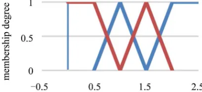
[image:7.595.207.541.88.319.2] [image:7.595.269.474.613.706.2]

In trying to illustrate and compare the methods as described above, a Monte-Carlo simulation study was perform to generate an (i.i.d) random samples, say y, according to IRD through the adoption of inverse transformation method with size n = 10, 30 and 90 to take care of small, medium and large data sets. The scale parameter λ = 0.3, 0.5, 1, 1.5, 2. Then, each observation of y was made Imprecision based on an appropriate selected membership function among four membership functions in the Imprecision Information System as the following

Figure 1.

The simulation program has been written by using MATLAB (R2010b) pro-gram. The results of Monte-Carlo simulation have been summarized in Table 1. The initial values required for proceeding modified Newton-Raphson method chosen to be the symmetrical rank regression estimators. The comparisons be-tween the parameter estimates were based on values from MSE where [8]:

(8)

[image:8.595.208.539.90.458.2]

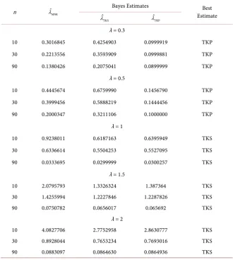
Table 1. MSE values for estimates of the scale parameter (λ) of IRD with different cases.

n λˆMNR

Bayes Estimates _Best Estimate

TKS

ˆ

λ λˆTKP

λ = 0.3

10 0.3016845 0.4254903 0.0999919 TKP 30 0.2213556 0.3593909 0.0999881 TKP 90 0.1380426 0.2075041 0.0899999 TKP

λ = 0.5

10 0.4445674 0.6759990 0.1456790 TKP 30 0.3999456 0.5888219 0.1444456 TKP 90 0.2000347 0.3211106 0.1000000 TKP

λ = 1

10 0.9238011 0.6187163 0.6395949 TKS 30 0.6336614 0.5504253 0.5527095 TKS 90 0.0333695 0.0299999 0.0300257 TKS

λ = 1.5

10 2.0795793 1.3326324 1.387364 TKS 30 1.4255994 1.2227846 1.2287826 TKS 90 0.0750782 0.0656017 0.065692 TKS

λ = 2

10 4.0827706 2.7752958 2.8630777 TKS 30 0.8928044 0.7653234 0.7693016 TKS 90 0.0883097 0.0864630 0.0864936 TKS

n: sample size; λˆMNR: maximum likelihood estimate of λ by newton-raphson; λˆTKS: Bayes estimate of λ of IRD based on square error loss function; λˆTKP: Bayes estimate of λ of IRD based on prec. loss function.

( )

_ˆ 1

(

ˆ

)

2

MSE

L j j

L λ λ

λ = −

=

∑

₍₃₀₎

ˆ

j

λ : is the estimate of λ_{respectively at the}_jth_run.

L: is the number of sample replicated chosen to be (500).

6. Conclusions and Recommendations

The most important conclusions of Monte-Carlo simulation results are:

Tierney and Kadane’s approximation based on square error loss function (TKS) estimate introduced the best perform compared with the different esti-mates for all sample sizes and for all cases except λ =0.3 and λ =0.5, where Bayes Estimate based on Precautionary loss function (TKP) is the best.

Based on this, we recommend,

(9)

DOI: 10.4236/ojapps.2019.98054 681 Open Journal of Applied Sciences 2) Using the TKP estimate to compute estimates of the scale parameter of IRD for all sample sizes and with the cases λ =0.3 and λ =0.5.

3) For further study, we suggest such type of work can be done by using other informative priors for the parameter of the IRD and also the parameter can be estimated by other methods.

4) Research can be applied to real data and demonstrate the importance of this distribution in practice.

Conflicts of Interest

The authors declare no conflicts of interest regarding the publication of this pa-per.

References

[1] Rao, G.S. and Mbwambo, S. (2019) Exponentiated Inverse Rayleigh Distribution and an Application to Coating Weights of Iron Sheets Data. Journal of Probability and Statistics, 2019, Article ID: 7519429.

https://doi.org/10.1155/2019/7519429

[2] Trayer, V.N. (1964) Doklady Acad, Nau, Belorus, U.S.S.R.

[3] Rasheed, H.A., Ismail, S.Z. and Jabir, A.G. (2015) Acomparison of the Classical Es-timators with the Bayes EsEs-timators of One Parameter Inverse Rayleigh Distribution,

International Journal of Advanced Research, 3, 738-749.

[4] Rasheed, H.A. and Aref, R.K.H. (2016) Bayesian Approach in Estimation of Scale Parameter of Inverse Rayleigh Distribution. Mathematics and Statistics Journal, 2, 8-13.

[5] Khoolenjani, N.B. and Shahsanaei, F. (2016) Estimating the Parameter of Exponen-tial Distribution under Type-II Censoring from Fuzzy Data. Journal of Statistical Theory and Applications, 15, 181-195. https://doi.org/10.2991/jsta.2016.15.2.8

[6] Norstrom, J.G. (1996) The Use of Precautionary Loss Function in Risk Analysis.

IEEE Transactions on Reliability, 45, 400-403. https://doi.org/10.1109/24.536992

[7] Tierney, L. and Kadane, J.B. (1986) Accurate Approximations for Posterior Mo-ments and Marginal Densities. Journal of the American Statistical Association, 81, 82-86. https://doi.org/10.1080/01621459.1986.10478240