A Review on Building Deterioration Prediction
using Statistical Analysis
Mayank Pachori1, Dr. Rajeev Kansal2
1
PG student, 2 Professor, Civil Engineering Department, Madhav Institute of Technology and Science, Gwalior, (M.P.) India
Abstract: Industrial surveys show that a very much sum of money is usually spent on repair and maintenance activities of the plants. This is more in case of deterioration, wear and corrosion. Therefore, by applying suitable and proactive approaches, the optimal maintenance time for the industrial structures can be determined and unnecessary maintenance costs can be reduced. Even a 5-10% reduction in maintenance costs will result in the industrial economy improvement. This paper emphasizes on the condition based preventive maintenance approach rather than the time based maintenance or corrective maintenance approaches because more accurate information regarding the building condition can be determined by using condition based approach. This paper shows the use of statistics to predict the deterioration of the building structures based on their current condition. Various types of statistical distributions are also illustrated. As the building deterioration is a non-negative phenomenon, it can best be analysed by the gamma distribution process which is a continuous type statistical distribution. Therefore, the gamma distribution is used as a tool in this paper for the deterioration prediction analysis.
Keywords: Industrial structures, maintenance, deterioration, statistics, gamma distribution.
I. INTRODUCTION
Various surveys carried out on industrial infrastructure reveal that a very much amount of money is consumed in the repair and maintenance activities of the industrial plants. This is due to lack of knowledge about the rate at which the deterioration or wear is taking place with time in any building structure. After certain period of operations, assets and their components start deteriorating with the age and cause failure of the whole system. . Determination of optimal maintenance decisions is widely recommended as an effective way of minimizing system failure and corresponding maintenance costs. Infrastructure maintenance practices are carried out by one of the two following methods:
A. Corrective maintenance approach
B. Preventive maintenance approach
Corrective maintenance approach includes the repairing or replacement of failed components and systems whereas in preventive maintenance approach the systematic inspection and correction of incipient failures is carried out before they develop into major defects. Preventive maintenance is planned maintenance of industrial structures and their components which is designed to improve structural life and avoid any unplanned maintenance activity. Recent years have seen increasing use of PM approaches with overall costs demonstrated to be lower than for a CM strategy. PM is widely used to mitigate asset deterioration and reduces the risk of unexpected failure and as a strategy can be sub-classified into two approaches; time-based maintenance (TBM), where maintenance activities take place at regular time intervals, and condition-based maintenance (CBM) where the maintenance of the structures takes place by information collected through condition sensing and monitoring processes (either manual or automated).
Preventive maintenance strategies (both time and condition based) are widely used for infrastructure life-cycle management decision making. These strategies can be planned and scheduled and their costs are typically lower than those for CM approaches. However early preventive maintenance intervention adds little to the reliability of the system and can lead to unnecessary costs, hence maintenance strategies often comprise a combination of preventive and corrective approaches.
Reasons for using preventive maintenance approaches in the current times:
1) Increasing the life expectancy of the structures.
2) Minimising the unexpected failure of the assets.
3) To determine the rate of deterioration for structures thereby applying condition based approaches.
4) To reduce the unnecessary maintenance costs which are higher while applying corrective maintenance strategies.
II. STATISTICS
Statistics and mathematics play vital role in the implementation of preventive maintenance strategies for industrial plants. Statistical distributions, particularly normal, gamma, Weibull, binomial and Poisson distributions, play important role in estimation during the quality control inspections and in predictive maintenance.
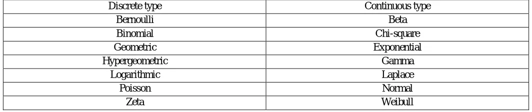
[image:2.612.40.572.182.294.2]Different types of statistical distributions are in use. They are categorised as discrete and continuous type. The following table I provides the list of various types of distributions.
Table I: List of Various Types of Statistical Distributions
Discrete type Continuous type
Bernoulli Beta
Binomial Chi-square
Geometric Exponential
Hypergeometric Gamma
Logarithmic Laplace
Poisson Normal
Zeta Weibull
A. Descriptive Statistical Terms
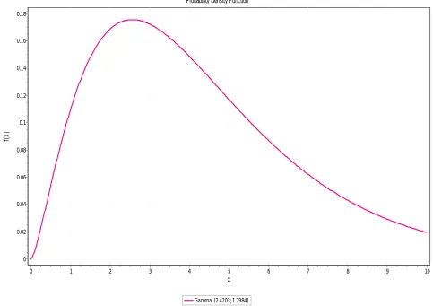
1) Probability Density Function (PDF): The PDF curve indicates regions of higher and lower probabilities for different values of random variables.
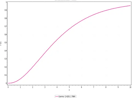
2) Cumulative Distribution Function (CDF): It is used to determine the probability that an observed value from the data set will be less than or equal to a certain value.
3) Inverse CDF: It is also known as quantile function which gives the value of the variable associated with a specific cumulative probability. Generally 95th percentile of the given probability is taken as quantile function.
4) Survival Function: The survival function or reliability function is the probability that a variable takes on a value greater than a certain value.
5) Hazard Function: It is also called the failure rate which is the ratio of probability density function (PDF) to the survival function. It is used in reliability applications to determine the instantaneous failure rate at any point in time.
Applications of various distributions: Weibull distribution can be used provide an estimate for life of parts which fail frequently like LEDs, electronic chips etc. Poisson distribution which is a discrete type distribution, can be used for events which are isolated. For example, no. of machinery breakdowns in a workshop can be illustrated by Poisson distribution. Gamma distribution can be applied to the areas where gradual degradation or change is occurring with the time.
III. METHODOLOGY
As the deterioration for any structure is a non-decreasing phenomenon which gradually increases with the time, the gamma process is considered to be an effective method to analyse and predict it. A gamma distribution is a non-negative continuous type statistical distribution with certain shape ( ) and scale or rate ( ) parameter values which can best be fit to the variable degradation data. The probability density function (PDF) for gamma distribution is given by
( ) =
( ) e > 0, > 0, > 0 (1)
Where gamma function, Γ(α) = ∫ (2) Let cumulative deterioration at time to are Z( ) Z( ), respectively. The deterioration increment from time to be independent of the cumulative deterioration at time and it is a non-negative quantity, i.e. Z( )− ( ) is independent of Z( ). Further, ( )− ( )~ (( )−( )) (3)
The gamma cumulative distribution function (CDF) of the damage is denoted as F(z)=∫ ( | , ) (4) Mean value of cumulative deterioration at time t is ( ) = αβ; Variance of cum. deterioration at time t is ( )=
Survival function is given by, S(z)= 1-F(z) (5)
Hazard rate gives the instantaneous failure rate and is given by H(z)= ( )
IV. DATA ANALYSIS AND RESULTS
The condition data of several industrial buildings is used in the analysis and deterioration prediction of buildings is carried out. Condition data: The elements are categorised into three groups according to the inspection data. Let the element condition in most recent inspection be Cc (recent condition) and the condition in previous inspection be Cp (previous condition). Then an element can be in one of the following three states S1, S2 or S3 which are mutually exclusive and exhaustive states defined based on two consecutive element conditions. The state are S1 , where Cc ≥ Cp ; S2 , where Cc < Cp and S3 , where Cc = Cp. S2 represents a state where the element has been renewed or refurbished as the current condition is improved compared to the previous condition.
S3 represents a state where the element has not been deteriorated as the condition remains the same.
S1 represents a state where the element has been actually deteriorated as the current condition is poor compared to the previous condition. The gamma process is used to model the incremental deterioration over time. Hence, the non-incremental datasets corresponds to states S2 and S3 are omitted in this study. The dataset corresponds to the state S1 that exhibits the positive increments are used in our gamma process.
Deterioration data: As the gamma process model is used for the damage or the deterioration, the inspection data are to be adjusted to derive the deterioration of the building element under consideration. Hence, the condition data are adjusted so that,
AccumulatedDeterioration = condition −1 (7)
For example, a brand new element which is in condition 1 has the accumulated deterioration 0 and a failed element which is in condition 10 has the accumulated deterioration 9. Hence, from this point onwards the paper refers to the deterioration rather than the condition of the element.
[image:3.612.64.547.357.698.2]Parameter estimation: With the help of a statistical distribution fit software, the parameter values and are calculated as it uses the maximum likelihood estimation method to derive out these factors automatically.
Fig. 1: Probability density function (PDF) curve for buildings
Probability Density Function
Gamma (2.4203; 1.7984) x
10 9
8 7
6 5
4 3
2 1
0
f(
x
)
0.18
0.16
0.14
0.12
0.1
0.08
0.06
0.04
0.02
Fig. 2: Cumulative distribution function (CDF) curve
Fig.3: Survival function curve Cumulative Distribution Function
Gamma (2.4203; 1.7984) x
10 9
8 7
6 5
4 3
2 1
0
F
(x
)
1
0.9
0.8
0.7
0.6
0.5
0.4
0.3
0.2
0.1
0
Survival Function
Gam ma (2.4203; 1.7984)
x
10 9
8 7
6 5
4 3
2 1
0
S
(x
)
1
0.9
0.8
0.7
0.6
0.5
0.4
0.3
0.2
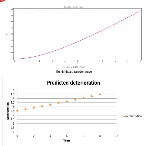
Fig. 4: Hazard function curve
Fig. 5: Predicted deterioration curve for building structures based on the inspection data
V. CONCLUSIONS
Reliability based approaches of deterioration prediction for infrastructure assets have been reviewed and gamma process has been selected as a possible mechanism to be examined. From the above concluded analysis the following results can be inferred:
A. The expected deterioration rating for the Year 0 (2016) is calculated as 2.54 which signifies the current condition rating for the Year 0 as 3.54 i.e. somewhere between condition 3 & 4. According to condition rating table it corresponds to an asset which is in very good overall condition with deterioration and serviceability loss small in nature.
B. To keep the infrastructure assets in condition nearby 4 or better it is suggested to apply the inspection and maintenance procedures by Year 3.
C. Estimated shape ( ) parameter value is 2.4203 and rate ( ) parameter value is 1.7984.
D. The expected life of the industrial buildings based on the above analysis is calculated as 56 years.
E. According to the inverse CDF value based on this inspection data analysis, 95% portion of the industrial buildings will fail when the deterioration rating reaches 9.73 (condition rating >10).
Cumulative Hazard Function
Gamma (2.4203; 1.7984) x
10 9
8 7
6 5
4 3
2 1
0
H
(x
)
3.2
2.8
2.4
2
1.6
1.2
0.8
0.4
0
0 0.5 1 1.5 2 2.5 3 3.5 4 4.5 5
0 2 4 6 8 10 12
D
e
te
ri
o
ra
ti
o
n
Years
Predicted deterioration
REFERENCES
[1] Edirisinghe R., Setunge S., Zhang G. (2013),”Application of gamma process for building deterioration prediction”. Journal of Performance of Constructed Facilities, Vol. 27, No. 6, December 2013. ©ASCE, ISSN 0887-3828/2013/6-763-773
[2] Daneshkhah A., Stocks N.G., Jeffrey P., (2017).”Probabilistic sensitivity analysis of optimized preventive maintenance strategies for deteriorating infrastructure assets”. Reliability engineering and system safety. 163(2017),33-45
[3] vanNoortwijk, J.M. (2009).“A survey of the application of gamma processes in maintenance.” Reliab. Eng. Syst. Saf., 94(1), 2-21. [4] Cinlar E., Bazant Z.P., Osman E. (1977). “Stochastic process for extrapolating concrete creep.” J. Eng. Mech. Div., 103(1), 1069-1088.
[5] Lawless J., Crowder M. (2004).”Covariates and random effects in a gamma process model with application to degradation and failure”. Lifetime Data Anal., 10(3), 213-227.
[6] K. Venkataraman, Maintenance engineering and management; 2007
[7] NPTEL, “Analytic continuation and the gamma function”. Module-04, Lecture-09; IIT Madras.
[8] Kleiner, Y. and B. Rajani, Comprehensive Review of Structural Deterioration of Water Mains: Statistical Models. Urban Water Journal, 2001. 3: p. 131-150. [9] Lou, Z., et al., Application of Neural Network Model to Forecast Short-Term Pavement Crack Condition: Florida Case Study. Journal of Infrastructure
Systems, ASCE, 2001. 7(4): p. 166-171.
[10] Wirahadikusumah, R., M.D. Abraham, and T. Iseley, Challenging Issues in Modeling Deterioration of Combined Sewers. Journal of Infrastructure Systems, ASCE, 2001. 7(2): p. 77-84.