Munich Personal RePEc Archive
High-dimensional macroeconomic
forecasting using message passing
algorithms
Korobilis, Dimitris
University of Glasgow
15 September 2019
Online at
https://mpra.ub.uni-muenchen.de/96079/
High-dimensional macroeconomic forecasting using
message passing algorithms
✯
Dimitris Korobilis
❸University of Glasgow
Abstract
This paper proposes two distinct contributions to econometric analysis of large information sets and structural instabilities. First, it treats a regression model with time-varying coefficients, stochastic volatility and exogenous predictors, as an equivalent high-dimensional static regression problem with thousands of covariates. Inference in this specification proceeds using Bayesian hierarchical priors that shrink the high-dimensional vector of coefficients either towards zero or time-invariance. Second, it introduces the frameworks of factor graphs and message passing as a means of designing efficient Bayesian estimation algorithms. In particular, a Generalized Approximate Message Passing (GAMP) algorithm is derived that has low algorithmic complexity and is trivially parallelizable. The result is a comprehensive methodology that can be used to estimate time-varying parameter regressions with arbitrarily large number of exogenous predictors. In a forecasting exercise for U.S. price inflation this methodology is shown to work very well.
Keywords: high-dimensional inference; factor graph; Belief Propagation; Bayesian shrinkage; time-varying parameter model
JEL Classification: C11, C22, C52, C55, C61
✯This paper has significantly improved based on suggestions from two anonymous referees, an Associate Editor, and the Editor (Todd Clark), whom I gratefully acknowledge. I would like to thank Fabio Canova, Eric Ghysels, George Kapetanios, Gary Koop, Massimiliano Marcellino, Geert Mesters, Davide Pettenuzzo, Giorgio Primiceri, Giuseppe Ragusa, Giovanni Ricco, Lucrezia Reichlin, Frank Schorfheide, Herman van Dijk, Hal Varian and Mike West for useful comments and/or stimulating discussions. I would also like to thank Joshua Chan, and Maria Kalli/Jim Griffin for sharing MATLAB codes that replicate time-varying parameter specifications suggested by these authors. Additionally, I would like to acknowledge helpful comments and questions from participants at the 2017 Deutsche Bundesbank Forecasting Workshop; the 2017 Norges Bank conference on “Big data, Machine Learning and the Macroeconomy”; the 10th ECB Workshop on Forecasting Techniques: “Economic Forecasting with Large Datasets”; the BayesComp / ISBA 2018 conference; the 3rd annual Now-Casting.com Workskhop; the 2018 Budapest School for Central Bank Studies; the 2019 Econometric Institute workshop “Machine Learning Meets Econometrics”; and the 2019 Joint Research Centre European Commission workshop “Big Data and Economic Forecasting”. Finally, I would like to acknowledge useful feedback from seminar participants at various Universities and central banks.
1
Introduction
As a response to the increasing linkages between the macroeconomy and the financial
sector, as well as the expanding interconnectedness of the global economy, empirical
macroeconomic models have increased both in complexity and size. For that reason,
estimation of modern models that inform macroeconomic decisions – such as linear
and nonlinear versions of dynamic stochastic general equilibrium (DSGE) and vector
autoregressive (VAR) models – many times relies on Bayesian inference via powerful
Markov chain Monte Carlo (MCMC) methods.1 However, existing posterior simulation
algorithms cannot scale up to very high-dimensions due to the computational inefficiency
and the larger numerical error associated with repeated sampling via Monte Carlo; see
Angelino et al. (2016) for a thorough review of such computational issues from a machine
learning and high-dimensional data perspective. In that respect, while Bayesian inference is
a natural probabilistic framework for learning about parameters by utilizing all information
in the data likelihood and prior, computational restrictions might make it less suitable for
supporting real-time decision-making in very high dimensions.
This paper introduces to the econometric literature the framework of factor graphs
(Kschischang et al., 2001) for the purpose of designing computationally efficient, and easy
to maintain, Bayesian estimation algorithms. The focus is not only on “faster” posterior
inference broadly interpreted, but on designing algorithms that have such low complexity
that are future-proof and can be used in high-dimensional econometric problems with
possibly thousands or millions of coefficients. While a graph, in general, is a structure
that allows the representation of objects that are related in some sense2, a factor graph
representation of a high-dimensional vector of model parameters, in particular, depicts how
1See Herbst and Schorfheide (2015) and Koop and Korobilis (2010) for detailed discussion of Bayesian
computation in DSGE and VAR models, respectively.
2The most popular use of graphs in economics is to represent networks of agents, banks, social networks
each of its scalar elements is connected with each other based on the functional form of their
joint posterior distribution. As a result, the factor graph representation provides a visual
tool for the decomposition of a high-dimensional joint posterior distribution into smaller,
tractable parts. By doing so, factor graphs can be used to design parallel versions of MCMC
algorithms, as well as efficient iterative algorithms calledmessage passing algorithms – the
latter being the concept of interest in this paper.3
Having the factor graph as the starting point, interest lies in an estimation strategy
called the sum-product algorithm which is not well known in mainstream statistics, despite
the fact that it is computationally powerful (Wand, 2017, p. 137-138). The sum-product
algorithm is a general rule in factor graphs that allows to iteratively approximate marginal
(posterior) distributions. When applied to a parametric problem with arbitrary likelihood
and prior functions, the so-called Generalized Approximate Message Passing (GAMP)
algorithm introduces further Gaussian and quadratic approximations to the possibly
complicated expressions derived by the sum-product iterative algorithm. Proposed
by Rangan (2011), GAMP is an extension of the popular Approximate Message
Passing (AMP) algorithm of Donoho et al. (2009). The GAMP algorithm has
desirable properties, namely, high-dimensional scalability, parallelizability, and effortless
maintenance. Therefore, the first task of this paper is to analyze the concept of message
passing algorithms in general; simplify the jargon stemming from signal processing,
computing science, and similar literatures that have introduced such algorithms; and show
how GAMP, in particular, can lead to efficient posterior inference in very high-dimensions.
At the same time, a second important task is to provide compelling evidence that the
proposed algorithm is relevant for modeling macroeconomic variables. For that reason, I
3Message passing algorithms are dynamic programming methods designed for efficiently performing
utilize a regression model setting with time-varying coefficients, stochastic volatility, and
exogenous predictors. Regression models featuring time-varying parameters (TVPs) have
been popular in economics at least since the seminal work of Cooley and Prescott (1976).
More recently, there has been a systematic effort to introduce efficient MCMC algorithms
for flexible estimation and shrinkage in Bayesian TVP models; see Belmonte et al. (2014),
Chan et al. (2012), Giordani and Kohn (2008), Groen et al. (2013), Kalli and Griffin
(2014), Koop and Potter (2007), Kowal et al. (2018), Nakajima and West (2013), Roˇckov´a
and McAlinn (2018) and Stock and Watson (2007) among others. These are examples of
carefully designed MCMC algorithms that result in flexible joint modeling of structural
instabilities and parameter shrinkage, but that may not be scalable to very high dimensions
due to their reliance on repeated sampling via Monte Carlo.
As a consequence, a novel empirical contribution introduced in this paper is to estimate
a time-varying parameter regression model by using an observationally equivalent
high-dimensional static regression form, and to address computational concerns by using
message passing inference. With T observations and p predictors, the TVP model can
be written as a static regression with the same T observations but (T + 1)p covariates –
where the product (T + 1)p can easily be in the order of tens of thousands in standard
macroeconomic applications. This static representation of the time-varying parameter
model is anything but new, however, its estimation in the past has been exclusively
tackled by specifying an additional hierarchical random walk (or some times stationary
autoregressive) model for all time-varying parameters. This hierarchical form allows
for inference using state-space methods and at the same time it can be interpreted as
an informative shrinkage prior that makes estimation of this high-dimensional problem
feasible. Instead I propose to completely drop this “random-walk prior” and the resulting
state-space representation, and estimate the time-varying parameter model as a
shrinkage prior inspired by Tipping (2001). That way, by casting the TVP regression
model into equivalent static form, standard shrinkage principles can be used in order to
determine by how much coefficients evolve over time, or whether their value is zero and
they are completely irrelevant. Most importantly, the use of the low-complexity GAMP
algorithm ensures that the static form of the TVP regression with (T + 1)pcovariates can
be estimated quickly. The benefits of this algorithm and modeling strategy are illustrated
using a forecasting exercise for monthly U.S. inflation that extends Stock and Watson
(1999) to the TVP setting. The static form of the TVP regression estimated with GAMP
is contrasted with powerful but slow MCMC algorithms for TVP models, such as Chan
et al. (2012) and Kalli and Griffin (2014). The proposed approach, by incorporating a
larger number of predictors and by shrinking coefficients flexibly, does perform significantly
better compared to competitors in out-of-sample forecasting.
In the next section I introduce the general framework of factor graphs on random
variables (parameters) and with the help of a toy example I show how this framework
allows for efficient calculation of marginal distributions. Next, in Section 3 I introduce
the TVP regression setting, rewrite the likelihood in static regression form and specify a
shrinkage “sparse Bayesian learning” (SBL) prior. Under the given functional forms for the
likelihood and prior, I proceed to derive a GAMP algorithm for this particular problem. In
Section 4 the benefits of the proposed high-dimensional modeling approach are evaluated
in a forecasting exercise for U.S. price inflation. Section 5 concludes the paper.
2
Factor graphs and the sum-product algorithm
A factor graph represents the way a global function of several variables can be decomposed
into a product of simpler functions (“factors”). Consider a generic example with discrete
as
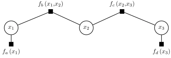
p(x1, x2, x3) =fa(x1)fb(x1, x2)fc(x2, x3)fd(x3), (1)
wherefa, fb, fc, fdare the factors that have known functional forms.4 This simple example
can be depicted using the factor graph of Figure 1, where circles denote the place of random
variables in the graph and filled boxes denote the factors/functions.5
fb(x1,x2) fc(x2,x3)
x1 x2 x3
[image:7.612.167.447.231.326.2]fa(x1) fd(x3)
Figure 1: Simple factor graph representation of the decomposition of joint function
p(x1, x2, x3).
Consider now calculation of the marginal distribution of xi. This is a computationally
demanding task due to the fact that it involves integration (summation, in the discrete
variable case) over all variables other than xi
p(xi) = X
x\xi
p(x1, x2, x3), (2)
wherex\xi denotes the setxwith the elementxi removed. As an example, if the variables
in x have two states (e.g. they are binary variables), then the above sum would only
require 23 operations. However, for high number of states and/or variables computational
requirements proliferate substantially. Nevertheless, if p(x1, x2, x3) is replaced with the
4In the next section, the discrete random variables x are replaced by continuous model parameters,
and the factors/functions are conditional or marginal probability distributions over these parameters.
5In graph theory, symbols like the boxes and the circles in this example are called nodes or vertices.
expression in (1) it can be seen that not each variable is coupled to every other one, and
this feature can be exploited in order to simplify the summation. For example, in the case
of variable x1, Figure 1 depicts that it is directly connected to x2 and the factors fa(x1)
and fd(x1, x2), but it is only indirectly connected to x3 and the remaining factors. Put
differently, we can simplify (2) via identity (1) as follows
p(x1) = X
x2 X
x3
fa(x1)fb(x1, x2)fc(x2, x3)fd(x3) (3)
= fa(x1) X
x2
fb(x1, x2) X
x3
fc(x2, x3)fd(x3). (4)
The second line of the equation above implies less algorithmic operations compared to the
expression in the first line.
It should be clear at this point that the role of the factor graph representation is to
allow to pin down the full path of influence that each variablexi exerts on other variables.
As a consequence, by having this path of influence, only the required factors fj can be
used when calculating marginal distributions, which increases computational efficiency.
This is where the concept of message passing formalizes such an efficient procedure for
computing marginals. Each variable node passes messages to the next variable, where
these messages are real-valued functions showing the influence that this variable exerts on
all other variables. In the remainder of this Section message passing inference is introduced
and the sum-product algorithm is derived, such that simplifications similar to the ones in
equations (3)-(4) are formalized mathematically. Subsequently, in Section 3 the results of
this toy example with three discrete random variables (parameters) can be generalized to
a high-dimensional regression setting with possibly millions of parameters. More detailed
introductions to these concepts can be found in popular machine learning textbooks, such
as Barber (2012) and Bishop (2006). A recent introduction of message passing inference
Denote withµxi→fj the message sent from variablexito functionfj, and withµfj→xithe
message sent from factor node fj to variable node xi, wherei= 1,2,3 and j =a, b, c, d in
our simple example with three variables and four factors. The message sent from variable
xi to factor nodefj is equal to the product of all messages arriving to nodexi except from
the message coming from the target node fj:
µxi→fj =
Y
k∈N(xi),k6=j
µfk→xi, (5)
where N(xi) is the set of neighboring (factor) nodes to xi. Similarly, the message sent
from factor node fj to variable node xi is given by the sum over the product of the factor
function fj itself and all the incoming messages, except the messages from the target
variable node xi:
µfj→xi =
X
x\xi
fj(x) Y
l∈N(xi),l6=i
µxl→fj. (6)
Due to the form of the equation above, algorithms that are designed to iterate between (5)
and (6) are calledsum-product algorithms; see also respective equations for the regression
model in the next section.
In the special case where xi is an external node (as is the case with x1 and x3 in this
example) it holds thatµxi→fj = 1. Similarly, iffj is an external factor node (seefa(x1) and
fd(x3) in Figure 1) it holds thatµfj→xi =fj(xi). Equations (5)-(6) define the iterations of
the so-called sum-product algorithm (also called Belief Propagation; see Pearl, 1982), that
the Bayesian networks literature). Upon convergence, it can be shown6 that
p(xi)∝ Y
m∈N(xi)
µfm→xi, (7)
that is, the marginal distribution of variable xi is simply the product of all messages
received only from factor nodes that are connected to xi.
Consider for example calculation of p(x2). Starting from the left of the graph, the
messages emitted to node x2 are:
µfa→x1 = fa(x1), (8)
µx1→fb = µfa→x1 =fa(x1), (9)
µfb→x2 = X
x1
fb(x1x2)µx1→fb, (10)
where the first identity holds becausefa(x1) is an external factor node, the second identity
is a result of equation (5), and the third identity is a result of (6). Similarly, the messages
that arrive to x2 stating from the right of the graph are
µfd,x3 = fd(x3), (11)
µx3→fc = µfc→x3 =fd(x3), (12)
µfc→x2 =
X
x3
fc(x2, x3)µx3→fc, (13)
where again the first identity results from the fact that fd(x3, x4) is an external factor
node, the second results from equation (5) and the third from equation (6). Therefore, the
6It is beyond the scope of this paper to derive and prove the algorithm, and the reader is referred to
marginal distribution of x2 is now
p(x2)∝µfb→x2 ×µfc→x2. (14)
Using similar arguments we can derive p(x1) and p(x3).
In this particular example, the formula derived in (14) might seem redundant as for
a wide class of distributions p(•), one can simply calculate the marginal distribution
of x2 using numerical integration. However, in high dimensions with many random
variables, the sum-product rule can provide us with scalable and parallel posterior inference
algorithms that can be several times faster compared to conventional algorithms that
iterate sequentially (e.g. Gibbs sampler). It can be shown that the sum-product (Belief
Propagation) algorithm is a special case of the more general expectation propagation
algorithms that have been very popular in Bayesian machine learning; see Vehtari et al.
(2018). Finally, note at this point that there is no mention about how to approximate
the summations in (6), which will not necessarily be tractable. Given the sum-product
formula, there are several algorithms that would allow for the approximation of the required
messages which are functions of the factorsfj. For example, Wand (2017) develops message
passing inference inspired by the variational Bayes method. In the next section I adopt a
recently developed algorithm (Generalized Approximate Message Passing) that performs
3
Econometric Methodology
3.1
Time-varying parameter regression
The starting point is the following time-varying parameter (TVP) regression with
stochastic volatility of the form
yt =xtβt+εt, (15)
subject to an initial condition forβtatt = 0 (denoted asβ0), whereytis thetthobservation
on the variable of interest,t= 1, ..., T,xtis a 1×pvector of predictors (possibly including
lags of yt), βt is a p×1 vector of coefficients, and εt∼N(0, σt2) withσt2 the time-varying
variance parameter. It is desirable to estimate the initial condition in this model, rather
than assume it is knonw. For that reason, following Fr¨uhwirth-Schnatter and Wagner
(2010), this model can be written using an equivalent non-centered parametrization that
allows to split the parameter βt into a part that is constant (which is equivalent to its
initial condition β0), and an “add-on” time-varying part with initial condition fixed to
zero. The equivalent specification is
yt =xtβe+xtβet+εt, (16)
where now βet has initial condition zero and it holds that βt = βe+βet. As shown in
Belmonte et al. (2014) this parametrization allows to use shrinkage priors to determine
whether a variable has constant coefficient (by only shrinking the time-varying part), or it
is completely irrelevant for modeling y (by shrinking both the constant and time-varying
parts to zero). More details of this approach are provided in the Online Appendix, Section
The TVP regression can be written in the following equivalent static regression form
y=Xβ+ε, (17)
where y = [y1, ..., yT]′ and ε = [ε1, ..., εT]′ are column vectors stacking the observations yt
and εt respectively, β = h
e
β′,βe′ 1, ...,βeT′
i′
is a (T + 1)p×1 vector, and
X=
x1 x1 01×p ... 01×p 01×p
x2 01×p x2 ... 01×p 01×p
... ... . .. ... ... ...
xT−1 01×p 01×p ... xT−1 01×p
xT 01×p 01×p ... 01×p xT , (18)
is a T ×(T + 1)p matrix. It is evident that the first p columns of X specify a constant
parameter regression and its remaining columns add “time-dummies” to that regression.
The Gram matrix (X′X) is of rankT and theq= (T+1)p, in total, regression coefficients in
(17) cannot be estimated with OLS. For that reason, following a long-standing tradition
in engineering, economists tend to assume that βt (similarly for βet in the non-centered
parametrization) typically follows a random walk of the form βt = βt−1 + ηt, where
ηt ∼ N(0, Q) for some p× p symmetric, positive-definite covariance matrix Q. This
random walk regression for βt allows to write the full time-varying parameter regression
model in familiar state-space form, and also provides the additional information needed
to estimate βt using data y and X. By doing so, estimation typically relies on Markov
chain Monte Carlo methods by means of a simulation smoother; see Primiceri (2005) for
a representative example. From a Bayesian point of view this additional information can
be viewed as a conditional hierarchical prior of the form p(βt|βt−1) ∼ N(βt−1, Q) that
as an ill-posed problem where OLS does not have a unique solution and regularization is
imperative for estimation.
In this paper I adopt this shrinkage view of the time-varying parameter regression
model and propose an alternative inference strategy. That is, inference is done without
reference to the useful but rather informative and subjective conditional hierarchical prior
for βt given βt−1 outlined above. Instead, the time-varying parameters are recovered
by estimating directly equation (17) using data-based hierarchical shrinkage priors. In
particular, I follow Tipping (2001) and define the following independent hierarchical prior
for each element βi of the vector β, i= 1,2, ...,(T + 1)p,
p(βi|αi) = N 0, αi−1
, (19)
p(αi) = Gamma(a, b). (20)
This conditionally Normal prior for βi and Gamma prior for the precision parameter αi
is a scale mixture of Normal representation of a Student-t prior. Tipping (2001) calls
this heavy-tailed prior a sparse Bayesian learning (SBL) prior, and I adopt this name
henceforth; see also Korobilis (2013) for a detailed explanation why such hierarchical
priors have good shrinkage properties. I follow Tipping (2001) and present all empirical
results using the uniform hyperpriors (over a logarithmic scale) a=b = 1×10⁻¹⁰.
Two additional comments are in order regarding this time-varying parameter
regression. First, the number of columns of X is q = (T + 1)p, therefore, the number
of coefficients grows rapidly. For example, with 700 monthly observations and only 100
predictors, we end up with 70,100 regression coefficients. As a consequence, it is imperative
to choose a fast estimation algorithm that approximates the parameter posterior, and this
is where the scalability of message passing algorithms comes into play. Second, there is
no mention yet of inference on σ2
GAMP inference algorithm is outlined. In a nutshell, estimation of stochastic volatility
σ2
t also follows the same shrinkage principles defined for βt. That is, it is shown that we
can write estimation of σ2
t as a high-dimensional regression problem, without having to
assume any kind of first-order Markov dependence to σ2 t−1.
3.2
A factor graph representation of Bayesian regression
At this point we have all the necessary ingredients in order to cast the static form of the
time-varying parameter regression in equation (17) into a factor graph form.7 Consider
first an independent (but not necessarily i.i.d) prior for β, denoted p(β) = Qqi=1p(βi),
and the resulting posterior from Bayes Theorem
p(β|y) ∝ p(y|β)p(β) (21)
=
T Y
t=1
p(yt|β) q Y
i=1
p(βi). (22)
The exact marginal posterior of βi, i= 1, ..., q is of the form
p(βi|y) = Z
p(β|y)dβj6=i, (23)
∝ Z
p(y|β)p(β)dβj6=i, (24)
= p(βi) Z
p(y|β)
q Y
j=1,j6=i
p(βj)dβj6=i, (25)
where dβj6=i denotes integration over the whole set of q − 1 parameters βj for j 6= i.
Therefore, the formula above requires integration over a (q−1)-dimensional integral, a
numerical problem that can become computationally infeasible for a high-dimensional
7For the sake of brevity, notation for prior, posterior and likelihood distributions is generic, that is,
vector β.
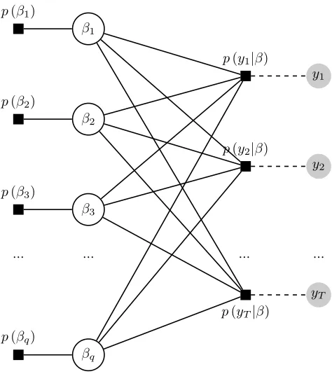
We can now call the framework of factor graphs in order to factorize efficiently the
marginal posteriors of β. The factor graph representation of the regression model is
depicted in Figure 2. Based on this figure, the marginal posterior of βi, presented in
equation (25), can be defined as the product of incoming messages at nodeβi in the graph
p(βi|y) = µp(βi)→βi
T Y
t=1
µp(yt|β)→βi. (26)
Similar to equation (8) in the example of Section 2, the message µp(βi)→βi is an external
factor node and for that reason it is equal to the prior p(βi). Generalizing the example
sum-product rule derived in equations (5) - (6) of the previous section, we can write the
messages from p(yt|β) ∀t to βi using the following expression
µp(yt|β)→βi =
Z
p(yt|β) p Y
j=1,j6=i
µβj→p(yt|β)dβj6=i. (27)
In the decomposition above, the message from node βj to function (factor)p(yt|β) is the
product of all incoming messages to node βi, excluding the message coming from p(yt|β)
itself
µβj→p(yt|β)=p(βj)
T Y
s=1,s6=t
µp(ys|β)→βj. (28)
We can see in equations (27)-(28) that in order to obtain the messageµp(yt|β)→βiwe need
p(β1)
β1
p(y1|β)
y1
p(β2)
β2
p(y2|β)
y2
p(β3)
β3
... ... ... ...
p(yT|β)
yT
p(βq)
[image:17.612.180.417.93.360.2]βq
Figure 2: Factor graph representation for the high-dimensional regression model.
using the following iterative sum-product scheme
µ(pr(+1)yt|β)→β
i =
Z
p(yt|β) q Y
j=1,j6=i
µ(βr)
j→p(yt|β)dβj6=i, (29)
µ(βrj+1)→p(yt|β) = p(βj) T Y
s=1,s6=t
µ(pr()ys|β)→βj, (30)
where the superscript (r) denotes the rth iteration of the algorithm. In graphs with a
tree structure, one iteration of the algorithm above will always recover the exact marginal
posteriors for the parameters βi. In a factor graph with loops there are no guarantees that
the sum-product rule will converge to a good fixed point. However, the sum-product rule
can still achieve a good approximation and this is the reason why it is used extensively in
applications of coding theory, machine vision, and compressive sensing that have a loopy
jargon for the static regression in equation (17), algorithmic convergence is achieved if the
correlation of right-hand side predictors is not excessively high. If this is not the case,
the joint posterior of the coefficients β might also be highly correlated, which would make
inference solely based on the marginal posteriors p(βi) less accurate. In our benchmark
time-varying parameter regression in (17), correlation is by default not excessively high due
to the fact that the Gram matrixX′Xhas a certain block-diagonal structure that allows for
a general sparse correlation pattern – even if within a given block correlation may be high.
In the empirical application, predictor variables are mainly principal components or lags
thereof, such that correlation within each block is also low. Finally, note that the specific
time-decomposition of the likelihood function does not accommodate autoregressive and
general time-series models, where the likelihood at time t may be written conditional on
past observations. In the empirical application it is found that, despite this approximation,
autoregressive coefficients are recovered accurately.8
3.3
Generalized Approximate Message Passing
While the core of any message passing algorithm is fully described by the sum-product
iterations, deriving the exact functional form of the messages in equations (29) and
(30) under the regression likelihood and the Student-t hierarchical prior implies that
cumbersome integrations might be necessary. The GAMP algorithm introduces certain
Gaussian approximations to the sum-product iterations. Unlike Laplace approximations,
that is, Gaussian approximations to parameter posteriors that many times can be poor,
the GAMP approximation is fully based on asymptotic results that make it more reliable
8A simulation exercise in the Online Appendix, Section C.3, generating artificial data from an AR(4)
model, also verifies that the proposed GAMP algorithm performs well even if the likelihood function is not
i.i.d. Another important assumption that affects performance of GAMP is thatXis mean-zero Gaussian;
as the number of predictors grows large. First, when q → ∞ a central limit theorem
(CLT) postulates that the messagesQqj=1,j6=iµβj→p(yt|β)can be approximated by a Gaussian
distribution with respect to the uniform norm.9 This result means that messages in (27)
can be represented to be proportional to a Gaussian distribution. A second approximation
involves taking the Taylor-series expansion of terms in the messages, so that the first two
moments (mean and variance) ofp(βi|y) can be obtained analytically up to the omission of
O(1/q) terms. Exact derivation of these approximations involves many tedious steps and
transformations, and the reader is referred to the Online Appendix for more details. What
is important to stress at this point is that both the CLT and Taylor-series approximations
vanish as q→ ∞with q/T →δ for some constantδ; see Rangan (2011) and Rangan et al.
(2016) for more details. This is an example of the “blessing of Big Data” – rather than
the “curse of dimensionality” embedded in many traditional estimation algorithms – as
the GAMP algorithm fully facilitates the large q asymptotics.
Deriving the GAMP algorithm involves several steps and lengthy proofs which are
left for the Online Appendix. The final product of all the approximations to the two
sum-product update equations (29) - (30), is a simple iterative algorithm that provides
an approximation to the mean and variance of p(βi|y). The algorithm iterates through
computationally trivial scalar multiplications and additions that result in worst case
algorithmic complexity of O(T q). That is, estimation of the marginal parameter posterior
distribution does not involve costly operations such as high-dimensional integration or
inversion of large matrices. This feature implies that the algorithm can handle regressions
with an excessively large number of predictors with the same ease it can handle smaller
9This is a result of the Berry-Esseen central limit theorem which states that a sum of random variables
regression models. Convergence is achieved when the difference between estimates of the
posterior mean of β between two consecutive iterations is below a pre-specified tolerance
level. Other parameters can be updated by combining the GAMP algorithm with EM
updates.10 This feature is explained in the Online Appendix, where it is shown how to
update the hyperparameter αi introduced in the hierarchical prior of equation (20).
A sketch of the algorithm is provided in Algorithm 1. This is a simplified version
that focuses on estimation of β by assuming that the regression variance and prior
hyperparameters are all known and fixed. Following the analysis in Section 2, the algorithm
can be split into two steps: i) evaluating all messages that leave each variable node βj
(output), and ii) evaluating all messages that arrive at each variable node βj (input). The
final product is estimates of the posterior mean and variance of βj which are denoted as
b
βi and bτiβ, respectively. At the core of the calculation of the posterior mean and variance
are the scalar functions gin and gout. Derivation of the exact form of these two functions
depends on the form of the prior distribution and the likelihood. Online Appendix, Section
B, provides a detailed algorithm in the case of the regression likelihood in equation (17)
and the prior in (19)-(20). In any case, Rangan (2011) shows that regardless of the form
of the nonlinear scalar functions gin and gout, the worst-case complexity of the GAMP
algorithm is not affected and is always O(T q).
10See Al-Shoukairi et al. (2018) and Zou et al. (2016) for examples of how to derive EM updates for
Algorithm 1 Generalized Approximate Message Passsing (GAMP) with known variance and prior hyperparameters
1: Initialize βbi(0) = 0 and bτ β,(0)
i = 100∀i= 1, ..., q, and set bs (0)
t = 0 ∀t = 1, ..., T.
2: r= 1
3: while kβb(r)−βb(r−1)k →0 do
4: 1) Output Messages Step:
5: for t= 1 to T do
6: bc(tr) =
Pq
i=1Xt,iβb (r−1)
i −bs
(r−1)
t bτ
c,(r) t
7: bτtc,(r)=
Pq
i=1X2t,ibτ β,(r−1) i
8: bs(tr) =gout
b
c(tr),bτ c,(r) t , yt
9: bτts,(r) =−∂∂bcgout
bc(tr),bτ
c,(r) t , yt
10: end for
11: 2) Input Messages Step:
12: for i= 1 to q do
13: db(ir) =βbi(r−1)+τbid,(r)PTt=1Xt,ibs(tr)
14: bτid,(r)=PTt=1X2t,ibτts,(r)−1
15: βbi(r)=gin
b
d(ir),bτid,(r)
16: bτiβ,(r)=bτ
d,(r) i ∂∂dbgin
b
d(ir),bτ d,(r) i
17: end for
18: r =r+ 1
19: end while
20: Obtain mean and variance of β asβb=βb1(r), ...,βb (r) q
and τβ =τbβ,(r) 1 , ...,τb
β,(r) q
The algorithm above assumes a known regression variance, e.g. normalized to be one.
Of empirical interest is the derivation of an update rule for the variance parameter when
this is both unknown and time varying. Here I propose a novel, computationally trivial
estimator of the variance that builds on approximations used in the Bayesian stochastic
volatility estimator of Kim et al. (1998). First, we write the regression model in (17) in
the following form
y =Xβ+ Σv, (31)
where Σ is a T ×T diagonal matrix with the time-varying standard deviations σt on its
can re-write the above model as
logy−Xβb2
= log diag(Σ)2+ log(v2),⇒ (32)
e
y = σe2+ev, (33)
where diag(Σ)2 is a T ×1 vector with elements σ2
t ∀t ∈ [1, T], and variables with a e•
denote quantities in log-squares. In particular, the distribution of ev is log−χ2 with one
degree of freedom. Following Kim et al. (1998) we can approximate this with a mixture of
seven Normal distributions with means µi, variancesVi and component weights πi, where
i= 1, ...,7 and Piπi = 1.11 Then equation (33) can be replaced with the following set of
seven equations
e
y=σe2+ui, i= 1, ...,7, (34)
where ui ∼ N(µi, Vi). An estimator of the T ×1 vector of log-volatilities is of the form
Ei(eσ2) =ye−µi, and the final volatility estimate at time t is
b
σt2 = exp 7 X
i=1
πi(yet−µi)/7 !
. (35)
Similar expressions can also be derived for the posterior variance of σ2
t if desired, for
example, when computing the posterior predictive density via simulation. It turns out that
the resulting estimate of volatility is similar to the standard stochastic volatility estimator
of Kim et al. (1998), but it is much less persistent due to the lack of dependence of σ2 t
on σ2
t−1. More evidence on the excellent properties of this simple estimator of stochastic
volatility is provided in the Online Appendix, Section D.1.
Finally, Online Appendix, Section C, provides detailed Monte Carlo evidence on the
11The exact values of µ
usefulness of the proposed econometric specification and algorithm. By simulating artificial
data from models with various patterns of time-variation in parameters, it is assessed how
good the specification in equation (17), with the assistance of the sparse Bayesian learning
prior, is at recovering the true time-varying parameters. At the same time, a second
simulation exercise shows the ability of the GAMP algorithm with shrinkage prior to
perform high-dimensional shrinkage even in cases with more predictors than observations.
A final simulation exercise discusses the stability of the GAMP algorithm in models with
correlated predictors, and assesses numerically the case where the likelihood function is not
i.i.d. While the results of the simulated data exercises suggest that the proposed algorithm
provides a reasonable balance between computational speed and estimation accuracy, the
next section establishes that the proposed algorithm is also very useful in a forecasting
application using real macroeconomic data.
4
Empirical illustration: Forecasting inflation
This section describes the set-up and results of a comprehensive forecasting exercise that
demonstrates the merits of the modeling approach outlined in the previous section. Most
applications of time-varying parameter regressions focus in particular on inflation. Of
course, this class of models is flexible enough to provide useful forecasts of any other
variable of interest; see Bauwens et al. (2015) for assessing structural breaks in several
monthly and quarterly macroeconomic time series. Nevertheless, there is ample evidence
that structural breaks in inflation are so evident and complex, such that TVP models are
particularly useful for forecasting this variable; see Chan et al. (2012), Groen et al. (2013),
Koop and Korobilis (2012), Pettenuzzo and Timmermann (2017) and Stock and Watson
(2007) among many others.
Reserve Economic Data (FRED) of St. Louis Federal Reserve Bank website. The data
originally span the period 1959M1 to 2016M6, but the effective sample is smaller after
taking stationarity transformations and lags. The stationarity transformations follow
standard norms in this literature (see Stock and Watson, 1999) and exact details are
provided in the Online Appendix, Section A.
The empirical application builds on the seminal work of Stock and Watson (1999) for
forecasting inflation. These authors specify the following benchmark forecasting model
πht+h−πt=φ0+ztθ(L) + ∆πtγ(L) +et+h, (36)
where πh
t = (1200/h)log(Pt/Pt−h) is the h-period inflation in the price level Pt. As Stock
and Watson (1999; Section 2) explain in detail the assumption here is that inflation isI(1)
while the exogenous variables in zt are I(0). Two modifications of this basic forecasting
model are in order. First, as Stock and Watson (1999, 2002) also suggest, the
high-dimensional variables zt are replaced by factors ft estimated using principal components.
Second, the forecasting equation is enhanced with time-varying parameters and stochastic
volatility. The final forecasting model used in this paper is of the form
πh
t+h−πt=φt,0+ftθt(L) + ∆πtγt(L) +et+h, (37)
where et∼N(0, σt2) and ft is a lower-dimensional vector of factors.
The forecasting exercise is run for two measures of inflation, namely the consumer price
index for all items (CPIAUCSL) and the personal consumption expenditures price index
(PCEPI). The forecast horizons evaluated are h = 1,3,6,12 which correspond to
one-month, one-quarter, one-semester and one-year ahead forecasts, respectively. Following
(MSFE) for point forecasts, and on the logarithm of the average predictive likelihoods
(log APL) for comparing whole forecast densities. Exactly 50% of the sample is used for
evaluation of out-of-sample forecasts, leading to a period of 343−hmonths where MSFEs
and log APLs are calculated. Note that while estimation entails the spread πh
t+h−πt, all
forecast evaluations in this Section (see also alternative model in equation (38)) pertain
toπh t+h.
When applying the proposed GAMP estimation methodology, equation (37) is
estimated using two own lags of the dependent variable, the first 20 principal component
estimates of the factors ft (updated recursively using only information up to time t) and
two lags of these factors (that is, their values in periods t and t−1). As explained in the
main text, this TVP model can be estimated using GAMP by casting it into the form (15)
by setting yt=πth+h−πt,xt= [1, ft,∆πt],βt= (φt,0, θt(L)′, γt(L)′)′ andet+h =εt. Written
in this static form and using all available observations, the proposed empirical model has
nearly 30000 regression coefficients and another 700 volatility parameters to estimate. The
only input that the GAMP algorithm requires is choice of two scalar prior hyperparameters.
For the sparse Bayesian learning prior of equations (19) - (20) these hyperparameters are
set, as explained in Section 3, to the uniform values a=b = 1×10⁻¹⁰. This approach to
estimating the TVP regression of (37) using GAMP is abbreviated as TVP-GAMP in
the results presented next.
The benchmark time-varying regression approach estimated with the GAMP algorithm
is contrasted against a range of popular algorithms for inference in models with many
predictors and/or stochastic variation in coefficients. The list of competing specifications
and estimation algorithms is the following:
❼ KP-AR: This is a structural breaks AR(2) model based on Koop and Potter (2007).
❼ GK-AR: This is a structural breaks AR(2) model based on Giordani and Kohn
(2008). It only features an intercept and two lags of inflation.
❼ TVP-AR: This is a typical TVP-AR(2) model with stochastic volatility, estimated
with MCMC methods, similar to Pettenuzzo and Timmerman (2017). It only
features an intercept and two lags of inflation.
❼ UCSV: The unobserved components stochastic volatility model of Stock and Watson
(2007) is a special case of a TVP regression with no predictors - it is a local level
state-space model featuring stochastic volatility in the state equation.
❼ TVD: The time-varying dimension (TVD) model of Chan et al. (2012) features an
intercept, two lags of inflation, and the first three principal components estimates of
the factors. The number of factors is restricted to three for computational reasons.
Also for computational reasons one cannot do time-varying selection among all
possible 2p models constructed with p predictors, therefore, I follow Chan et al.
(2012) and do dynamic selection of either models with one variable at a time, or the
full model with all variables.
❼ TVS: The time-varying shrinkage (TVS) algorithm of Kalli and Griffin (2014)
features an intercept, two lags and the first three principal components estimates
of the factors (also restricted to three factors for computational reasons).
❼ TVP-BMA: Introducing a Bayesian model averaging prior in the TVP regression
is fairly trivial as Groen et al. (2013) have shown. We can use with this algorithm
up to 10 principal component estimates of the factors, an intercept and two lags of
inflation.
❼ BMA: This is a constant parameter version of the forecasting regression specification
McCulloch (1993). Even though this prior can be also used for variable selection,
here it is used in a Bayesian model averaging (BMA) setting. For this algorithm we
use the same number of predictors as in TVP-GAMP, namely an intercept, two own
lags of inflation, and two lags of the first 20 principal components. However, this
model is the only one in the comparison that doesn’t have time-varying parameters.
All these models collapse to being special cases of the benchmark equation (37), despite the
fact that different specifications might imply various additional assumptions about how the
coefficients might evolve over time (whereas TVP-GAMP does not rely on such additional
assumptions). All models except for the UCSV have in common an intercept and the two
own lags of inflation.12 For those algorithms that rely on shrinkage priors (TVP-GAMP,
TVD, TVS, TVP-BMA, and BMA) the intercept and the two lags of inflation are never
allowed to shrink by using a noninformative prior on them. Therefore, whenever shrinkage
(static or dynamic) is implemented this only applies to the exogenous information in the
factors. Exact details of the econometric specifications and prior settings associated with
the competing models is provided in the Online Appendix, Section E.
A final note is on computation. All of the competing models listed above are based
on estimation using MCMC and in particular the Gibbs sampler. Most of these models
were originally developed by their respective authors for forecasting inflation. This is due
to the fact that time-varying parameter regressions have consistently been found to be
superior for this series. However, even though one would normally expect more breaks
12In order to understand better whether forecast gains can be achieved from specifying a model with
many predictors, or with flexible time-variation, or both, I only calculate direct multi-step forecasts from all competing models. That way all algorithms are used to estimate different versions of the same regression with yt+h on the left hand side (for each h) and information dated t or earlier on the left hand side. However, iterated forecasts can be computed from models with no exogenous predictors (e.g. TVP-AR or UCSV). Direct forecasts are better when the model is misspecified, while iterated forecasting models in general result in more efficient econometric estimates and sharper predictive densities. Examination of
h = 12 month ahead iterated forecasts from the KP-AR, GK-AR, TVP-AR and UCSV models reveals
to be present in higher frequency monthly inflation, all of these papers estimate their
models using quarterly data. This is done for computational reasons. Due to the fact
that here these models are estimated for monthly data, I follow Bauwens et al. (2015)
and base inference only on 5000 samples from the posterior after a burn-in period of
1000 draws, that is, a total of 6000 MCMC iterations. Convergence criteria suggest that
such low number of iterations is sufficient for forecasting, even though it might not be
satisfactory for other econometric exercises. Despite the low number of MCMC iterations,
computation is quite cumbersome taking several hours for some models. In contrast, it
takes only minutes to run the full recursive exercise using the TVP-GAMP model that
features both time-varying parameters and the full set of available predictors. The GAMP
algorithm not only involves simple scalar computations, but also converges fairly quickly
after 10 to 100 iterations. Once convergence is achieved, the first two posterior moments
are readily available for further inference, rather than having to store thousands of samples
from the posterior of a high-dimensional parameter vector.
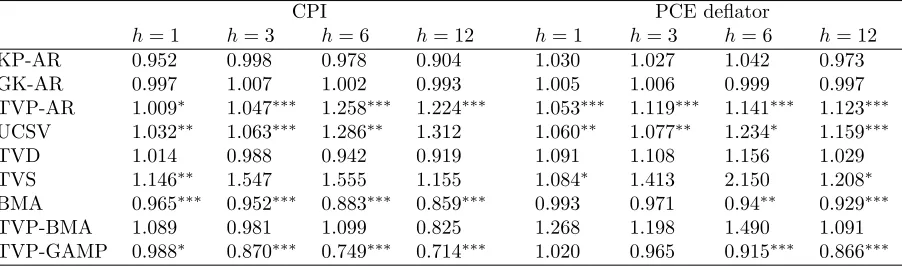
The results from this forecasting exercise are presented in Tables 1 and 2, and are very
encouraging for the proposed TVP-GAMP method. Table 1 shows MSFEs relative to an
AR(2) benchmark (with an intercept), such that numbers lower than one signify better
performance of a competing model relative to that benchmark AR(2) specification. It
can be seen that under the specified regression model, point forecasts from TVP-GAMP
dominate alternatives by a substantial amount, both for CPI and PCE inflation. The
forecast gains are increasing with the horizon. Table 2 shows the logarithm of the average
predictive likelihood (log APL), and this metric is quoted as a spread from the log APL of
the simple AR(2) specification. Positive values signify better performance relative to the
benchmark AR(2). Using this metric, TVP-GAMP is either the top performing model or
Table 1: Point forecast performance: MSFEs relative to AR(2) benchmark.
CPI PCE deflator
h= 1 h= 3 h= 6 h= 12 h= 1 h= 3 h= 6 h= 12
KP-AR 0.952 0.998 0.978 0.904 1.030 1.027 1.042 0.973
GK-AR 0.997 1.007 1.002 0.993 1.005 1.006 0.999 0.997
TVP-AR 1.009∗ 1.047∗∗∗ 1.258∗∗∗ 1.224∗∗∗ 1.053∗∗∗ 1.119∗∗∗ 1.141∗∗∗ 1.123∗∗∗
UCSV 1.032∗∗ 1.063∗∗∗ 1.286∗∗ 1.312 1.060∗∗ 1.077∗∗ 1.234∗ 1.159∗∗∗
TVD 1.014 0.988 0.942 0.919 1.091 1.108 1.156 1.029
TVS 1.146∗∗ 1.547 1.555 1.155 1.084∗ 1.413 2.150 1.208∗
BMA 0.965∗∗∗ 0.952∗∗∗ 0.883∗∗∗ 0.859∗∗∗ 0.993 0.971 0.94∗∗ 0.929∗∗∗
TVP-BMA 1.089 0.981 1.099 0.825 1.268 1.198 1.490 1.091
TVP-GAMP 0.988∗ 0.870∗∗∗ 0.749∗∗∗ 0.714∗∗∗ 1.020 0.965 0.915∗∗∗ 0.866∗∗∗
Model acronyms are as follows: KP-AR:Koop and Potter (2007) structural breaks AR(p) model;
GK-AR:Giordani and Kohn (2008) structural breaks AR(p) model;TVP-AR:Pettenuzzo and
Timmermann (2017) time-varying parameter AR(p) model; UCSV: Stock and Watson (2007)
unobserved components stochastic volatility; TVD: Chan et al. (2012) time-varying dimension
regression TVS: Kalli and Griffin (2014) time-varying sparsity regression BMA: George and
McCulloch (1993) stochastic search variable selection regresison TVP-BMA: Groen et al.
(2012) time-varying Bayesian model averaging model TVP-GAMP: Shrinkage representation
of time-varying parameter regression, with generalized approximate message passing estimation
Next to MSFE values the results of the Diebold-Mariano statistic are presented, with∗ significance at the 10% level; ∗∗ significance at the 5% level; ∗∗∗ significance at the 1% level.
Table 2: Density forecast performance: log APLs relative to AR(2) benchmark.
CPI PCE deflator
h= 1 h= 3 h= 6 h= 12 h= 1 h= 3 h= 6 h = 12 KP-AR 0.090 0.081 0.002 -0.036 0.011 0.074 -0.057 -0.035 GK-AR -0.025 -0.029 0.004 0.037 0.034 0.138 0.056 0.052 TVP-AR 0.118 0.111 0.181 0.067 0.036 0.007 -0.036 -0.029 UCSV 0.161 0.239 0.224 0.144 0.048 0.245 -0.067 0.059 TVD -0.103 -0.005 -0.339 -0.380 -0.097 0.062 -0.885 -0.262 TVS 0.018 -0.163 -0.660 -0.367 -0.001 0.003 -0.427 -0.246 BMA 0.030 -0.067 0.042 0.084 -0.056 -0.002 -0.062 0.030 TVP-BMA 0.121 0.313 0.413 0.399 -0.026 0.227 0.205 0.219 TVP-GAMP -0.204 0.258 0.320 0.321 0.061 0.260 0.045 0.191
See notes in Table 1 for details of model acronyms.
[image:29.612.82.520.467.630.2]parameters is important for inflation. The three models with the largest number of
predictors, namely BMA and TVP-GAMP, and to a lesser degree TVP-BMA, seem to
be improving a lot over time-varying parameter models with no predictors. The results
seem to suggest that information in predictors is more important than the specification
of time variation in regression parameters. This observation is not undermined by the
fact that point forecasts from TVP-BMA are not significant, and that density forecasts
from BMA are quite poor relative to TVP-BMA and TVP-GAMP. First, TVP-BMA is
overparametrized13 its point forecast performance is not as good as the more conservative
(in terms of time-variation in parameters, not available number of predictors) BMA and
TVP-GAMP specifications. Second, when considering density forecasts, BMA is definitely
misspecified since it does not allow for stochastic volatility, and it naturally doesn’t perform
as well as TVP-BMA and TVP-GAMP that allow for changing variance. Therefore, these
findings suggest that TVP-GAMP is overall the best model and that its specification is
flexible enough to capture both structural change and utilize information in a large set
of predictors at the same time. Most importantly, the SBL prior allows to strike a good
balance between these two modeling characteristics by removing irrelevant predictors as
well as regularizing time variation.
These results are in stark contrast to existing results for TVP models presented in the
papers cited above (see e.g. footnotes in Table 1). The culprit is simply the assumption
that inflation is I(1) that Stock and Watson (1999) introduce in their seminal paper, and
that it is adopted in equation (37). Once the random walk dynamics are removed from
inflation (i.e. inflation gap becomes the dependent variable), the role of time-varying
parameters in forecasting becomes less important and the most significant feature is the
information included in exogenous predictors. It would be interesting then, as a robustness
13Shrinkage in TVP-BMA is only across predictors, but this model does not restrict the amount of
check, to specify the forecasting regression for inflation using the following form
πht+h =φt,0 +ftθt(L) +πtµt(L) +et+h. (38)
This equation is more in line with the forecasting model estimated in papers such as Chan
et al. (2012), Groen et al. (2013), or Pettenuzzo and Timmermann (2017).
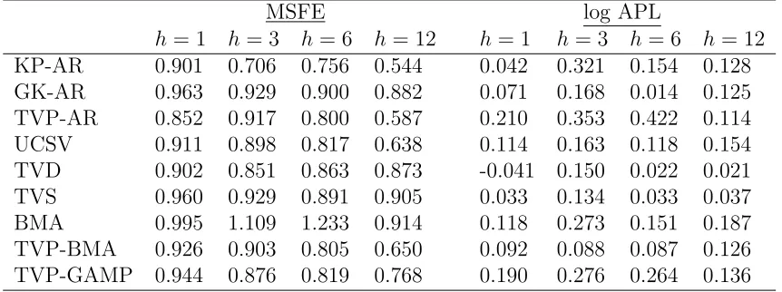
Table 3 shows results based on this alternative specification of equation (38) for CPI
inflation only. The left part of the table presents MSFE results, while the right panel
presents log APLs. In this case it is evident that the various variants of TVP models
considered improve tremendously over the benchmark. As a matter of fact, models such
as the KP-AR, TVP-AR and UCSV also improve a lot relative to the constant parameter
BMA. Looking at point forecasts and the associated MSFE results, we can observe many
differences among TVP models, especially as the forecast horizon increases. For example,
the structural breaks KP-AR specification has the lowest relative MSFE for h = 12
among all models, but the also structural breaks GK-AR specification is among the worst
performing (but still much better than the simple AR model). TVD and TVS estimated
with the monthly data are not only cumbersome, but also do not perform as well as TVP
models with no predictors. In contrast, the TVP-BMA algorithm is performing quite
well, even though it still doesn’t beat TVP models with no predictors. In this alternative
forecasting regression, TVP-GAMP is not the top forecasting model but its performance
is still quite good. If it wasn’t for the exceptional performance of the KP-AR model,
TVP-GAMP would have been a top model forh = 1,3,6.
When looking at density forecast evaluation the results might not comply with the
results for the point forecasts. Still good performing models are the KP-AR and the
TVP-AR, but now the BMA and TVP-GAMP beat models such as the UCSV. With such
density forecasts. Nevertheless, for the forecasting regression (38) it seems that the way
time variation in parameters is specified is more important than information in exogenous
predictors. Further numerical evidence on the relative forecast performance of some of the
[image:32.612.86.517.236.397.2]competing models, is provided in Online Appendix, Section D.2.
Table 3: Point and density forecast performance using alternative definition of the CPI forecasting regression
MSFE log APL
h= 1 h= 3 h= 6 h= 12 h = 1 h= 3 h= 6 h= 12 KP-AR 0.901 0.706 0.756 0.544 0.042 0.321 0.154 0.128 GK-AR 0.963 0.929 0.900 0.882 0.071 0.168 0.014 0.125 TVP-AR 0.852 0.917 0.800 0.587 0.210 0.353 0.422 0.114 UCSV 0.911 0.898 0.817 0.638 0.114 0.163 0.118 0.154 TVD 0.902 0.851 0.863 0.873 -0.041 0.150 0.022 0.021 TVS 0.960 0.929 0.891 0.905 0.033 0.134 0.033 0.037 BMA 0.995 1.109 1.233 0.914 0.118 0.273 0.151 0.187 TVP-BMA 0.926 0.903 0.805 0.650 0.092 0.088 0.087 0.126 TVP-GAMP 0.944 0.876 0.819 0.768 0.190 0.276 0.264 0.136
See notes in Table 1 for details of model acronyms.
Unlike the previous two tables that present results for both CPI and PCE, this table only shows results for CPI, where its left panel focuses on MSFEs and its right panel on log APLs. However, as in the previous two tables, MSFEs and log APLs are relative to an AR(2) benchmark. MSFE entries lower than one mean that the estimation method of the respective row does better than the benchmark. Log APL entries higher than zero mean that the estimation method of the respective row does better than the benchmark.
5
Conclusions
This paper evaluates a new methodology for performing Bayesian inference in
high-dimensional regression models. The proposed Generalized Approximate Message Passing
(GAMP) is a fast algorithm for approximating iteratively the first two moments of the
marginal posterior distribution of a high-dimensional vector of coefficients. It is established
such as hierarchical shrinkage priors, time-varying coefficients and stochastic volatility,
and many predictors. The benefit of the proposed approach is demonstrated using an
inflation forecasting exercise that leads to the recursive estimation of regression models
with thousands of covariates. Due to the low algorithmic complexity, GAMP could be
generalized to much higher dimensions with millions of predictors/covariates, as it is also
trivially parallelizable.
The current study opens up new avenues for research. First, the proposed framework
for modeling time-vayring parameters using hierarchical shrinkage priors can be extended
in interesting ways. For example, shrinkage estimators/priors that apply on group of
coefficients (such as the Group Lasso) can be used in this setting so that coefficients are
shrunk either in groups of predictors for a given time period or in groups of consecutive time
periods for a given predictor. This is because in the TVP setting the vector of regression
coefficients β has elements that correspond both to predictor j, j = 1, ..., p, but also to
time period t, t = 1, ..., T. One can think of other shrinkage priors in order to perform
a more structured approach to uncovering patterns of time-variation in parameters, such
as various pooling priors used in the panel data literature. Finally, the paper proposes
the framework of factor graphs for designing efficient algorithms. Many macroeconomic
problems currently do not typically involve extensive use of Big Data sets, however, they
involve multivariate models with possibly thousands of coefficients, such as VAR, factor,
and DSGE models. Bayesian estimation of these models is quite cumbersome, many times
relying on linear or nonlinear state-space methods. As empirical macroeconomic models
become larger and more complex, factor graph inference could help economists come up
References
[1] Al-Shoukairi, M., Schniter, P. and B. D. Rao (2018). A GAMP-based low complexity
sparse Bayesian learning algorithm. IEEE Transactions on Signal Processing, 66(2),
294-308.
[2] Amir-Ahmadi, P., Matthes, C. and M.-C. Wang (forthcoming). Choosing prior
hyperparameters: With applications to time-varying parameter models. Journal of
Business and Economic Statistics.
[3] Angelino, E., Johnson, M. J. and R. P. Adams (2016). Patterns of scalable Bayesian
inference. Foundations and Trends➤ in Machine Learning, 9(2-3), 119-247.
[4] Barber, D. (2012). Bayesian reasoning and machine learning. Cambridge University
Press: New York.
[5] Bauwens, L., Koop, G., Korobilis, D. and J. V. K. Rombouts (2015). The contribution
of structural break models to forecasting macroeconomic series. Journal of Applied
Econometrics, 30(4), 596-620.
[6] Belmonte, M., Koop, G. and D. Korobilis (2014). Hierarchical shrinkage in
time-varying coefficients models. Journal of Forecasting, 33, 80-94.
[7] Bishop, C. M. (2006).Pattern recognition and machine learning. Springer: New York.
[8] Chan, J., Koop, G., Leon-Gonzalez, R. and R. Strachan (2012). Time varying
dimension models. Journal of Business and Economic Statistics 30(3), 358-367.
[9] Cooley, T. F. and E. C. Prescott (1976). Estimation in the presence of stochastic
[10] Donoho, D. L., Maleki, A. and A. Montanari (2009). Message passing algorithms for
compressed sensing. Proceedings of National Academy of Sciences, 106(45),
18914-18919.
[11] Donoho, D. L., Maleki, A. and A. Montanari (2011). How to design message
passing algorithms for compressed sensing. Unpublished manuscript, available at
http://www.ece.rice.edu/ mam15/bpist.pdf.
[12] Fr¨uhwirth-Schnatter, S. and H. Wagner (2010). Stochastic model specification search
for Gaussian and partial non-Gaussian state space models. Journal of Econometrics
154(1), 85-100.
[13] George, E. I. and R. E. McCulloch (1993). Variable selection via Gibbs sampling.
Journal of the American Statistical Association, 88(423), 881-889.
[14] Giordani, P. and R. Kohn (2008). Efficient Bayesian inference for multiple
change-point and mixture innovation models. Journal of Business and Economic Statistics,
26(1) 66-77.
[15] Groen, J. J. J., Paap, R. and F. Ravazzollo (2013). Real time inflation forecasting in
a changing world. Journal of Business and Economic Statistics, 31(1) 29-44.
[16] Herbst, E. P. and F. Schorfheide (2015). Bayesian estimation of DSGE models.
Princeton University Press: New Jersey.
[17] Jackson, M. O. (2008). Social and economic networks. Princeton University Press:
New Jersey.
[18] Kalli, M. and J. E. Griffin (2014). Time-varying sparsity in dynamic regression models.
[19] Koop, G. and D. Korobilis (2010). Bayesian multivariate time series methods for
empirical macroeconomics. Foundations and Trends➤ in Econometrics 3, pp.
267-358.
[20] Korobilis, D. (2013). Hierarchical shrinkage priors for dynamic regressions with many
predictors. International Journal of Forecasting, 29, 43-59.
[21] Kowal, D. R., Matteson, D. S. and D. Ruppert (2017). Dynamic shrinkage processes.
arXiv:1707.00763.
[22] Kschischang, F. R., Frey, B. J. and H. A. Loeliger (2001). Factor graphs and the
sum-product algorithm. IEEE Transactions on Information Theory, 47(2), 498-519.
[23] Mooij, J. and H. Kappen (2007). Sufficient conditions for convergence of the
sumproduct algorithm.IEEE Transactions on Information Theory, 53(12), 4422-4437.
[24] Nakajima, J. and M. West (2013). Bayesian analysis of latent threshold dynamic
models. Journal of Business and Economic Statistics, 31(2), 151-164.
[25] Pearl, J. (1982). Reverend Bayes on inference engines: A distributed hierarchical
approach. AAAI-82: Pittsburgh, PA. Second National Conference on Artificial
Intelligence. Menlo Park, California: AAAI Press, 133-136.
[26] Pettenuzzo, D. and A. Timmermann (2017). Forecasting macroeconomic variables
under model instability.Journal of Business and Economic Statistics, 35(2), 183-201.
[27] Rangan, S. (2011). Generalized approximate message passing for estimation with
random linear mixing.IEEE International Symposium on Information Theory,
[28] Rangan, S., Schniter, P., Riegler, E., Fletcher, A. K. and V. Cevher (2016).
Fixed points of generalized approximate message passing with arbitrary matrices.
arXiv:1301.6295v4.
[29] Roˇckov´a, V. and K. McAlinn (2018). Dynamic variable selection with spike-and-slab
process priors. Technical report, Booth School of Business, University of Chicago.
[30] Stock, J. H. and M. W. Watson (1999). Forecasting inflation. Journal of Monetary
Economics, 44(2), 293-335.
[31] Stock, J. H. and M. W. Watson (2007). Why has U.S. inflation become harder to
forecast? Journal of Money, Credit and Banking 39, 333.
[32] Tipping, M. E. (2001). Sparse Bayesian learning and the relevance vector machine.
Journal of Machine Learning Research, 1, 211-244.
[33] Vehtari, A., Gelman, A., Sivula, T., Jyl¨anki, P., Tran, D., Sahai, S., Blomstedt,
P., Cunningham, J. P., Schiminovich, D., and C. Robert (2018). Expectation
propagation as a way of life: A framework for Bayesian inference on partitioned
data. arXiv:1412.4869v3.
[34] Wand, M. P. (2017). Fast approximate inference for arbitrarily large semiparametric
regression models via message passing.Journal of the American Statistical Association
112, 137-168.
[35] Zou, X., Li, F., Fang, J. and H. Li(2016). Computationally efficient sparse Bayesian
learning via generalized approximate message passing. IEEE International Conference
Online Appendix to “High-dimensional macroeconomic
forecasting using message passing algorithms”
Dimitris Korobilis
A
Data Appendix
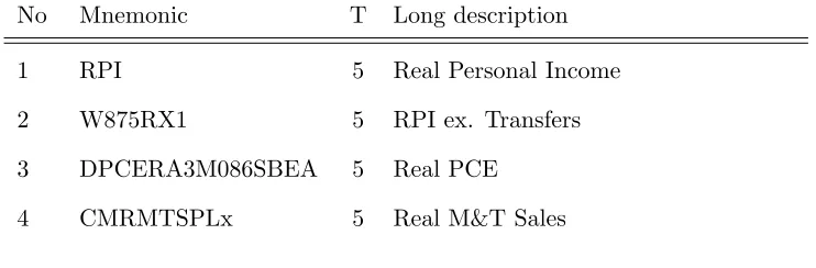
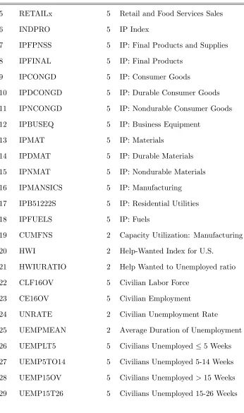
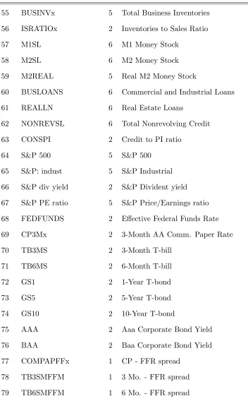
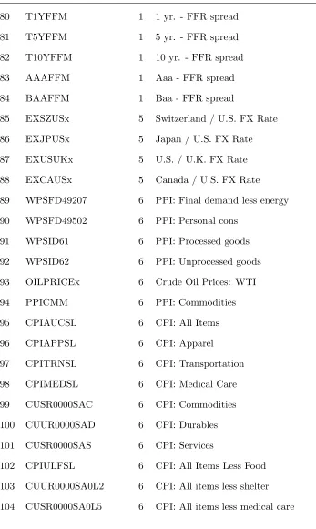
All series were downloaded from Michael McCracken’s FRED-MD database (https :
//research.stlouisf ed.org/econ/mccracken/f red − databases/) and cover the period
1959M1 to 2016M6. All series are seasonally adjusted and all variables are transformed to
be approximately stationary. In particular, if wi,t is the original un-transformed series in
levels, when the series is used as a predictor the transformation codes (column T of the
table) are: 1 - no transformation (levels), xi,t =wi,t; 2 - first difference, xi,t =wi,t−wi,t−1
; 3- second difference, xi,t = ∆wi,t − ∆wi,t−1 4 - logarithm, xi,t = logwi,t; 5 - first
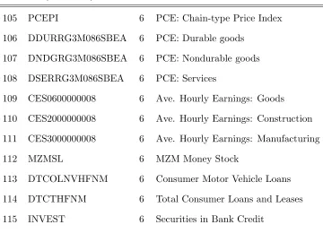
difference of logarithm, xi,t = logwi,t − logwi,t−1; 6 - second difference of logarithm,
[image:38.612.116.487.559.681.2]xi,t = ∆ logwi,t−∆ logwi,t−1.
Table A1: Monthly U.S. macro data set (based on FREDMD)
No Mnemonic T Long description
1 RPI 5 Real Personal Income
2 W875RX1 5 RPI ex. Transfers
3 DPCERA3M086SBEA 5 Real PCE
Table A1 (continued)
5 RETAILx 5 Retail and Food Services Sales
6 INDPRO 5 IP Index
7 IPFPNSS 5 IP: Final Products and Supplies
8 IPFINAL 5 IP: Final Products
9 IPCONGD 5 IP: Consumer Goods
10 IPDCONGD 5 IP: Durable Consumer Goods
11 IPNCONGD 5 IP: Nondurable Consumer Goods
12 IPBUSEQ 5 IP: Business Equipment
13 IPMAT 5 IP: Materials
14 IPDMAT 5 IP: Durable Materials
15 IPNMAT 5 IP: Nondurable Materials
16 IPMANSICS 5 IP: Manufacturing
17 IPB51222S 5 IP: Residential Utilities
18 IPFUELS 5 IP: Fuels
19 CUMFNS 2 Capacity Utilization: Manufacturing
20 HWI 2 Help-Wanted Index for U.S.
21 HWIURATIO 2 Help Wanted to Unemployed ratio
22 CLF16OV 5 Civilian Labor Force
23 CE16OV 5 Civilian Employment
24 UNRATE 2 Civilian Unemployment Rate
25 UEMPMEAN 2 Average Duration of Unemployment
26 UEMPLT5 5 Civilians Unemployed ≤5 Weeks
27 UEMP5TO14 5 Civilians Unemployed 5-14 Weeks
28 UEMP15OV 5 Civilians Unemployed >15 Weeks
[image:39.612.125.471.108.693.2]Table A1 (continued)
30 UEMP27OV 5 Civilians Unemployed >27 Weeks
31 CLAIMSx 5 Initial Claims
32 PAYEMS 5 All Employees: Total nonfarm
33 USGOOD 5 All Employees: Goods-Producing
34 CES1021000001 5 All Employees: Mining and Logging
35 USCONS 5 All Employees: Construction
36 MANEMP 5 All Employees: Manufacturing
37 DMANEMP 5 All Employees: Durable goods
38 NDMANEMP 5 All Employees: Nondurable goods
39 SRVPRD 5 All Employees: Service Industries
40 USTPU 5 All Employees: TT&U
41 USWTRADE 5 All Employees: Wholesale Trade
42 USTRADE 5 All Employees: Retail Trade
43 USFIRE 5 All Employees: Financial Activities
44 USGOVT 5 All Employees: Government
45 CES0600000007 1 Hours: Goods-Producing
46 AWOTMAN 2 Overtime Hours: Manufacturing
47 AWHMAN 1 Hours: Manufacturing
48 HOUST 4 Starts: Total
49 HOUSTNE 4 Starts: Northeast
50 HOUSTMW 4 Starts: Midwest
5