Munich Personal RePEc Archive
Observations on Cooperation
Heller, Yuval and Mohlin, Erik
Bar Ilan Univeristy, Lund University
15 November 2017
Online at
https://mpra.ub.uni-muenchen.de/82740/
Observations on Cooperation
Yuval Heller
∗and Erik Mohlin
†‡November 15, 2017
Final pre-print of a manuscript accepted for publication in the Review of Economic Studies.
Abstract
We study environments in which agents are randomly matched to play a Prisoner’s Dilemma, and each player observes a few of the partner’s past actions against previous opponents. We depart from the existing
related literature by allowing a small fraction of the population to be commitment types. The presence of committed agents destabilizes previously proposed mechanisms for sustaining cooperation. We present a
novel intuitive combination of strategies that sustains cooperation in various environments. Moreover, we show that under an additional assumption of stationarity, this combination of strategies is essentially the
uniquemechanism to support full cooperation, and it is robust to various perturbations. Finally, we extend
the results to a setup in which agents also observe actions played by past opponents against the current
partner, and we characterize which observation structure is optimal for sustaining cooperation.
JEL Classification: C72, C73, D83. Keywords: Community enforcement; indirect reciprocity; random matching; Prisoner’s Dilemma; image scoring.
1
Introduction
Consider the following example of a simple yet fundamental economic interaction. Alice has to trade with another agent, Bob, whom she does not know. Both sides have opportunities to cheat, to their own benefit, at the expense of the other. Alice is unlikely to interact with Bob again, and thus her ability to retaliate, in case Bob acts opportunistically, is restricted. The effectiveness of external enforcement is also limited, e.g., due to incompleteness of contracts, non-verifiability of information, and court costs. Thus cooperation may be impossible to achieve. Alice searches for information about Bob’s past behavior, and she obtains anecdotal evidence about Bob’s actions in a couple of past interactions. Alice considers this information when she decides how to act. Alice also takes into account that her behavior toward Bob in the current interaction may be
∗Affiliation: Department of Economics, Bar Ilan University, Israel. E-mail: [email protected]. †Affiliation: Department of Economics, Lund University, Sweden. E-mail: [email protected].
‡A previous version of this paper was circulated under the title “Stable observable behavior.” We have benefited greatly from
observed by her future partners. Historically, the above-described situation was a challenge to the establishment of long-distance trade (Milgrom, North, and Weingast,1990;Greif,1993), and it continues to play an important role in the modern economy, in both offline (Bernstein,1992;Dixit,2003) and online interactions (Resnick and Zeckhauser,2002;Jøsang, Ismail, and Boyd,2007).
Several papers have studied the question of how cooperation can be supported by means of community enforcement. Most of these papers assume that all agents in the community are rational and, in equilibrium, best reply to what everyone else is doing. As argued by Ellison (1994, p. 578), this assumption may be fairly implausible in large populations. It seems quite likely that, in a large population, there will be at least some agents who fail to best respond to what the others are doing, either because they are boundedly rational, have idiosyncratic preferences, or because their expectations about other agents’ behavior are incorrect. Motivated by this argument, we allow a few agents in the population to be committed to behaviors that do not necessarily maximize their payoffs. It turns out that this seemingly small modification completely destabilizes existing mechanisms for sustaining cooperation when agents are randomly matched with new partners in each period. Specifically, both the contagious equilibria (Kandori,1992;Ellison,1994) and the “belief-free” equilibria (Takahashi,2010;Deb,2012) fail in the presence of a small fraction of committed agents.1
Our key results are as follows. First, we show that always defecting is the unique perfect equilibrium, regardless of the number of observed actions, provided that the bonus of defection in the underlying Prisoner’s Dilemma is larger when the partner cooperates than when the partner defects. Second, in the opposite case, when the bonus of defection is larger when the partner defects than when the partner cooperates, we present a novel and essentially unique combination of strategies that sustains cooperation: all agents cooperate when they observe no defections and defect when they observe at least two defections.2 Some of the agents also defect
when observing a single defection. Importantly, this cooperative behavior is robust to various perturbations, and it appears consistent with experimental data. Third, we extend the model to environments in which an agent also obtains information about the behavior of past opponents against the current partner. We show that in this setup cooperation can be sustained if and only if the bonus of defection of a player is less than half the loss she induces a cooperative partner to suffer. Finally, we characterize an observation structure that allows cooperation to be supported as a perfect equilibrium outcome in all Prisoner’s Dilemma games. In all observation structures we use the same essentially unique construction to sustain cooperation.
Overview of the Model Agents in an infinite population are randomly matched into pairs to play the Prisoner’s Dilemma game, in which each player decides simultaneously whether to cooperate or defect (see the payoff matrix in Table1). If both players cooperate they obtain a payoff of one, if both defect they obtain a payoff of zero, and if one of the players defects, the defector gets 1 +g, while the cooperator gets −l, where
g, l > 0 andg < l+ 1. (The latter inequality implies that mutual cooperation is the efficient outcome that maximizes the sum of payoffs.)
Before playing the game, each agent privately draws a random sample of k actions that have been played by her partner against other opponents in the past. The assumption that a small random sample is taken from the entire history of the partner is intended to reflect a setting in which the memory of past interactions is long
1In contagious equilibria players start by cooperating. If one player defects at staget, her partner defects at staget+ 1, infecting
another player who defects at staget+ 2, and so on. In belief-free equilibria players are always indifferent between their actions, but they choose different mixed actions depending on the signal they obtain about the partner. We discuss the non-robustness of these classes of equilibria at the end of Section4.2.
2As discussed later, our uniqueness results also rely on an additional assumption that agents are restricted to choose stationary
Table 1: Matrix Payoffs of Prisoner’s Dilemma Games
c d
c 1 1 −l 1+g
d 1+g −l 0 0
g, l >0 , g < l+ 1
and accurate but dispersed. This means that the information that reaches an agent about her partner (through gossip) arrives in a non-deterministic fashion and may stem from any point in the past.
We require each agent to follow a stationary strategy, i.e., a mapping that assigns a mixed action to each signal that the agent may observe about the current partner. (That is, the action is not allowed to depend on calendar time or on the agent’s own history.) Asteady state of the environment is a pair consisting of: (1) a distribution of strategies with a finite support that describes the fractions of the population following the different strategies, and (2) asignal profile that describes the distribution of signals that is observed when an agent is matched with a partner playing any of the strategies present in the population. The signal profile is required to beconsistent with the distribution of strategies in the sense that a population of agents who follow the distribution of strategies and observe signals about the partners sampled from the signal profile will behave in a way that induces the same signal profile.3
Our restriction to stationary strategies and our focus on consistent steady states allow us to relax the standard assumption that there is an initial time zero at which an entire community starts to interact. In various real-life situations, the interactions within the community have been going on from time immemorial. Consequently the participants may have only a vague idea of the starting point. Arguably, agents might therefore be unable to condition their behavior on everything that has happened since the beginning of the interactions.
We perturb the environment by introducing ǫ committed agents who each follow one strategy from an arbitrary finite set ofcommitment strategies. We assume that at least one of the commitment strategies is totally mixed, which implies that all signals (i.e., all sequences ofk actions) are observed with positive probability. A steady state in a perturbed environment describes a population in which 1−ǫof the agents are normal; i.e., they play strategies that maximize their long-run payoffs, whileǫof the agents follow commitment strategies.
We adapt the notions of Nash equilibrium and perfect equilibrium (Selten, 1975) to our setup. A steady state is aNash equilibriumif no normal agent can gain in the long run by deviating to a different strategy (the agents are assumed to be arbitrarily patient). The deviator’s payoff is calculated in the new steady state that emerges following her deviation. A steady state is aperfect equilibrium if it is the limit of a sequence of Nash equilibria in a converging sequence of perturbed environments.4
3
The reason why the consistent signal profile is required to be part of the description of a steady state, rather than being uniquely determined by the distribution of strategies, is that our environment, unlike a standard repeated game, lacks a global starting time that determines the initial conditions. An example of a strategy that has multiple consistent signal profiles is as follows. The parameterkis equal to three, and everyone plays the most frequently observed action in the sample of the three observed actions. There are three behaviors that are consistent with this population: one in which everyone cooperates, one in which everyone defects, and one in which everyone plays (on average) uniformly.
4In AppendixDwe show that all the equilibria presented in this paper satisfy two additional refinements: (1) evolutionary
stability (Maynard Smith,1974) – any small group of agents who jointly deviate are outperformed, and (2)robustness– no small
Summary of Results We start with a simple result (Prop. 1) that shows that defection is a perfect equili-brium outcome for any number of observed actions.
We say that a Prisoner’s Dilemma game is offensive if there is a stronger incentive to defect against a cooperator than against a defector (i.e., g > l); in a defensive Prisoner’s Dilemma the opposite holds (i.e.,
g < l). Our first main result (Theorem1) shows that always defecting is the unique perfect equilibrium in any offensive Prisoner’s Dilemma game (i.e.,g > l) for any number of observed actions. The result assumes a mild regularity condition on the set of commitment strategies (Def. 3), namely, that this set is rich enough that, in any steady state of the perturbed environment, at least one of the commitment strategies induces agents to defect with a different probability than that of some of the normal agents. The intuition is as follows. The mild assumption that not all agents defect with exactly the same probability implies that the signal that Alice observes about her partner Bob is not completely uninformative. In particular, the more often Alice observes Bob to defect, the more likely Bob will defect against Alice. In offensive games, it is better to defect against partners who are likely to cooperate than to defect against partners who are likely to defect. This implies that a deviator who always defects is more likely to induce normal partners to cooperate. Consequently, such a deviator will outperform any agent who cooperates with positive probability.
Theorem 1 may come as a surprise in light of a number of existing papers that have presented various equilibrium constructions that support cooperation in any Prisoner’s Dilemma game that is played in a po-pulation of randomly matched agents. Our result demonstrates that, in the presence of a small fraction of committed agents, the mechanisms that have been proposed to support cooperation fail, regardless of how these committed agents play (except in the “knife-edge” case ofg=l; seeDilmé,2016and Remark7in Section4.3). Thus, our paper provides an explanation of why experimental evidence suggests that subjects’ behavior corre-sponds neither to contagious equilibria (see, e.g.,Duffy and Ochs,2009) nor to belief-free equilibria (see, e.g., Matsushima, Tanaka, and Toyama, 2013). The empirical predictions of our model are discussed in Appendix B.
Our second main result (Theorem2) shows that cooperation is a perfect equilibrium outcome in any defensive Prisoner’s Dilemma game (g < l) when players observe at least two actions. Moreover, there is an essentially unique distribution of strategies that support cooperation, according to which: (a) all agents cooperate when observing no defections, (b) all agents defect when observing at least 2 defections, (c) the normal agents defect with an average probability of 0< q <1 when observing a single defection. The intuition for the result is as follows. Defection yields a direct gain that is increasing in the partner’s probability of defection (due to the game being defensive). In addition, defection results in an indirect loss because it induces future partners to defect when they observe the current defection. This indirect loss is independent of the current partner’s behavior. One can show that there always exists a probabilityqsuch that the above distribution of strategies balances the direct gain and the indirect loss of defection, conditional on the agent observing a single defection. Furthermore, cooperation is the unique best reply conditional on the agent observing no defections, and defection is the unique best reply conditional on the agent observing at least two defections.
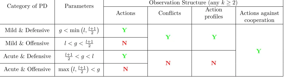
Observations Based on Action Profiles So far we have assumed that each agent observes only the partner’s (Bob’s) behavior against other opponents, but that she cannot observe the behavior of the past opponents against Bob. In Section 5 we relax this assumption. Specifically, we study three observation structures: the first two seem to be empirically relevant, and the third one is theoretically important since it allows us to construct an equilibrium that sustains cooperation in all Prisoner’s Dilemma games.
1. Observing conflicts: Each agent observes, in each of thek sampled interactions of her partner, whether there was mutual cooperation (i.e., no conflict: both partners are “happy”) or not (i.e., partners complain about each other, but it is too costly for an outside observer to verify who actually defected). Such an observation structure (which we have not seen described in the existing literature) seems like a plausible way to capture non-verifiable feedback about the partner’s behavior.
2. Observing action profiles: Each agent observes the full action profile in each of the sampled interactions.
3. Observing actions against cooperation: Each agent observes, in each of the sampled interactions, what action the partner took provided that the partner’s opponent cooperated. If the partner’s opponent defected then there is no information about what the partner did.
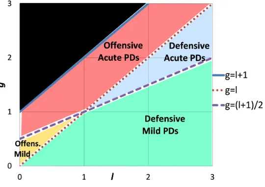
It turns out that the stability of cooperation in the first two observation structures crucially depends on a novel classification of Prisoner’s Dilemma games. We say that a Prisoner’s Dilemma game isacute ifg > l+1
2 ,
andmild ifg < l+1
2 . The threshold between the two categories, namely, g=
l+1
2 , is characterized by the fact
that the gain from a single unilateral defection is exactly half the loss incurred by the partner who is the sole cooperator. Consider a setup in which an agent is deterred from unilaterally defecting because it induces future partners to unilaterally defect against the agent with some probability. Deterrence in acute Prisoner’s Dilemmas requires this probability to be more than 50%, while a probability of below 50% is enough to deter deviations in mild PDs. Figure1(in Section5.2) illustrates the classification of Prisoner’s Dilemma games.
Our next results (Theorems3–4) show that in both observation structures (conflicts or action profiles, and anyk≥2) cooperation is a perfect equilibrium outcome if and only if the underlying Prisoner’s Dilemma game is mild. Moreover, cooperation is supported by essentially the same unique behavior as in Theorem 2. The intuition for why cooperation cannot be sustained in acute games with observation of conflicts is as follows. In order to support cooperation agents should be deterred from defecting against cooperators. As discussed above, in acute games, such deterrence requires that each such defection induce future partners to defect with a probability of at least 50%. However, this requirement implies that defection is contagious: each defection by an agent makes it possible that future partners observe a conflict both when being matched with the defecting agent and when being matched with the defecting agent’s partner. Such future partners defect with a probability of at least 50% when making such observations. Thus the fraction of defections grows steadily, until all normal agents defect with high probability.
Finally, we show that the third observation structure,observing actions against cooperation, is optimal in the sense that it sustains cooperation as a perfect equilibrium outcome for any Prisoner’s Dilemma game (Theorem 5). The intuition for this result is that not allowing Alice to observe Bob’s behavior against a defector helps to sustain cooperation because it implies that defecting against a defector does not have any negative indirect effect (in any steady state) because it is never observed by future opponents. This encourages agents to defect against partners who are more likely to defect (regardless of the values ofg andl).
Conventional Model and Unrestricted Strategies In AppendixA, we relax the assumption that agents are restricted to choosing only stationary strategies. We present a conventional model of repeated games with random matching that differs from the existing literature only by our introducing a few committed agents. We show that this difference is sufficient to yield most of our key results.
Specifically, the characterization of the conditions under which cooperation can be sustained as a perfect equilibrium outcome (as summarized in Table 1 in Section 5.3) holds also when agents are not restricted to stationary strategies, and even when agents observe the most recent past actions of the partner. On the other hand, the relaxation of the stationarity assumption in AppendixAweakens the uniqueness results of the main model in two respects: (1) rather than showing that defection is the unique equilibrium outcome in offensive games, we show only that it is impossible to sustain full cooperation in such games; and (2) while a variant of the simple strategy of the main model still supports cooperation when the set of strategies is unrestricted, we are no longer able to show that this strategy is the unique way to support full cooperation.
Structure Section2presents the model. Our solution concept is described in Section3. Section4studies the observation of actions. Section5extends the model to deal with general observation structures. We discuss the related literature in Section6, and conclude in Section7. AppendixAadapts our key result to a conventional model with an unrestricted set of strategies. Appendix B discusses our empirical predictions. Appendix C presents technical definitions. In Appendix D we present the refinements of strict perfection, evolutionary stability, and robustness. The formal proofs appear in Appendix E. Appendix F studies the introduction of cheap talk to our setup. The appendices are available online in the supplementary material.
2
Stationary Model
2.1
Environment
We model an environment in which patient agents in a large population are randomly matched in each round to play a two-player symmetric one-shot game. For tractability we assume throughout the paper that the population is a continuum.5 We further assume that the agents are infinitely lived and do not discount the
future (i.e., they maximize the average per-round long-run payoff). Alternatively, our model can be interpreted as representing interactions between finitely lived agents who belong to infinitely lived dynasties, such that an agent who dies is succeeded by a protégé who plays the same strategy as the deceased mentor, and each agent observeskrandom actions played by the partner’s dynasty.
5The results can be adapted to a setup with a large finite population. We do not formalize a large finite population, as this
Before playing the game, each agent (she) privately observeskrandom actions that her partner (he) played against other opponents in the past. As described in detail below, agents are restricted to using only stationary strategies, such that each agent’s behavior depends only on the signal about the partner, and not on the agent’s own past play or on time. Thus, if all agents observe signals that come from a stationary distribution then the agents’ behavior will result in a well-defined aggregate distribution of actions that is also stationary. We focus on steady states of the population, in which the distribution of actions, and hence the distribution of signals, is indeed stationary. In such steady states, the k actions that an agent observes about her partner are drawn independently from the partner’s stationary distribution of actions. This sampling procedure may be interpreted as the limit of a process in which each agent randomly observesk actions that are uniformly sampled from the lastninteractions of the partner, asn→ ∞.
To simplify the notation, we assume that the underlying game has two actions, though all our concepts are applicable to games with any finite number of actions. An environment is a pair E = (G, k), where
G= (A={c, d}, π) is a two-player symmetric normal-form game, andk∈Nis the number of observed actions.
Letπ:A×A→Rbe the payoff function of the underlying game. We refer to actionc(resp.,d) ascooperation
(resp., defection), since we will focus on the Prisoner’s Dilemma in our results. Let ∆ (A) denote the set of mixed actions (distributions overA), and letπbe extended to mixed actions in the usual linear way. We use the lettera(resp.,α) to denote a typical pure (mixed) action. With a slight abuse of notation leta∈Aalso denote the element in ∆ (A) that assigns probability 1 toa. We adopt this convention for all probability distributions throughout the paper.
2.2
Stationary Strategy
The signal observed about the partner is the number of times he played each actiona∈A in the sample ofk
observed actions. LetM ={0, ..., k} denote the set of feasible signals, where signal m∈ M is interpreted as the number of times that the partner defected in the sampledkobservations.6
Given a distribution of actionsα∈∆ (A) and an environmentE = (G, k), letνα(m) be the probability of
an agent observing signalmconditional on being matched with a partner who plays on average the distribution of actionsα. That is,ν(α) :=να∈∆ (M) is a binomial signal distribution that describes a sample ofki.i.d.
actions, where each action is distributed according toα:
∀(m)∈M, να(m) =
k!·(α(d))m·(α(c))(k−m)
m!·(k−m)! . (1)
Astationary strategy(henceforth,strategy)is a mappings:M →∆ (A) that assigns a mixed action to each possible signal. Letsm∈∆ (A) denote the mixed action assigned by strategysafter observing signalm. That
is, for each actiona∈A,sm(a) =s(m) (a) is the probability that a player who follows strategysplays action
aafter observing signalm. We also letadenote the strategysthat plays actionaregardless of the signal, i.e.,
sm(a) = 1 for all m∈M. Strategys istotally mixed, if for each action a∈A, and signal m∈M sm(a)>0.
LetS denote the set of all strategies. Given strategysand distribution of signalsν∈∆ (M), let s(ν)∈∆ (A) be the distribution of actions played by an agent who follows strategysand observes a signal sampled from ν:
∀a∈A, s(ν) (a) = X
m∈M
ν(m)·sm(a).
6We do not allow agents to manipulate the observed signals. In our companion paper (Heller and Mohlin,2016) we study a
2.3
Signal Profile and Steady State
Fix an environment and a finite set of strategiesS. Asignal profileθ:S→∆ (M)is a function that assigns a distribution of signals for each strategy inS. We interpret θs(m) as the probability that signalmis observed
when a partner playing strategysis encountered. LetOS be the set of all signal profiles defined overS. Given
a strategyσ∈∆ (S) and a signal profileθ ∈OS, letθσ ∈∆ (M) be theaverage distribution of signals in the
population, i.e.,θσ(m) :=Ps∈Sσ(s)·θs(m).
We say that a signal profileθ:S→∆ (M) isconsistent with distribution of strategiesσ∈∆ (S) if
∀m∈M, s∈S, θs(m) =ν(s(θσ)) (m). (2)
The interpretation of the consistency requirement is that a population of agents who follow the distribution of strategies σ and observe signals about the partners sampled from the profile θ have to behave in a way that induces the same profile of signal distributions θ. Specifically, when Alice, who follows strategy s, is being matched with a random partner whose strategy is sampled according toσ, she observes a random signal according to the “current” average distribution of signals in the populationθσ. As a result her distribution of
actions iss(θσ), and thus her behavior induces the signal distributionν(s(θσ)). Consistency requires that this
induced signal distribution coincide withθs.
A steady state is a triple consisting of (1) a finite set of strategiesS interpreted as the strategies that are played by the agents in the population, (2) a distributionσover S interpreted as a description of the fraction of agents following each strategy, and (3) a consistent signal profileθ:S→∆ (M). Formally:
Definition 1. Asteady state (orstatefor short) of an environment (G, k) is a triple (S, σ, θ) whereS⊆ S is a finite set of strategies,σ∈∆ (S) is a distribution with full support overS, andθ:S→∆ (M) is a consistent signal profile.
When the set of strategies is a singleton, i.e.,S={s}, we omit the degenerate distribution assigning a mass of one tos, and we write the steady state as a pair ({s}, θ).We adopt this convention, of omitting reference to degenerate distributions, throughout the paper.
A standard argument shows that any distribution of strategies admits a consistent signal profile (Lemma 1 in AppendixC). Some distributions induce multiple consistent profiles of signal distributions. For example, suppose that k = 3, and everyone follows the strategy of playing the most frequently observed action (i.e., defecting iffm≥2). In this setting there are three consistent signal profiles: one in which everyone cooperates, one in which everyone defects, and one in which everyone plays (on average) uniformly7.
2.4
Perturbed Environment
As discussed in the Introduction, and as argued byEllison (1994, p. 578), it seems implausible that in large populations all agents are rational and know exactly the strategies played by other agents in the community. Motivated by this observation, we introduce the notion of a perturbed environment in which a small fraction of agents in the population are committed to playing specific strategies, even though these strategies are not necessarily payoff-maximizing.
A perturbed environment is a tuple consisting of (1) an environment, (2) a distribution λ over a set of commitment strategies SC that includes a totally mixed strategy, and (3) a numberǫ representing the share
7
of agents who are committed to playing strategies inSC (henceforth,committed agents). The remaining 1−ǫ
share of the agents can play any strategy inS (henceforth,normal agents). Formally:
Definition 2. A perturbed environment is a tupleEǫ= (G, k), SC, λ, ǫ, whereGis the underlying game,
k∈Nis the number of observed actions,SCis a non-empty finite set of strategies (called,commitment strategies)
that includes a totally mixed strategy, λ ∈ ∆ SC
is a distribution with full support over the commitment strategies, andǫ≥0 is the mass of committed agents in the population.
We requireSCto include at least one totally mixed strategy because we want all signals to be observed with
positive probability in a perturbed environment whenǫ >0. (This is analogous to the requirement inSelten, 1975, that all actions be played with positive probability in the perturbations defining a perfect equilibrium.)
Throughout the paper we look at the limit in which the share of committed agents, ǫ, converges to zero. This is the only limit taken in the paper. We use the notation ofO(ǫ) (resp., O ǫ2
) to refer to functions that are in the order of magnitude ofǫ(resp.,ǫ2), i.e., f(ǫ)
ǫ →ǫ→00 (resp., f(ǫ)
ǫ2 →ǫ→00).
We refer to SC, λ
as a distribution of commitments. With a slight abuse of notation, we identify an unperturbed environment (G, k), SC, λ
, ǫ= 0
with the equivalent environment (G, k).
Remark 1. To simplify the presentation, the definition of perturbed environment includes only commitment strategies, and it does not allow “trembling hand” mistakes. As discussed in Remark6in Section4.3, the results also hold in a setup in which agents also tremble, as long as the probability by which a normal agent trembles is of the same order of magnitude as the frequency of committed agents.
One of our main results (Theorem1) requires an additional mild assumption on the perturbed environment that rules out the knife-edge case in which all agents (committed and non-committed alike) behave exactly the same. Specifically, a set of commitments is regular if for each distribution of actionsα, there exists a committed strategysthat does not play distributionαwhen observing the signal distribution induced byα. Formally:
Definition 3. A set of commitment strategiesSC isregular if for each distribution of actionsα∈∆ (A), there
exists a strategys∈SC such thats
ν(α)6=α.
If the set of commitments is regular, then we say that the distribution SC, λ
and the perturbed environment (G, k), SC, λ
, ǫ
are regular. An example of a regular set of commitments is the set that includes strategies
s≡α1 ands′≡α2that induce agents to play mixed actionsα16=α2regardless of the observed signal.
2.5
Steady State in a Perturbed Environment
Fix a perturbed environment Eǫ = (G, k), SC, λ, ǫ and a finite set of strategies SN, interpreted as the
strategies followed by the normal agents in the population. We redefine asignal profile θ:SC∪SN →∆ (M)
as a function that assigns a binomial distribution of signals to each strategy inSC∪SN.
Given a distribution over strategies of the normal agents σ ∈ ∆ SN
and a signal profile θ ∈ OSC∪SN, let θ((1−ǫ)·σ+ǫ·λ) ∈ ∆ (M) be the average distribution of signals in the population, i.e., θ((1−ǫ)·σ+ǫ·λ)(m) := P
s∈SC∪SN((1−ǫ)·σ+ǫ·λ) (s)·θs(m). We adapt the definitions of a consistent signal profile and of a steady
state to perturbed environments. This straightforward adaptation is presented in detail in AppendixC. The following example demonstrates a specific steady state in a specific perturbed environment. The example is intended to clarify the various definitions of this section and, in particular, the consistency requirement. Later, we revisit the same example to explain the essentially unique perfect equilibrium that supports cooperation.
Example 1. Consider the perturbed environment ((G, k= 2),({su≡0.5}), ǫ), in which each agent observes
0< ǫ <<1 of committed agents, who choose each action with probability 0.5 regardless of the observed signal. Let S=
s1, s2 , σ= 1 6,
5 6
, θ
be the following steady state. The state includes two normal strategies: s1
ands2. The strategys1 defects iffm≥1, and the strategy s2 defects iffm≥2. The distributionσassigns a
mass of 1 6 tos
1 and a mass of 5 6 tos
2. The consistent signal profileθis defined as follows (neglecting terms of
O ǫ2
throughout the example):
θsu(m) =
25% if m= 0
50% if m= 1
25% if m= 2,
θs1(m) =
1−3.5·ǫ if m= 0
3.5·ǫ if m= 1
0 if m= 2
θs2(m) =
1−0.5·ǫ if m= 0
0.5·ǫ if m= 1
0 if m= 2.
(3)
To confirm the consistency ofθ, we have first to calculate the average distribution of signals in the population:
θ((1−ǫ)·σ+ǫ·λ)(m) =
1−1.75·ǫ if m= 0
1.5·ǫ if m= 1
0.25·ǫ if m= 2.
Usingθ((1−ǫ)·σ+ǫ·λ), we confirm the consistency ofθs1 andθ
s2 (the consistency ofθ
suis immediate). We do so by calculating distribution of actions played by a player following strategysi who observes the distribution of
actions of a random partner:
s1 θ
((1−ǫ)·σ+ǫ·λ)(c) = 1−1.75·ǫ
s1 θ
((1−ǫ)·σ+ǫ·λ)
(d) = 1.75·ǫ
s2 θ
((1−ǫ)·σ+ǫ·λ)(c) = 1−0.25·ǫ,
s2 θ
((1−ǫ)·σ+ǫ·λ)
(d) = 0.25·ǫ.
Note that s1 θ
((1−ǫ)·σ+ǫ·λ)
(d) = 1−θ((1−ǫ)·σ+ǫ·λ)(2·c) and s2 θ((1−ǫ)·σ+ǫ·λ)
(d) = θ((1−ǫ)·σ+ǫ·λ)(2·d).
The final step in showing that θ is a consistent profile is the observation that each θsi coincides with the binomial distribution that is induced bysi θ
((1−ǫ)·σ+ǫ·λ)
.
2.6
Discussion of the Model
Our model differs from most of the existing literature on community enforcement in three key dimensions (see, e.g.,Kandori, 1992;Ellison,1994; Dixit, 2003;Deb,2012; Deb and González-Díaz, 2014). In what follows we discuss these three key differences, and their implications on our results.
1. The presence of a few committed agents. If one removes the commitment types from our setup, then one can show (by using belief-free equilibria, as inTakahashi,2010) that: (1) it is always possible to support full cooperation as an equilibrium outcome, and (2) there are various strategies that sustain full cooperation. The results of this paper show that the introduction of a few committed agents, regardless of how they behave, implies very different results: (1) defection is theuniqueequilibrium payoff in offensive Prisoner’s Dilemmas (Theorem 1), and (2) there is an essentially unique strategy combination that supports a cooperative equilibrium in defensive Prisoner’s Dilemmas. The intuition is that the presence of committed agents implies that observation of past actions must have some influence on the likely behavior of the partner in the current match (more detailed discussions of this issue follow Theorem1and Remark 10).
were played in the past, nor on the agent’s own history of play, nor on calendar time. The assumption simplifies the presentation of the model and results. In addition, the assumption allows us to achieve uniqueness results that might not hold without stationarity (as discussed in SectionA.3).
3. Not having a “global time zero.” Most of the existing literature represents interactions within a community as a repeated game that has a “global time zero,” in which the first ever interaction takes place. In many real-life situations, the interactions within a community began a long time ago and have continued, via overlapping generations, to the present day. It seems implausible that today’s agents condition their behavior on what happened in the remote past (or on calendar time). For example, trade interactions have been been taking place from time immemorial. It seems unreasonable to assume that Alice’s behavior today is conditioned on what transpired in some long-forgotten timet= 0, when, say, two hunter-gatherers were involved in the first ever trade. We suggest that, even though real-world interactions obviously begin at some definite date, a good way of modeling what the interacting agents think about the situation may be to get rid of global time zero and focus on strategies that do not condition on what happened in the remote past. The lack of a global time zero is the reason why, unlike in repeated games, a distribution of strategies does not uniquely determine the behavior and the payoffs of the agent, so that one must explicitly add the consistent signal profileθ as part of the description of the state of the population. It is possible to interpret a steady state (S, σ, θ) as a kind of initial condition for society, in which agents already have a long-existing past. That is, we begin our analysis of community interaction at a point in time when agents have for a long time followed the strategy distribution (S, σ) yielding the consistent signal profileθ. We then ask whether any patient agent has a profitable deviation from her strategy. If not, then the steady state (S, σ, θ) is likely to persist. This approach stands in contrast to the standard approach that studies whether or not agents have a profitable deviation at a timet >>1 following a long history that started with the first ever interaction att= 0.
In Appendix A we present a conventional repeated game model that differs from the existing literature in only one key aspect: the presence of a few committed agents. In particular, this alternative model features standard calendar time, and agents discount the future, observe the most recent past actions of the partner, and are not limited to choosing only stationary strategies. We show that most of our results hold also in this setup. We feel that this alternative model, while being closer to the existing literature than the main model, suffers from added technical complexity that may hinder the model from being insightful and accessible.
3
Solution Concept
3.1
Long-Run Payoff
In this subsection we define the long-run average (per-round) payoff of a patient agent who follows a stationary strategys, given a steady state SN, σ, θ
of a perturbed environment (G, k), SC, λ
, ǫ
. The same definition, when takingǫ= 0, holds for an unperturbed environment.
We begin by extending the definition of a consistent signal profile θ to non-incumbent strategies. For each non-incumbent strategy ˆs ∈ S\ SN∪SC
, define θ(ˆs) = θsˆas the distribution of signals induced by a
deviating agent who follows strategy ˆsand observes the distribution of signals induced by a random partner in the population (sampled according to (1−ǫ)·σ(s′) +ǫ·λ(s′)). That is, for each strategy ˆs∈ S\ S∪SC
, and each signalm∈M, we define
θˆs(m) = ν s θˆ ((1−ǫ)·σ+ǫ·λ)
We define the long-run payoff of an agent who follows an arbitrary strategys∈ S as:
πs SN, σ, θ
= X
s′∈SN∪SC
((1−ǫ)·σ(s′) +ǫ·λ(s′))·
X (a,a′)∈A×A
sθ(s′)(a)·s′
θ(s)(a′)·π(a, a′)
. (4)
Eq. (4) is straightforward. The inner (right-hand) sum (i.e.,P
(a,a′)∈A×Asθ(s′)(a)·s′
θ(s)(a′)·π(a, a′)) calculates
the expected payoff of Alice who follows strategys conditional on being matched with a partner who follows strategy s′. The outer sum weighs these conditional expected payoffs according to the frequency of each
incumbent strategy s′ (i.e., ((1−ǫ)·σ(s′) +ǫ·λ(s′))), which yields the expected payoff of Alice against a
random partner in the population.
Letπ(S, σ, θ) be the average payoff of the normal agents in the population:
π SN, σ, θ
= X
s∈SN
σ(s)·πs SN, σ, θ.
3.2
Nash and Perfect Equilibrium
A steady state is a Nash equilibrium if no agent can obtain a higher payoff by a unilateral deviation. Formally:
Definition 4. The steady state SN, σ, θ
of perturbed environment (G, k), SC, λ
, ǫ
is a Nash equilibrium if for each strategys∈ S, it is the case thatπs SN, σ, θ
≤π SN, σ, θ
.
Note that the 1−ǫ normal agents in such a Nash equilibrium must obtain the same maximal payoff. That is, each normal strategys∈SN satisfiesπ
s SN, σ, θ
=π SN, σ, θ
≥πs′ SN, σ, θ for each strategys′ ∈ S.
However, theǫcommitted agents may obtain lower payoffs.
A steady state is a (regular) perfect equilibrium if it is the limit of Nash equilibria of (regular) perturbed environments when the frequency of the committed agents converges to zero. Formally (where the standard definitions of convergence of strategies, distributions and states is presented in AppendixC):
Definition 5. A steady state (S∗, σ∗, θ∗) of the environment (G, k) is a(regular) perfect equilibriumif there exist
a (regular) distribution of commitments SC, λ
and converging sequences SN
n , σn, θnn →n→∞ (S∗, σ∗, θ∗)
and (ǫn>0)n →n→∞ 0, such that for each n, the state SnN, σn, θn
is a Nash equilibrium of the perturbed environment (G, k), SC, λ
, ǫn. In this case, we say that (S∗, σ∗, θ∗) is a (regular) perfect equilibrium with
respect to distribution of commitments SC, λ
. If θ∗ ≡a , we say that action a ∈ A is a (regular) perfect
equilibrium action.
By standard arguments, any perfect equilibrium is a Nash equilibrium of the unperturbed environment. In AppendixC.4we show that any symmetric (perfect) Nash equilibrium of the underlying game corresponds to a (perfect) Nash equilibrium of the environment in which all normal agents ignore the observed signal.
3.3
Stronger Refinements of Perfect Equilibrium
The notion of perfect equilibrium might be considered too weak because it may crucially depend on a specific set of commitment strategies. The refinement of strict perfection (`a laOkada, 1981) requires the equilibrium outcome to be sustained regardless of which commitment strategies are present in the population.
The notion of perfect equilibrium considers only deviations by a single agent (who has mass zero in the infinite population). The refinement of anevolutionarily stable strategy (`a la Maynard Smith and Price, 1973) requires stability against a group of agents with a small positive mass who jointly deviate.
The outcome of a perfect equilibrium may be non-robust in the sense that small perturbations of the distribution of observed signals may induce a change of behavior that moves the population away from the consistent signal profile. We address this issue by introducing a refinement that we call robustness, which requires that if we slightly perturb the distribution of observed signals, then the agents still play the same equilibrium outcome with a probability very close to one (in the spirit of the notion of Lyapunov stability).
4
Prisoner’s Dilemma and Observation of Actions
4.1
The Prisoner’s Dilemma
Our results focus on environments in which the underlying game is the Prisoner’s Dilemma (denoted byGP D),
[image:14.612.94.520.428.525.2]which is described in Table 2. The class of Prisoner’s Dilemma games is fully described by two positive parametersgandl. The two actions are denotedcandd, representing cooperation and defection, respectively. When both players cooperate they both get a high payoff (normalized to one), and when they both defect they both get a low payoff (normalized to zero). When a single player defects he obtains a payoff of 1 +g (i.e., an additional payoff ofg) while his opponent gets−l.
Table 2: Matrix Payoffs of Prisoner’s Dilemma Games
c d
c 1 1 −l 1+g
d 1+g −l 0 0
Prisoner’s Dilemma
GP D: g, l >0 , g < l+ 1
c d
c 1 1 −3 2
d 2 −3 0 0
Ex. 1: Defensive PD
GD: 1 =g < l= 3
c d
c 1 1 −1.7 3.3
d 3.3 −1.7 0 0
Ex. 2: Offensive PD
GO: 2.3 =g > l= 1.7
FollowingDixit(2003) we classify Prisoner’s Dilemma games into two kinds: offensive and defensive.8 In an
offensivePrisoner’s Dilemma there is a stronger incentive to defect against a cooperator than against a defector (i.e., g > l); in adefensive PD the opposite holds (i.e., l > g). If cooperating is interpreted as exerting high effort, then the defensive PD exhibits strategic complementarity; increasing one’s effort from low to high is less costly if the opponent exerts high effort.
4.2
Stability of Defection
We begin by showing that defection is a regular perfect equilibrium action in any Prisoner’s Dilemma game and for anyk. Formally:
8
Proposition 1. LetE= (GP D, k)be an environment. Defection is a regular perfect equilibrium action.
The intuition is straightforward. Consider any distribution of commitment strategies. Consider the steady state in which all the normal incumbents defect regardless of the observed signal. It is immediate that this strategy is the unique best reply to itself. This implies that if the share of committed agents is sufficiently small, then always defecting is also the unique best reply in the slightly perturbed environment.
Our first main result shows that defection is theunique regular perfect equilibrium in offensive games.
Theorem 1. Let E= (GP D, k) be an environment, whereGis an offensive Prisoner’s Dilemma (i.e.,g > l).
If(S∗, σ∗, θ∗)is a regular perfect equilibrium, then S∗={d} andθ∗=k.
Sketch of Proof. The payoff of a strategy can be divided into two components: (1) adirectcomponent: defecting yields additional g points if the partner cooperates and additional l points if the partner defects, and (2) an indirect component: the strategy’s average probability of defection determines the distribution of signals observed by the partners, and thereby determines the partner’s probability of defecting. For each fixed average probability of defection q the fact that the Prisoner’s Dilemma is offensive implies that the optimal strategy among all those who defect with an average probability ofqis to defect, with the maximal probability, against the partners who are most likely to cooperate. This implies that all agents who follow incumbent strategies are more likely to defect against partners who are more likely to cooperate. As a result, mutants who always defect outperform incumbents because they both have a strictly higher direct payoff (since defection is a dominant action) and a weakly higher indirect payoff (since incumbents are less likely to defect against them).
Discussion of Theorem 1 The proof of Theorem 1 relies on the assumption that agents are limited to choosing only stationary strategies. The stationarity assumption implies that a partner who has been observed to defect more in the past is more likely to defect in the current match. However, this may no longer be true in a non-stationary environment. In Appendix A we analyze the classic setup of repeated games, in which agents can choose non-stationary strategies and observe the opponent’s recent actions. In that setup we are able to prove a weaker version of Theorem1(namely, Theorem6) which states thatfull cooperation cannot be supported as a perfect equilibrium outcome in offensive Prisoner’s Dilemmas (i.e., cooperation is not a perfect equilibrium action in offensive games).
Several papers in the existing literature present various mechanisms to support cooperation in any Prisoner’s Dilemma game. Kandori(1992, Theorem 1) andEllison(1994) show that in large finite populations cooperation can be supported by contagious equilibria even when an agent does not observe any signal about her partner (i.e., k = 0). In these equilibria each agent starts the game by cooperating, but she starts defecting forever as soon as any partner has defected against her. As pointed out by Ellison (1994, p. 578), if we consider a large population in which at least one “crazy” agent defects with positive probability in all rounds regardless of the observed signal, then Kandori’s and Ellison’s equilibria fail because agents assign high probability to the event that the contagion process has already begun, even after having experienced a long period during which no partner defected against them. Recently,Dilmé(2016) presented a novel “tit-for-tat”-like contagious equilibrium that is robust to the presence of committed agents, but only for the borderline case ofg =l (as discussed in Remark7below).
defect against bad partners. Theorems1and6reveal that the presence of a small fraction of committed agents does not allow the population to maintain such a simple binary reputation under an observation structure in which players observe an arbitrary number of past actions taken by their partners. The theorem shows this indirectly, because if it were possible to derive binary reputations from this information structure, then it should have been possible to support cooperation as a perfect equilibrium action. Moreover, Theorem4shows that cooperation is not a perfect equilibrium action in acute games when players observe action profiles. This suggests that the presence of a few committed agents does not allow us to maintain the seemingly simple binary reputation mechanisms ofSugden(1986) andKandori(1992), even under observation structures in which each agent observes the whole action profile of many of her opponent’s past interactions.
The mild restriction to a regular perfect equilibrium is necessary for Theorem 1 to go through. Example 5in Appendix Gdemonstrates the existence of a non-regular perfect equilibrium of an offensive PD, in which players cooperate with positive probability. This non-robust equilibrium is similar to the “belief-free” sequential equilibria that support cooperation in offensive Prisoner’s Dilemma games inTakahashi(2010), which have the property that players are always indifferent between their actions, but they choose different mixed actions depending on the signal they obtain about the partner.
4.3
Stability of Cooperation in Defensive Prisoner’s Dilemmas
Our next result shows that if players observe at least two actions, then cooperation is a regular perfect equi-librium action in any defensive Prisoner’s Dilemma. Moreover, it shows that there is essentially a unique combination of strategies that supports full cooperation in the Prisoner’s Dilemma game, according to which: (a) all agents cooperate when observing no defections, (b) all agents defect when observing at least 2 defections, (3) sometimes (but not always) agents defect when observing a single defection.
Theorem 2. Let E = (GP D, k) be an environment with observations of actions, where GP D is a defensive
Prisoner’s Dilemma (g < l), andk≥2.
1. If (S∗, σ∗, θ∗≡0) is a perfect equilibrium then: (a) for each s∈S∗, s
0(c) = 1 and sm(d) = 1 for each
m≥2; and (b) there exists, s′∈S∗ such that s
1(d)<1ands′1(d)>0.
2. Cooperation is a regular perfect equilibrium action.
Sketch of Proof. Suppose that (S∗, σ∗, θ∗≡0) is a perfect equilibrium. The fact that the equilibrium induces
full cooperation, in the limit when the mass of commitment strategies converges to zero, implies that all normal agents must cooperate when they observe no defections, i.e.,s0(c) = 1 for eachs∈S∗.
Next we show that there is a normal strategy that induces the agent to defect with positive probability when observing a single defection, i.e.,s1(d)>0 for somes∈S∗. Assume to the contrary thats1(c) = 1 for each
s∈S∗. If an agent (Alice) deviates and defects with small probabilityǫ <<1 when observing no defections,
then she outperforms the incumbents. On the one hand, the fact that she occasionally defects when observing
m = 0 gives her a direct gain of at least ǫ·g. On the other hand, the probability that a partner observes her defecting twice or more isO ǫ2
; therefore her indirect loss from these additional ǫ defections is at most
O ǫ2
·(1 +l), and therefore for a sufficiently smallǫ >0, Alice strictly outperforms the incumbents.
The fact that s1(d) > 0 for some s ∈ S∗ implies that defection is a best reply conditional on an agent
observes m ≥ 2 , since such an observation implies a higher probability that the partner is going to defect relative to the observation of a single defection. This establishes thatsm(d) = 1 for allm≥2 and alls∈S∗.
In order to demonstrate that there is a strategyssuch thats1(d)<1, assume to the contrary thats1(d) = 1
for eachs∈S∗. Suppose that the average probability of defection in the population is 0<Pr (d). Since there is
full cooperation in the limit we have Pr (d) =O(ǫ). This implies that a random partner is observed to defect at least once with a probability ofk·Pr (d)+O ǫ2
. This in turn induces the defection of a fractionk·Pr (d)+O ǫ2
of the normal agents (under the assumption that s1(d) = 1). Since the normal agents constitute a fraction
1−O(ǫ) of the population we must have Pr (d) =k·Pr (d) +O ǫ2
, which leads to a contradiction for any
k ≥2. Thus, if s1(d) = 1, then defections are “contagious,” and so there is no steady state in which only a
fractionO(ǫ) of the population defects. This completes the sketch of the proof of part 1.
To prove part 2 of the theorem, lets1ands2be the strategies that defect iffm≥1 andm≥2, respectively.
Consider the state
s1, s2 ,(q∗,1−q∗), θ∗≡0
. The direct gain from defecting (relative to cooperating) when observing a single defection is
Pr (m= 1)·((l·Pr (d|m= 1)) +g·Pr (c|m= 1)),
where Pr (d|m= 1) (Pr (c|m= 1)) is the probability that a random partner is going to defect (cooperate) conditional on the agent observingm= 1, and Pr (m= 1) is the average probability of observing signalm= 1. The indirect loss from defection, relative to cooperation, conditional on the agent observing a single defection, is
q∗·(k·Pr (m= 1))·(l+ 1) +O(Pr (m= 1))2.
To see this, note that a random partner defects with an average probability ofqif he observes a single defection (which occurs with probabilityk·Pr (m= 1) when the partner makes k i.i.d. observations, each of which has a probability of Pr (m= 1) of being a defection), and each defection induces a loss of l+ 1 to the agent (who obtains −l instead of 1). The fact that some normal agents cooperate and others defect when observing a single defection implies that in an equilibrium both actions have to be best replies conditional on the agent observingm = 1. This implies that the indirect loss from defecting is exactly equal to the direct gain (up to
O(Pr (m= 1))2), i.e.,
Pr (m= 1)·((l·Pr (d|m= 1)) +g·Pr (c|m= 1)) =q∗·(k·Pr (m= 1))·(l+ 1)
⇒q∗= (l·Pr (d|m= 1)) +g·Pr (c|m= 1)
k·(l+ 1) . (5)
The probability Pr (d|m= 1) depends on the distribution of commitments. Yet, one can show that for every distribution of commitment strategies SC, λ
, there is a unique value of q∗ ∈ 0,1
k
that solves Eq. (5) and that, given thisq∗, boths1ands2(and only these strategies) are best replies. This means that the steady state
s1, s2 ,(q∗,1−q∗), θ∗≡0
is a perfect equilibrium.
Discussion of Theorem2 We comment on a few issues related to Theorem2.
1. In the formal proof of Theorem 2 we show that cooperation satisfies the stronger refinements of strict perfection, evolutionary stability, and robustness (see Section3.3and AppendixD).
2. Each distribution of commitment strategies induces a unique frequency q∗ ∈ 0,1
k
of s1-agents, which
of s1-agents is likely to converge to the equilibrium frequency q∗. It is possible to show that the answer
is affirmative. Specifically, given any initial low frequency q0 ∈ (0, q∗), the s1-agents achieve a higher
payoff than thes2-agents and, given any initial high frequencyq
0∈ q∗,1k, thes1-agents achieve a lower
payoff than thes2-agents. Thus, under any smooth monotonic dynamic process in which a more successful
strategy gradually becomes more frequent, the share ofs1-agents will shift from any initial value in the
intervalq0∈ 0,1k
to the exact value ofq∗ that induces a perfect equilibrium.
3. As discussed in the formal proof in AppendixE.3, some distributions of commitment strategies may induce a slightly different perfect equilibrium, in which the population is homogeneous, and each agent in the population defects with probabilityq∗(µ) when observing a single defection (contrary to the heterogeneous
deterministic behavior described above).
4. Random number of observed actions. Consider a random environment (GP D, p), where p ∈ ∆ (N) is
a distribution with a finite support, and each agent privately observes k actions of the partner with probability p(k). Theorem 2 (and, similarly, Theorems 3–5) can be extended to this setup for any random environment in which the probability of observing at least two interactions is sufficiently high. The perfect equilibrium has to be adapted as follows. As in the main model, all normal agents cooperate (defect) when observing no (at least two) defections. In addition, there will be a value ¯k∈supp(p) and a probability q∈[0,1] (which depend on the distribution of commitment strategies), such that all normal agents cooperate (defect) when observing a single defection out ofk >¯k(k <k¯), and a fractionqof the normal agents defect when observing a single defection out of ¯kobservations.
5. Cheap talk. In Appendix F we discuss the influence on Theorems 1–2 of the introduction of pre-play (slightly costly) cheap-talk communication. In this setup one can show that:
(a) Offensive games: No stable state exists. Both defection and cooperation are only “quasi-stable”” the population state occasionally changes between theses two states, based on the occurrence of rare random experimentations. The argument is adapted fromWiseman and Yilankaya(2001).
(b) Defensive games (andk ≥ 2): The introduction of cheap talk destabilizes all inefficient equilibria, leaving cooperation as the unique stable outcome. The argument is adapted fromRobson(1990).
6. General Noise Structures: In the model described above we deal with perturbed environments that include a single kind of noise, namely, committed agents who follow commitment strategies. It is possible to extend our results to include additional sources of noise: specifically, observation noise and/or trembles. We redefine a perturbed environment as a tupleEǫ,δ = (G, k), SC, λ
, α, ǫ, δ
, where (G, k), SC, λ
, ǫ
are defined as in the main model, 0< δ <<1 is the probability of error in each observed action of a player, and α∈ ∆ (A) is a totally mixed distribution according to which the observed error is sampled from in the event of an observation error. Alternatively, these errors can also be interpreted as actions played by mistake by the partner due to trembling hands. One can show that all of our results can be adapted to this setup in a relatively straightforward way. In particular, our results hold also in environments in which most of the noise is due to observation errors, provided that there is a small positive share of committed agents (possibly much smaller than the probability of an observation error).
a perfect equilibrium action in this setup, and that it can be supported by the same kind of perfect equilibrium as described above. However, in this case the uniqueness result (part 1 of Theorem2) is no longer true. The reason for this is that when g =l an agent has the same incentive to defect regardless of the signal she observes about the partner (because the direct bonus of defection is equal to g = l
regardless of the partner’s behavior). This implies that cooperation can be supported by a large variety of strategies (including belief-free-like strategies as inTakahashi,2010;Dilmé,2016). We note that none of these strategies satisfy the refinement of evolutionary stability (AppendixD). One can adapt the proof of Theorem1 to show that defection is the unique evolutionarily stable outcome wheng=l.
The following example demonstrates the existence of a perfect equilibrium that supports cooperation when the unique commitment strategy is to play each action uniformly.
Example 2(Example1revisited: illustration of the perfect equilibrium that supports cooperation). Consider the perturbed environment (GD,2,{su≡0.5}, ǫ), whereGDis the defensive Prisoner’s Dilemma game with the
parameters g= 1 and l = 3 (as presented in Table2 above). Consider the steady state
s1, s2 , 1 6,
5 6
, θ∗
, where θ∗ is defined as in (3) in Example 1 above. A straightforward calculation shows that the average
probability in which a normal agent observesm= 1 when being matched with a random partner is
Pr (m= 1) =ǫ·0.5 + 3.5·ǫ· 16+ 0.5·ǫ·56+O ǫ2
= 1.5·ǫ+O ǫ2
.
The probability that the partner is a committed agent conditional on observing a single defection is:
Pr (su|m= 1) =ǫ·0.5
1.5·ǫ =
1
3 ⇒ Pr (d|m= 1) = 1 3·0.5 =
1 6,
which yields the conditional probability that the partner of a normal agent will defect. Next we calculate the direct gain from defecting conditional on the agent observing a single defection (m= 1):
Pr (m= 1)·((l·Pr (d|m= 1)) +g·Pr (c|m= 1)) = 1.5·ǫ·
3·1
6+ 1· 5 6
+O ǫ2
= 2·ǫ+O ǫ2
.
The indirect loss from defecting conditional on the agent observing a single defection is:
q·(k·Pr (m= 1))·(l+ 1) +O ǫ2=q·2·1.5·ǫ·(3 + 1) = 12·q·ǫ+O ǫ2.
When takingq=1
6 the indirect loss from defecting is exactly equal to the direct gain (up toO ǫ 2
).
Stability of Cooperation when Observing a Single Action We conclude this section by showing that in defensive Prisoner’s Dilemmas withk= 1, cooperation is a regular perfect equilibrium action iffg <1.
Proposition 2. Let E= (GP D,1) be an environment whereGP D is a defensive Prisoner’s Dilemma (g < l).
Cooperation is a (regular) perfect equilibrium action iff g <1.
Sketch of Proof. Similar arguments to those presented in part 1 of Theorem 2 imply that any distribution of commitment strategies induces a unique average probabilityq by which normal agents defect when observing
m= 1, in any cooperative perfect equilibrium. This implies that a deviator who always defects gets a payoff of 1 +gin a fraction 1−qof the interactions. One can show that such a deviator outperforms the incumbents if9
9