Abstract—This paper extends a mixed integer programming formulation for facility layout problem. We consider two common conflicting objectives in facility layout: minimizing departmental material handling cost and maximizing closeness rating. We also modify our formulation to involve simultaneously design layout and determine location of Input/Output (I/O) points simultaneously.
Index Terms — Facility layout, I/O points locations, Mixed integer programming, Multi-objective.
I. INTRODUCTION
One of the oldest activities done by industrial engineers is facilities planning. The term facilities planning can be divided into two parts: facility location and facility layout. The latter is one of the foremost problems of modern manufacturing systems and has three sections: layout design, material handling system design and facility system design [15]. Determining the most efficient arrangement of physical departments within a facility is defined as a facility layout problem (FLP) [5]. Layout problems are known to be complex and are generally NP-Hard [5]. For more detailed studying in facility layout problem, readers are referred to these references: [3], [11] and [12].
In a typical layout design, each cell is represented by a rectilinear, but not necessarily a convex polygon. The set of the fully packed adjacent polygons is known as a block layout [4]. The two most general mechanisms in the literature for constructing such layouts are the flexible bay and the slicing tree [2].
Classical approach to facility layout is to minimize material handling cost. However, in real world cases, the designer interfaces with many multiple conflicting objectives to facility design. There are some works in literature which deal with multi-objective facility layout problems that are described here.
Lee et al. [10] propose a genetic algorithm (GA) for multi-floor design considering inner walls and passage. Their objectives are minimizing departmental material handling cost and maximizing closeness rating. They use weighted sum method to solve problem. With similar objectives, Ye and A. Jaafari, S. H. H. Doulabi and H. Davoudpour are with the Department of Industrial Engineering, Amirkabir University, Tehran, Iran (e-mail: [email protected])
K. K. Krishnan is with the Industrial and Manufacturing Engineering, Wichita State University, 1845 Fairmount St. Wichita, Kansas, US 67260 (e-mail:[email protected])
Zhou [17], develop a hybrid GA-Tabu search (TS) algorithm. They also use weighted sum method. Aiello et al. [1] consider two additional objectives, to maximize the satisfaction of distance requests and to maximize the satisfaction of aspect ratio requests. GA determines pareto optimal solution and by means of electre procedure optimal is defined. Kulturel-Konak et al. [9] propose Multi- objective tabu search for combinatorial optimization problems. Suman and Kumar [14] and Konak et al. [7] present a survey for multi-objective simulated annealing (SA) optimization and a tutorial for multi-objective genetic algorithm (MOGA) respectively. Sujono and Lashkari [13] develop a multi-objective mathematical model in flexible manufacturing system (FMS) environment.
In more research in literature, to reduce complexity, it assumes that Input/Output points are located in center of departments. But in real work, I/O points are located in perimeter of departmental boundaries especially in intersections between each pair of departments. For more detail reviewing I/O point’s locations problem, [2] can be helpful.
Some researchers propose integrated approaches for determination of block layout and locations of I/O points. Arapoglu et al. [2] use a GA to determine block layout and I/O points in a flexible bay environment. Kim and Goetschalckx [6] present an SA algorithm wherein a mixed integer programming (MIP) formulation to determine layout and three heuristics to find I/O points are located.
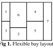
In this paper, we extend a mixed integer programming formulation for facility layout problem that was presented by Konak et al, [8]. They focus on flexible bay layout in which departments are located in vertical or horizontal columns (see Fig. 1). They consider single objective, minimizing departmental material handling cost. According to literature, there is no formulation for multi-objective facility layout problem. Our formulation involves both minimizing departmental material handling cost and maximizing closeness rating. To input closeness rating in the objective function, some constraints are necessary added to the previous model. We also modify our formulation to involve concurrent design layout and determine location of Input/Output (I/O) points with multi-objective approach. Paper is organized as follow: In section II mathematical model is presented, the approach of generating test problems is discussed in section III, computational results are stated in section IV, mathematical model to integrate determination of facility layout and locations of I/O points is presented in section and finally in
A Multi-Objective Formulation for Facility
Layout Problem
section VI, Conclusions are showed.
Fig 1. Flexible bay layout
II. MATHEMATICAL FORMULATION All notations and constraints of Konak et al. [8] formulation are used in our mathematical model, however to preserve vagueness, notations are stated here:
A. Parameter
Number of departments,
Width of the facility along the x-axis,
Length of the facility along the y-axis,
Maximum number of parallel bays,
Area requirement of department ,
Aspect ratio of department ,
Maximum permissible side length of department Minimum permissible side length of department
Amount of material flow between departments and ,
B. Variables
1,0, If department is assigned to bay ( Otherwise
-. /
1, If department is above department
in the same bay
0, Otherwise
-1 1,0, If bay ( is occupiedOtherwise
-4 Width (the length in the x-axis direction) of bay (,
5 Height (the length in the y-axis direction) of department ,
6 Height of department in bay (,
78, 859 Coordinates of the centered of department ,
: Distance between the centered of departments and
in the x-axis direction,
:5 Distance between the centered of departments and
in the y-axis direction.
In addition to these parameters and variables, we introduce some others as follow:
C. additional Parameter
: Adjacency ratio between departments
; Weighted of objective functions <0 = ; = 1>
D. additional variables
? /
1, If departments and have common
boundary
0, Otherwise
-7@;, @;
59 Coordinates of the north east corner of
department ,
7A84, A8459 Coordinatesof the south westcorner of department,
4,B Width (the length in the x-axis direction) of department in each bay (,
C8 The length of common boundary between departments and.
C8B Is equal to product of C8 and ?
E. Problem formulation
4B 4 D, ( <1>
Constraint (1) determines width of each department. It is linearized as follow:
4B = D, ( <1.1>
4B = 4F <1 G > D, ( <1.2>
4B I 4G <1 G > D, ( <1.3>
Proposition 1. Constraint (1) can be lineared as constraints (1.1) – (1.3).
Proof: If 1, then according to constraints (1.2) and (1.3) 4B is equal to 4. if 0, then according to constraint (1.1) 4B 0. If 4B K 0 then, constraint (1.1) causes to 1 and due to constraints (1.2) and (1.3) 4B is equal to 4.
L
L M8G 0.5 O 4 BP
G M8F 0.5 O 4B
PL L
= 71 G ?9 D Q <2>
R785G 0.5 59 G 785F 0.5 59R = 71 G ?9 D Q <3>
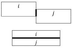
Constraint (2) and (3) are used to determine whether two departments have a common boundary. They state that if lower edge of a department is above upper edge of other department either in S-axis or ?-axis, these departments don’t have common boundary (see Figure 2.). They are linearized below:
M8G 0.5 O 4B
P
G M8F 0.5 O 4B
P
= 71 G ?9 D Q <2.1>
M8G 0.5 O 4B
P
G M8F 0.5 O 4B
P
= 71 G ?9 D Q <2.2>
785G 0.5 59 G 785F 0.5 59 = 71 G ?9 D Q <3.1>
785G 0.5
59 G 785F 0.5 59 = 71 G ?9 D Q <3.2> 1
3 6
7 4
[image:2.595.125.213.105.187.2]C8TM UV78 5F 0.5
5, 85F 0.5 59
GUS785G 0.5 5, 85G 0.5 59P
F
W X X
Y UV M8G 0.5 O 4 B , 8G 0.5 O
GUS M8F 0.5 O 4B
, 8F 0.5 O
(a)
(c)
Fig 2. (a) Lower edge of department is above upper edge of department in ?-axis, (b) Lower edge of department above upper edge of department in ?-axis, (c) L of department is above upper edge of department axis, (d) Lower edge of department is above upper edge of department in S-axis.
D
Constraint (4) calculates common boundary of each two departments if they have common boundary and if not it would be a negative number. The effect of this negative number can be eliminated easily as discussed later in describing the objective function. Figure 3 show
common boundaries between two departments.
Constraint (4) is linearized as follow:
@;5 8
5F 0.5 5
@; 8F O 4B
A845 85G 0.5 5
A84 8G 0.5 O 4B
Z = @;
Z = @;
Z5 = @; 5
Z5 = @; 5
[= 84
[= 84
Fig 3. Common boundary of two
9 9P
O 4BP
O 4B
P \ ] ] ^
(b)
(d)
is above upper edge of ower edge of department is , (c) Lower edge department in S -is above upper edge of
D Q (4)
Constraint (4) calculates common boundary of each two departments if they have common boundary and if not it effect of this negative as discussed later in Figure 3 shows types of common boundaries between two departments.
D <4.1>
D <4.2>
D <4.3>
D <4.4>
D Q <4.5> D Q <4.6>
D Q <4.7>
D Q <4.8>
D Q <4.9>
D Q <4.10>
[5 = 845 [5 = 845
C8 7ZG [9 F 7Z5G [
Min ; O O 7: F :59
e
G<1 G ;> O O
e
The objective function is given by
Objective function is sum weighted total of the departmental material handling costs and the maximum closeness rating.
C8 becomes a negative number it will cause the objective function to become worse. So
become zero automatically in
eliminated readily. Objective is linearized as follows:
C8B = < F >?
C8B = C8F < F >?
C8B I C8G < F >?
Min ; O O 7: F :59
e
G<1 G ;> O O C8B e
III. GENRATING TEST PROBL
Based on our knowledge, there is not any benchmark for multi-objective facility bay layout problem. So we have modified test problem in literature and customized it for our problem. We use test problem
single objective bay layout problem
we generate matrix of closeness rating between
Ye and Zhou [17] who quantify closeness ratings that are qualitative Relationships according to
We generate matrix of closeness rating matrix with random integer numbers in the range of
Also, we assume aspect ratio is four
departments, matrix of material handling cost and matrix with closeness rating of ten-sized test problem are
[image:3.595.305.552.86.196.2]Appendix.
Table 1. Relationship classification
Symbol Assigned number
f 5
Z 4
g 3
h 2
@ 1
i 0
After that, we generate test problems with sizing 5 to 9 with random selection of departments which are in ten
problem. Numbers of departments that are use test problems with sizing 5 to 9 are noted in
Common boundary of two departments
D Q <4.11> D Q <4.12>
[59 D Q <4.13>
9
O C8?
0 = ; = 1 <5>
The objective function is given by Equation (6). The is sum weighted total of the departmental material handling costs and the maximum closeness rating. If becomes a negative number it will cause the objective function to become worse. So ? which product in C8 become zero automatically in solving model and its effect is eliminated readily. Objective is linearized as follows:
D Q <5.1>
> D Q <5.2>
> D Q <5.3>
9 0 = ; = 1 <5.4>
GENRATING TEST PROBLEMS
Based on our knowledge, there is not any benchmark for objective facility bay layout problem. So we have test problem in literature and customized it for our We use test problem Van camp et al. [16] that is for single objective bay layout problem with ten departments, then we generate matrix of closeness rating between departments as quantify closeness ratings that are according to Table 1.
We generate matrix of closeness rating matrix with random in the range of j0,5k which has 20% density. Also, we assume aspect ratio is four< 4>. Areas of departments, matrix of material handling cost and matrix with sized test problem are seen in
1. Relationship classification
Assigned number Relationship
Absolutely necessary Especially important Important
Ordinary Unimportant Undesirable
[image:3.595.46.278.88.189.2] [image:3.595.46.263.262.367.2] [image:3.595.123.243.457.538.2]Table 2. Representation of test problems
Size Number of departments
5 1,2,6,7,9
6 1,4,6,7,8,9
7 1,3,4,5,6,8,9
8 2,3,4,5,6,7,8,10
9 2,3,4,5,6,7,8,9,10
10 1,2,3,4,5,6,7,8,9,10
IV. COMPUTATIONAL RESULTS
In flexible-bay layout problem, departments are located in vertical or horizontal columns and each department is located just in one bay. Number of bays is an integer number in the range of [1, n] and optimal number of bays is determined by solving the problem. In this paper, we use fixed-bay layout approach wherein number of bays is predetermined. We fixed the number of bays with considering 1 1 that ( is ranging from 1 to n. merely; we solve the mathematical model n times with different number of bays that is ranging from 1 to n instead of single running flexible-bay layout problem. We solve the problem for ; 0.1, 0.3, 0.5, 0.7, 0.9 to show the change of objective function in respect to the change of weighted of objective. We run mathematical model by use CPLEX10.1 software in a PC with 2.4 core Duo GHz CPU and 1GB RAM. The value of Objective function of each test problem is indicated in Table 3.
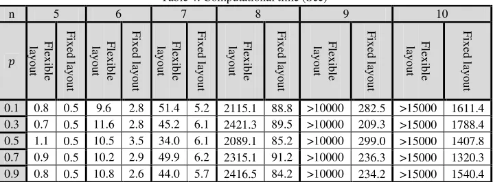
The summation of the computational time result of fixed-bay layout approach always is shorter than running problem with flexible bay as Table 4 illustrate. It is reasonable, because for some fixed-bay layout approach, there is no feasible solution. Also, in order to square shape of facility, having single bay is similar to having n bays with counterclockwise rotation (see fig 2.).
(a) (b)
Fig 3. (a) Single bay layout, (b) Layout with n bays.
We use a measure to compare computational result of fixed-bay layout approach versus to flexible-fixed-bay layout approach as follow:
mno <Time of qlexible‐bay‐Time of qixed‐bay>Time of qlexible bay u 100
Figure 4 shows that increasing size of problem causes to increase RPD.
V. BAY-LAYOUT PROBLEM CONSIDERING I/O POINTS In previous section, we assume I/O points are located in center of departments, whereas in industrial work, I/O points are located in perimeter of department specially, in intersections
points (see figure 6.)We assume departments have single I/O points.
1 4 8 2
9 7
3 6
5
Fig 6. Layout and I/O points (circle and arrow show I/O points )
To model bay layout considering I/O points we introduce some notation as follow:
<Sv, ?v> coordination of w th corner of department D, w Corner of each department are numbered as follow:
vB /
1, If wth point of department of U is I/O points of department w
S, otherwise
-:Svvy Distance between wth corner of department
to wBth corner of department in x-axis D, , w, wB
:?vvy Distance between wth corner of department
to wBth corner of department in y-axis D, , w, wB
zvB yvis an integer variable that is equal tozvB yu vB
[image:4.595.300.558.112.390.2] [image:4.595.302.558.407.764.2] [image:4.595.67.270.492.602.2]:S?vvy Is equal to RSvG SvyR u
|V ; O O O O O O 7RSvG SvyR
}
vT~ }
vyT~
T~
zT~ e
F R?vG ?vyR9vB zvB y
G<1 G ;> O O C8B e
(6)
We linearize constraint (7) as follow:
SvG Svy= :Svvy D Q , w, wB (6.1)
SvG Svy= :Svvy D Q , w, wB (6.2)
?vG ?vy= :?vvy D Q , w, wB (6.3)
1
2
3
4
5
1 2 3 4 5
0 25 50 75 100
4 5 6 7 8
R
P
D
(%
)
Number of departments
Fig 5. Effect of fixed bay respect to flexible bay on computational time
1 2
?vG ?vy= :?vvy D Q , w, wB (6.4)
zvB yv = vB D Q , w, wB, ;, U (6.5)
zvB yv = zvB y D Q , w, wB, ;, U (6.6)
zvB yv I zvB yF vB G 1 D Q , w, wB, ;, U (6.7)
O O vB
T~ }
vT~
1 D, w, U (6.8)
M8G 0.5 O 4B
P G Sv = <1 G vB > D, w, U (6.9)
Sv G M8F 0.5 O 4B
P = <1 G vB > D, w, U (6.10)
785G 0.5 59 G ?v = <1 G vB > D, w, U (6.11)
?v G 785F 0.5 59 = <1 G vB > D, w, U (6.12)
Product of an integer variable by continues variable can be linearize has proposition 1.
|V ; O O O O O O ::S?vvy
}
vT~ }
vyT~
T~
zT~ e
G<1 G ;> O O C8B e
; 0 = ; = 1
(6.13)
VI. CONCLUSIONS
In this paper, we extended a mixed integer programming formulation for facility layout problem that was presented by Konak et al. [8]. According to literature, there is no formulation for multi-objective facility layout problem. Our formulation involved both minimizing departmental material handling cost and maximizing closeness rating. Computational results show the effect of fixed-bay layout approach to flexible-bay layout approach. We also modified our formulation to involve concurrent design layout and determine location of I/O points with multi-objective approach. In spite of enormous complexity of layout problem considering I/O points, it can be used to find good lower bound for heuristic and metaheuristic approach. For future research we propose to develop a metaheuristic to consider concurrent determination of layout and locations of I/O points with multi-objective view.
APPENDIX
Material flow for the ten-department problem (van Camp et al.[16]).
Department 1 2 3 4 5 6 7 8 9 10
1 - 0 0 0 0 218 0 0 0 0
2 - 0 0 0 148 0 0 296 0
3 - 28 70 0 0 0 0 0
4 - 0 28 70 140 0 0
5 - 0 0 210 0 0
6 - 0 0 0 0
7 - 0 0 28
8 - 0 882
9 - 59.2
10 -
Aspect ratio <> 4
Departmental areas for the ten-department problem (van Camp et al.[16])
Department 1 2 3 4 5 6 7 8 9 10
Area 238 112 160 80 120 80 60 85 221 119
Closeness rating for the ten-department problem.
Department 1 2 3 4 5 6 7 8 9 10
1 - 3 0 0 0 0 4 0 5 0
2 - 0 0 0 2 0 4 1 1
3 - 0 5 0 5 0 0 1
4 - 0 0 3 0 1 2
5 - 0 0 1 0 5
6 - 0 0 0 2
7 - 0 0 0
8 - 2 0
9 - 0
10 -
References
[1] Aiello G, Enea M, Galante G, A multi-objective approach to facility layout problem by genetic search algorithm and Electre method, Robotics and Computer-Integrated Manufacturing, 22 (2006) 447-455.
[2] Arapoglu R. A, Norman B. A, Smith A. E, Locating input and output points in facilities design-A comparison of constructive, evolutionary, and exact methods, IEEE Transactions on Evolutionary Computation, 3 (2001) 192-203.
[3] Drira A, Pierreval H, Hajri-Gabouj S, Facility layout problems: A survey, Annual Reviews in Control, 31 (2007) 255-267.
[4] Farahani R. Z, Pourakbar M, Miandoabchi E, Developing exact and Tabu search algorithms for simultaneously determining AGV loop and P/D stations in single loop systems, International Journal of Production Research, 45 (2007) 5199-5222.
[5] Garey M. R, Johnson D. S, (1979). Computers and intractability: A guide to the theory of NP-completeness, WH Freeman, New York.
[6] Kim, J. G. and Goetschalckx, M., An integrated approach for the concurrent determination of the block layout and the input and output point locations based on the contour distance. International Journal of Production Research, 43 (10) (2005) 2027-2047.
[7] Konak A, Coit D. W, Smith A. E, Multi-objective optimization using genetic algorithms: A tutorial, Reliability Engineering and System Safety, 91 (2006) 992-1007.
[8] Konak A, Kulturel-Konak S, Norman B. A, Smith A. E, A new mixed integer programming formulation for facility layout design using flexible bays, Operations Research Letters, 34 (2006) 660-672.
[9] Kulturel-Konak S, Norman B. A, Smith A. E, Multi-objective tabu search using a multinomial probability mass function, European Journal of Operational Research, 169 (2006) 918-931.
Operations Research, 32 (2005) 879–899.
[11]Loiola E. M, de Abreu N. M. M, Boaventura-Netto P. O, Hahn P, Querido T, A survey for the quadratic assignment problem, European Journal of Operational Research, 176 (2007) 657-690.
[12]Singh S. P, Sharma R. R. K, A review of different approaches to the facility layout problems, International Journal of Advanced Manufacturing Technology, 30 (2006) 425-433.
[13]Sujono S, Lashkari R. S, A multi-objective model of operation allocation and material handling system selection in FMS design, International Journal of Production Economics, 105 (2007) 116-133.
[14]Suman B, Kumar P, A survey of simulated annealing as a tool for single and multi-objective optimization, Journal of the Operational Research Society, 57 (2006) 1143-1160.
[15]Tompkins J. A, Bozer Y. A, Tanchoco J. M. A, White J. A, Tanchoco J (2003). Facilities Planning, Wiley, New York.
[16]Van Camp D. J, Carter M. W, Vannelli A, A nonlinear optimization approach for solving facility layout problems, European Journal of Operational Research, 57 (1992) 174-189.
[image:6.595.308.539.110.203.2][17]Ye M, Zhou G, A local genetic approach to multi-objective, facility layout problems with fixed aisles, International Journal of Production Research, 45 (2007) 5243-5264.
Table 3. Objective function n
5 6 7 8 9 10
;
0.1 1184.6 312.5 460.1 1091.6 1584.1 2272.4
0.3 3744.4 1115.72 1722.2 3601.3 5179.4 7168.5
0.5 6304.3 1918.9 2984.2 6111.1 8769.8 12078.2
0.7 8864.1 2722.2 4246.2 8620.9 12360.2 16987.9
0.9 11424 3525.4 5508.2 11130.6 15950.6 21897.4
Table 4. Computational time (Sec)
n 5 6 7 8 9 10
;
F
le
x
ib
le
la
y
o
u
t
F
ix
ed
la
y
o
u
t
F
le
x
ib
le
la
y
o
u
t
F
ix
ed
la
y
o
u
t
F
le
x
ib
le
la
y
o
u
t
F
ix
ed
la
y
o
u
t
F
le
x
ib
le
la
y
o
u
t
F
ix
ed
la
y
o
u
t
F
le
x
ib
le
la
y
o
u
t
F
ix
ed
la
y
o
u
t
F
le
x
ib
le
la
y
o
u
t
F
ix
ed
la
y
o
u
t
[image:6.595.120.479.433.566.2]