Consensus Training for Consensus Decoding in Machine Translation

Consensus Training for Consensus Decoding in Machine Translation

Adam Pauls, John DeNero and Dan Klein Computer Science Division

University of California at Berkeley

{adpauls,denero,klein}@cs.berkeley.edu

Abstract

We propose a novel objective function for dis-criminatively tuning log-linear machine trans-lation models. Our objective explicitly op-timizes the BLEU score ofexpected n-gram counts, the same quantities that arise in forest-based consensus and minimum Bayes risk de-coding methods. Our continuous objective can be optimized using simple gradient as-cent. However, computing critical quantities in the gradient necessitates a novel dynamic program, which we also present here. As-suming BLEU as an evaluation measure, our objective function has two principle advan-tages over standard max BLEU tuning. First, it specifically optimizes model weights for downstream consensus decoding procedures. An unexpected second benefit is that it reduces overfitting, which can improve test set BLEU scores when using standard Viterbi decoding.

1 Introduction

Increasing evidence suggests that machine trans-lation decoders should not search for a single top scoring Viterbi derivation, but should instead choose a translation that is sensitive to the model’s entire predictive distribution. Several recent con-sensus decoding methods leverage compact repre-sentations of this distribution by choosing transla-tions according ton-gram posteriors and expected counts (Tromble et al., 2008; DeNero et al., 2009; Li et al., 2009; Kumar et al., 2009). This change in decoding objective suggests a complementary change intuningobjective, to one that optimizes expectedn-gram counts directly. The ubiquitous minimum error rate training (MERT) approach op-timizes Viterbi predictions, but does not explicitly boost the aggregated posterior probability of de-sirablen-grams (Och, 2003).

We therefore propose an alternative objective

function for parameter tuning, which we call con-sensus BLEU or CoBLEU, that is designed to maximize theexpected countsof then-grams that appear in reference translations. To maintain con-sistency across the translation pipeline, we for-mulate CoBLEU to share the functional form of BLEU used for evaluation. As a result, CoBLEU optimizes exactly the quantities that drive efficient consensus decoding techniques and precisely mir-rors the objective used for fast consensus decoding in DeNero et al. (2009).

CoBLEU is a continuous and (mostly) differ-entiable function that we optimize using gradient ascent. We show that this function and its gradient are efficiently computable over packed forests of translations generated by machine translation sys-tems. The gradient includes expectations of prod-uctsof features andn-gram counts, a quantity that has not appeared in previous work. We present a new dynamic program which allows the efficient computation of these quantities over translation forests. The resulting gradient ascent procedure does not require anyk-best approximations. Op-timizing over translation forests gives similar sta-bility benefits to recent work on lattice-based min-imum error rate training (Macherey et al., 2008) and large-margin training (Chiang et al., 2008).

We developed CoBLEU primarily to comple-ment consensus decoding, which it does; it pro-duces higher BLEU scores than coupling MERT with consensus decoding. However, we found an additional empirical benefit: CoBLEU is less prone to overfitting than MERT, even when using Viterbi decoding. In experiments, models trained to maximize tuning set BLEU using MERT con-sistently degraded in performance from tuning to test set, while CoBLEU-trained models general-ized more robustly. As a result, we found that op-timizing CoBLEU improved test set performance reliably using consensus decoding and occasion-ally using Viterbi decoding.

Once upon a rhyme

H1) Once on a rhyme

H3) Once upon a time H2) Once upon a rhyme

Il était une rime

(a) Tuning set sentence and translation

(a) Hypotheses ranked by !TM = !LM = 1

(a) Model score as a function of !LM Reference r:

Sentence f:

TM LM

-3 -7 0.67

-5 -6 0.24

-9 -3 0.09 Pr

(b) Objectives as functions of !LM (b) Computing Consensus Bigram Precision

-18 -12 -6 0

0 2

H3 H1

H2

Parameter: !LM

Model:

TM +

!LM

• LM

V

iterbi & Consensus Objectives

Parameter: !LM

Eθ[c(“Once upon”, d)|f] = 0.24 + 0.09 = 0.33

Eθ[c(“upon a”, d)|f] = 0.24 + 0.09 = 0.33

Eθ[c(“a rhyme”_! , d)|f] = 0.67 + 0.24 = 0.91

g

Eθ[c(g, d)|f] = 3[0.67 + 0.24 + 0.09] "

gmin_"{Eθ[c(g, d)|f], c(g, r)} gEθ[c(g, d)|f] =

0.33 + 0.33 + 0.91 3

Figure 1: (a) A simple hypothesis space of translations for a single sentence containing three alternatives, each with two features. The hypotheses are scored under a log-linear model with parametersθequal to the identity vector. (b) The expected counts of all bigrams that ap-pear in the computation of consensus bigram precision.

2 Consensus Objective Functions

Our proposed objective function maximizes n -gram precision by adapting the BLEU evaluation metric as a tuning objective (Papineni et al., 2002). To simplify exposition, we begin by adapting a simpler metric: bigram precision.

2.1 Bigram Precision Tuning

Let the tuning corpus consist of source sentences

F = f1. . . fm and human-generated references

R = r1. . . rm, one reference for each source sentence. Let ei be a translation of fi, and let

E =e1. . . embe a corpus of translations, one for each source sentence. A simple evaluation score forEis its bigram precision BP(R, E):

BP(R, E) = P_m

i=1

P

g2min{c(g2, ei), c(g2, ri)} P_m

i=1

P

g2c(g2, ei)

whereg2iterates over the set of bigrams in the tar-get language, andc(g2, e)is the count of bigram

g2in translatione. As in BLEU, we “clip” the bi-gram counts ofein the numerator using counts of bigrams in the reference sentence.

Modern machine translation systems are typi-cally tuned to maximize the evaluation score of

Viterbi derivations1_{under a log-linear model with} parametersθ. Letd∗

θ(fi) = arg maxdPθ(d|fi) be the highest scoring derivationdoffi. For a system employing Viterbi decoding and evaluated by bi-gram precision, we would want to selectθto max-imize MaxBP(R, F, θ):

P_m

i=1P_Pg2min{c(g2, dθ∗(fi)), c(g2, ri)}

m

i=1Pg2c(g2, d∗θ(fi))

On the other hand, for a system that uses ex-pected bigram counts for decoding, we would pre-fer to chooseθsuch that expected bigram counts match bigrams in the reference sentence. To this end, we can evaluate an entire posterior distri-bution over derivations by computing the same clipped precision for expected bigram counts us-ing CoBP(R, F, θ):

P_m

i=1

P

g2min{Eθ[c(g2, d)|fi], c(g2, ri)} P_m

i=1

P

g2Eθ[c(g2, d)|fi]

(1)

where

Eθ[c(g2, d)|fi] =

X

d

Pθ(d|fi)c(g2, d)

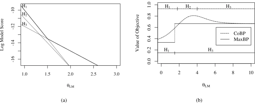
is the expected count of bigram g2 in all deriva-tions d of fi. We define the precise parametric form ofPθ(d|fi)in Section 3. Figure 1 shows pro-posed translations for a single sentence along with the bigram expectations needed to compute CoBP. Equation 1 constitutes an objective function for tuning the parameters of a machine translation model. Figure 2 contrasts the properties of CoBP and MaxBP as tuning objectives, using the simple example from Figure 1.

Consensus bigram precision is an instance of a general recipe for convertingn-gram based eval-uation metrics into consensus objective functions for model tuning. For the remainder of this pa-per, we focus on consensus BLEU. However, the techniques herein, including the optimization ap-proach of Section 3, are applicable to many differ-entiable functions of expectedn-gram counts.

1_{Byderivation, we mean a translation of a foreign}

1.0 1.5 2.0 2.5 3.0

-16

-14

-12

-10

θLM

Log Model Score

H1 H2

H3

(a)

0 2 4 6 8 10

0.0

0.2

0.4

0.6

0.8

1.0

θLM

Value of Objective

CoBP MaxBP

H1 H3

H1 H2 H3

(b)

Figure 2: These plots illustrate two properties of the objectivesmax bigram precision(MaxBP) and consensus bigram precision(CoBP) on the simple example from Figure 1. (a) MaxBP is only sensitive to the convex hull (the solid line) of model scores. When varying the single parameterθLM, it entirely disregards the correct translation H2becauseH2never attains a maximal model score. (b) A plot of both objectives shows their differing characteris-tics. The horizontal segmented line at the top of the plot indicates the range over which consensus decoding would select each hypothesis, while the segmented line at the bottom indicates the same for Viterbi decoding. MaxBP is only sensitive to the single point of discontinuity betweenH1andH3, and disregardsH2entirely. CoBP peaks when the distribution most heavily favorsH2while suppressingH1. ThoughH2never has a maximal model score, ifθLMis in the indicated range, consensus decoding would selectH2, the desired translation.

2.2 CoBLEU

The logarithm of the single-reference2_BLEU met-ric (Papineni et al., 2002) has the following form:

lnBLEU(R, E) = 1−P_m |R|

i=1

P

g1c(g1, ei) !

−

+1₄

4

X

n=1

ln P_m

i=1

P

gnmin{c(gn, ei), c(gn, ri)} P_m

i=1

P

gnc(gn, ei)

Above,|R|denotes the number of words in the reference corpus. The notation(·)− is shorthand formin(·,0). In the inner sums,gniterates over all n-grams of ordern. In order to adapt BLEU to be a consensus tuning objective, we follow the recipe of Section 2.1: we replacen-gram counts from a candidate translation with expectedn-gram counts under the model.

CoBLEU(R, F, θ)= 1−P_m |R|

i=1

P

g1Eθ[c(g1, d)|fi] !

−

+1₄X4 n=1

ln P_m

i=1

P

gnmin{Eθ[c(gn, d)|fi], c(gn, ri)} P_m

i=1

P

gnEθ[c(gn, d)|fi]

The brevity penalty term in BLEU is calculated using the expected length of the corpus, which

2_{Throughout this paper, we use only a single reference,}

but our objective readily extends to multiple references.

equals the sum of all expected unigram counts. We call this objective functionconsensus BLEU, or CoBLEU for short.

3 Optimizing CoBLEU

Unlike the more common MaxBLEU tuning ob-jective optimized by MERT, CoBLEU is con-tinuous. For distributions Pθ(d|fi) that factor over synchronous grammar rules andn-grams, we show below that it is also analytically differen-tiable, permitting a straightforward gradient ascent optimization procedure.3 _{In order to perform} gra-dient ascent, we require methods for efficiently computing the gradient of the objective function for a given parameter settingθ. Once we have the gradient, we can perform an update at iterationt

of the form

θ(t+1) ←θ(t)+ηt∇θCoBLEU(R, F, θ(t))

whereηtis an adaptive step size.4

3_{Technically, CoBLEU is non-differentiable at some}

points because ofclipping. At these points, we must com-pute a gradient, and so our optimization is formally sub-gradient ascent. See the Appendix for details.

4_{After each successful step, we grow the step size by a}

head(h)

tail(h) u=OnceSrhyme

v1=OnceRBOnce v2=uponINupon v3=aNPrhyme c(“Once upon”, h)

c(“upon a”, h)

= 1 = 1

!2(h) = 2

Figure 3: A hyperedgeh represents a “rule” used in syntactic machine translation.tail(h)refers to the “chil-dren” of the rule, whilehead(h)refers to the “head” or “parent”. A forest of translations is built by combining the nodesviusinghto form a new nodeu=head(h).

Each forest node consists of a grammar symbol and tar-get language boundary words used to trackn-grams. In the above, we keep one boundary word for each node, which allows us to track bigrams.

In this section, we develop an analytical expres-sion for the gradient of CoBLEU, then discuss how to efficiently compute the value of the objec-tive function and gradient.

3.1 Translation Model Form

We first assume the general hypergraph setting of Huang and Chiang (2007), namely, that deriva-tions under our translation model form a hyper-graph. This framework allows us to speak about both phrase-based and syntax-based translation in a unified framework.

We define a probability distribution over deriva-tionsdviaθas:

Pθ(d|fi) = _Z(fw(d) i)

with

Z(fi) =

X

d0

w(d0₎

wherew(d) = exp(θ>_{Φ(d, fi))is the weight of a} derivation andΦ(d, fi)is a featurized representa-tion of the derivarepresenta-tiondoffi. We further assume that these features decompose overhyperedgesin the hypergraph, like the one in Figure 3. That is,

Φ(d, fi) =Ph∈dΦ(h, fi).

In this setting, we can analytically compute the gradient of CoBLEU. We provide a sketch of the derivation of this gradient in the Appendix. In computing this gradient, we must calculate the

fol-lowing expectations:

Eθ[c(φk, d)|fi] (2)

Eθ[`n(d)|fi] (3)

Eθ[c(φk, d)·`n(d)|fi] (4)

where`n(d) = Pgnc(gn, d)is the sum of alln -grams on derivationd(its “length”). The first ex-pectation is an expected count of thekth feature

φkover all derivations offi. The second is an ex-pected length, the total exex-pected count of all n -grams in derivations of fi. We call the final ex-pectation an expectedproduct of counts. We now present the computation of each of these expecta-tions in turn.

3.2 Computing Feature Expectations

The expected feature countsEθ[c(φk, d)|fi]can be written as

Eθ[c(φk, d)|fi] =

X

d

Pθ(d|fi)c(φk, d)

= X

h

Pθ(h|fi)c(φk, h)

We can justify the second step since fea-ture counts are local to hyperedges, i.e.

c(φk, d) = Ph∈dc(φk, h). The posterior probability Pθ(h|fi) can be efficiently computed with inside-outside scores. Let I(u)and O(u) be the standard inside and outside scores for a node

uin the forest.5

Pθ(h|fi) = _Z(f1 ₎ w(h)O(head(h))

Y

v∈tail(h) I(v)

where w(h) is the weight of hyperedge h, given by exp(θ>_{Φ(h)), andZ(f) = I(root) is the} in-side score of the root of the forest. Computing these inside-outside quantities takes time linear in the number of hyperedges in the forest.

3.3 Computingn-gram Expectations

We can compute the expectations of any specific

n-grams, or of totaln-gram counts`, in the same way as feature expectations, provided that target-siden-grams are also localized to hyperedges (e.g. consider ` to be a feature of a hyperedge whose value is the number of n-grams on h). If the nodes in our forests are annotated with target-side

boundary words as in Figure 3, then this will be the case. Note that this is the same approach used by decoders which integrate a target language model (e.g. Chiang (2007)). Other work has computed

n-gram expectations in the same way (DeNero et al., 2009; Li et al., 2009).

3.4 Computing Expectations of Products of Counts

While the previous two expectations can be com-puted using techniques known in the literature, the expected product of countsEθ[c(φk, d)·`n(d)|fi] is a novel quantity. Fortunately, an efficient dy-namic program exists for computing this expec-tation as well. We present this dynamic program here as one of the contributions of this paper, though we omit a full derivation due to space re-strictions.

To see why this expectation cannot be computed in the same way as the expected feature orn-gram counts, we expand the definition of the expectation above to get

X

d

Pθ(d|fi) [c(φk, d)`n(d)]

Unlike feature andn-gram counts, the product of counts in brackets above does not decompose over hyperedges, at least not in an obvious way. We can, however, still decompose the feature counts

c(φk, d) over hyperedges. After this decomposi-tion and a little re-arranging, we get

= X

h

c(φk, h)

X

d:h∈d

Pθ(d|fi)`n(d)

= _Z(1_f i)

X

h

c(φk, h)

" X

d:h∈d

w(d)`n(d)

#

= _Z(1_f i)

X

h

c(φk, h)ˆDnθ(h|fi)

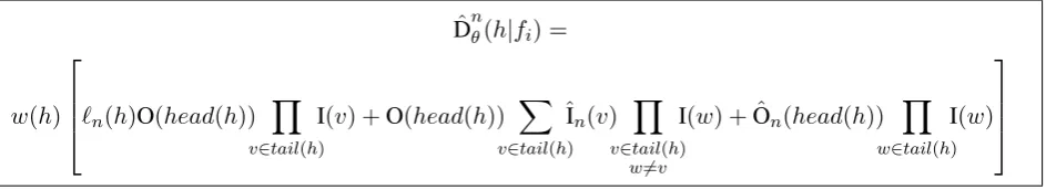
The quantityDˆn_θ(h|fi) =Pd:h∈dw(d)`n(d)is the sum of the weight-length products of all deriva-tions d containing hyperedge h. In the same way that Pθ(h|fi) can be efficiently computed from inside and outside probabilities, this quan-tityDˆn_θ(h|fi)can be efficiently computed with two new inside and outside quantities, which we call

ˆ_In(u)andOˆ_{n(u). We provide recursions for these}

quantities in Figure 4. Like the standard inside and outside computations, these recursions run in time linear in the number of hyperedges in the forest.

While a full exposition of the algorithm is not possible in the available space, we give some brief

intuition behind this dynamic program. We first defineˆIn(u):

ˆ_{In(u) =}X

du

w(du)`n(d)

wheredu is a derivation rooted at nodeu. This is a sum of weight-length products similar toD. Toˆ give a recurrence forˆI, we rewrite it:

ˆ_{In(u) =}X

du

X

h∈du

[w(du)`n(h)]

Here, we have broken up the total value of`n(d) across hyperedges in d. The bracketed quantity is a score of amarked derivationpair(d, h)where the edgehis some specific element ofd. The score of a marked derivation includes the weight of the derivation and the factor`n(h)for the marked hy-peredge.

This sum over marked derivations gives the in-side recurrence in Figure 4 by the following de-composition. ForˆIn(u) to sum over all marked derivation pairs rooted atu, we must consider two cases. First, the marked hyperedge could be at the root, in which case we must choose child deriva-tions from regular inside scores and multiply in the local`n, giving the first summand ofˆIn(u). Alter-natively, the marked hyperedge is in exactly one of the children; for each possibility we recursively choose a marked derivation for one child, while the other children choose regular derivations. The second summand of ˆIn(u) compactly expresses a sum over instances of this case. Oˆn(u) de-composes similarly: the marked hyperedge could be local (first summand), under a sibling (second summand), or higher in the tree (third summand).

Once we have these new inside-outside quanti-ties, we can computeD as in Figure 5. This com-ˆ bination states that marked derivations containing

hare either marked ath, belowh, or aboveh. As a final detail, computing the gradient ∇Cnclip(θ) (see the Appendix) involves a clipped version of the expected product of counts, for which a clippedDˆ is required. This quantity can be computed with the same dynamic program with a slight modification. In Figure 4, we show the dif-ference as a choice point when computing`n(h).

3.5 Implementation Details

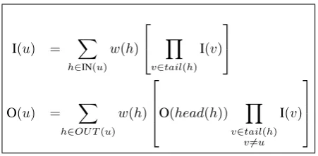
ˆ_{In(u) =}X h∈IN(u)

w(h) 

_`n(h) Y

v∈tail(h)

I(v) + X v∈tail(h)

ˆ_In(v)Y w6=v

I(w)  

ˆ

On(u) =

X

h∈OUT(u)

w(h)     

`n(h)O(head(h)) Y

v∈tail(h)

v6=u

I(v) + O(head(h))X v∈tail(h)

v6=u

ˆ_In(v)Y w∈tail(h)

w6=v w6=u

I(w) + ˆOn(head(h))

Y

w∈tail(h)

w6=u

I(w)      

`n(h) =

(P

gnc(gn, h) computing unclipped counts P

gnc(gn, h)1[Eθ[c(gn, d)]≤c(gn, ri)] computing clipped counts

Figure 4: Inside and Outside recursions forˆIn(u) andOˆn(u). IN(u) and OUT(u) refer to the incoming and

outgoing hyperedges ofu, respectively. I(·)and O(·)refer to standard inside and outside quantities, defined in Appendix Figure 7. We initialize withˆIn(u) = 0for all terminal forest nodesuandOˆn(root) = 0for the root

node.`n(h)computes the sum of alln-grams of ordernon a hyperedgeh.

ˆ

Dn_θ(h|fi) =

w(h)

  

`n(h)O(head(h))

Y

v∈tail(h)

I(v) +O(head(h)) X

v∈tail(h)

ˆ_In(v) Y

v∈tail(h) w6=v

I(w) + ˆOn(head(h)) Y

w∈tail(h) I(w)

   

Figure 5: Calculation ofDˆn_θ(h|fi)afterˆIn(u)andOˆn(u)have been computed.

number of hyperedges is very large, however, be-cause we must trackn-gram contexts in the nodes, just as we would in an integrated language model decoder. These contexts are required both to cor-rectly compute the model score of derivations and to compute clippedn-gram counts. To speed our computations, we use the cube pruning method of Huang and Chiang (2007) with a fixed beam size. For regularization, we added an L2 penalty on the size of θ to the CoBLEU objective, a simple addition for gradient ascent. We did not find that our performance varied very much for moderate levels of regularization.

3.6 Related Work

The calculation of expected counts can be for-mulated using the expectation semiring frame-work of Eisner (2002), though that frame-work does not show how to compute expected products of counts which are needed for our gradient calcu-lations. Concurrently with this work, Li and Eis-ner (2009) have geEis-neralized EisEis-ner (2002) to com-pute expected products of counts on translation forests. The training algorithm of Kakade et al. (2002) makes use of a dynamic program similar to

ours, though specialized to the case of sequence models.

4 Consensus Decoding

Once model parameters θ are learned, we must select an appropriate decoding objective. Sev-eral new decoding approaches have been proposed recently that leverage some notion of consensus over the many weighted derivations in a transla-tion forest. In this paper, we adopt the fast consen-sus decoding procedure of DeNero et al. (2009), which directly complements CoBLEU tuning. For a source sentence f, we first build a translation forest, then compute the expected count of each

n-gram in the translation of f under the model. We extract ak-best list from the forest, then select the translation that yields the highest BLEU score relative to the forest’s expected n-gram counts. Specifically, let BLEU(e;r) compute the simi-larity of a sentence e to a reference r based on the n-gram counts of each. When training with CoBLEU, we replaceewith expected counts and maximizeθ. In consensus decoding, we replacer

with expected counts and maximizee.

cedures would similarly benefit from a tuning pro-cedure that aggregates over derivations. For in-stance, Blunsom and Osborne (2008) select the translation sentence with highest posterior proba-bility under the model, summing over derivations. Li et al. (2009) propose a variational approxima-tion maximizing sentence probability that decom-poses over n-grams. Tromble et al. (2008) min-imize risk under a loss function based on the lin-ear Taylor approximation to BLEU, which decom-poses overn-gram posterior probabilities.

5 Experiments

We compared CoBLEU training with an imple-mentation of minimum error rate training on two language pairs.

5.1 Model

Our optimization procedure is in principle tractable for any syntactic translation system. For simplicity, we evaluate the objective using an In-version Transduction Grammar (ITG) (Wu, 1997) that emits phrases as terminal productions, as in (Cherry and Lin, 2007). Phrasal ITG models have been shown to perform comparably to the state-of-the art phrase-based system Moses (Koehn et al., 2007) when using the same phrase table (Petrov et al., 2008).

We extract a phrase table using the Moses pipeline, based on Model 4 word alignments gen-erated from GIZA++ (Och and Ney, 2003). Our fi-nal ITG grammar includes the five standard Moses features, ann-gram language model, a length ture that counts the number of target words, a fea-ture that counts the number of monotonic ITG rewrites, and a feature that counts the number of inverted ITG rewrites.

5.2 Data

We extracted phrase tables from the Spanish-English and French-Spanish-English sections of the Eu-roparl corpus, which include approximately 8.5 million words of bitext for each of the language pairs (Koehn, 2002). We used a trigram lan-guage model trained on the entire corpus of En-glish parliamentary proceedings provided with the Europarl distribution and generated according to the ACL 2008 SMT shared task specifications.6 For tuning, we used all sentences from the 2007 SMT shared task up to length 25 (880 sentences

6_{Seehttp://www.statmt.org/wmt08for details.}

2 4 6 8 10

0.0

0.2

0.4

0.6

0.8

1.0

Iterations

Fraction of Value at Convergence

CoBLEU MERT

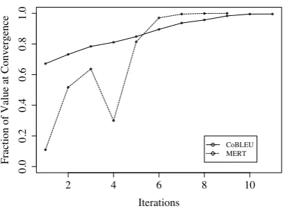
Figure 6: Trajectories of MERT and CoBLEU dur-ing optimization show that MERT is initially unstable, while CoBLEU training follows a smooth path to con-vergence. Because these two training procedures op-timize different functions, we have normalized each trajectory by the final objective value at convergence. Therefore, the absolute values of this plot do not re-flect the performance of either objective, but rather the smoothness with which the final objective is ap-proached. The rates of convergence shown in this plot are not directly comparable. Each iteration for MERT above includes 10 iterations of coordinate ascent, fol-lowed by a decoding pass through the training set. Each iteration of CoBLEU training involves only one gradi-ent step.

for Spanish and 923 for French), and we tested on the subset of the first 1000 development set sen-tences which had length at most 25 words (447 sentences for Spanish and 512 for French).

5.3 Tuning Optimization

We compared two techniques for tuning the nine log-linear model parameters of our ITG grammar. We maximized CoBLEU using gradient ascent, as described above. As a baseline, we maximized BLEU of the Viterbi translation derivations using minimum error rate training. To improve opti-mization stability, MERT used a cumulativek-best list that included all translations generated during the tuning process.

Consensus Decoding

Spanish Tune Test ∆ Br. MERT 32.5 30.2 -2.3 0.992 CoBLEU 31.4 30.4 -1.0 0.992 MERT→CoBLEU 31.7 30.8 -0.9 0.992

French

Tune Test ∆ Br. MERT 32.5 31.1* -1.4 0.972 CoBLEU 31.9 30.9 -1.0 0.954 MERT→CoBLEU 32.4 31.2* -0.8 0.953

Table 1: Performance measured by BLEU using a con-sensus decoding method over translation forests shows an improvement over MERT when using CoBLEU training. The first two conditions were initialized by 0 vectors. The third condition was initialized by the final parameters of MERT training. Br. indicates the brevity penalty on the test set. The * indicates differ-ences which are not statistically significant.

smoothly to its final objective because the forests do not change substantially between iterations, de-spite the pruning needed to trackn-grams. Similar stability benefits have been observed for lattice-based MERT (Macherey et al., 2008).

5.4 Results

We performed experiments from both French and Spanish into English under three conditions. In the first two, we initialized both MERT and CoBLEU training uniformly with zero weights and trained until convergence. In the third condition, we ini-tialized CoBLEU with the final parameters from MERT training, denoted MERT→CoBLEU in the results tables. We evaluated each of these condi-tions on both the tuning and test sets using the con-sensus decoding method of DeNero et al. (2009). The results appear in Table 1.

In Spanish-English, CoBLEU slightly outper-formed MERT under the same initialization, while the opposite pattern appears for French-English. The best test set performance in both language pairs was the third condition, in which CoBLEU training was initialized with MERT. This con-dition also gave the highest CoBLEU objective value. This pattern indicates that CoBLEU is a useful objective for translation with consensus de-coding, but that the gradient ascent optimization is getting stuck in local maxima during tuning. This issue can likely be addressed with annealing, as described in (Smith and Eisner, 2006).

Interestingly, the brevity penatly results in French indicate that, even though CoBLEU did

Viterbi Decoding

Spanish Tune Test ∆

MERT 32.5 30.2 -2.3

MERT→CoBLEU 30.5 30.9 +0.4

French Tune Test ∆

MERT 32.0 31.0 -1.0

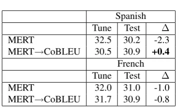
MERT→CoBLEU 31.7 30.9 -0.8 Table 2: Performance measured by BLEU usingViterbi

decoding indicates that CoBLEU is less prone to over-fitting than MERT.

not outperform MERT in a statistically significant way, CoBLEU tends to find shorter sentences with highern-gram precision than MERT.

Table 1 displays a second benefit of CoBLEU training: compared to MERT training, CoBLEU performance degrades less from tuning to test set. In Spanish, initializing with MERT-trained weights and then training with CoBLEU actually decreases BLEU on the tuning set by 0.8 points. However, this drop in tuning performance comes with a corresponding increase of 0.6 on the test set, relative to MERT training. We see the same pattern in French, albeit to a smaller degree.

While CoBLEU ought to outperform MERT us-ing consensus decodus-ing, we expected that MERT would give better performance under Viterbi de-coding. Surprisingly, we found that CoBLEU training actually outperformed MERT in Spanish-English and performed equally well in French-English. Table 2 shows the results. In these ex-periments, we again see that CoBLEU overfit the training set to a lesser degree than MERT, as evi-denced by a smaller drop in performance from tun-ing to test set. In fact, test set performance actually improved for Spanish-English CoBLEU training while dropping by 2.3 BLEU for MERT.

6 Conclusion

Appendix: The Gradient of CoBLEU

We would like to compute the gradient of

1−P_m |R|

i=1

P

g1Eθ[c(g1, d)|fi] !

−

+1₄

4

X

n=1

ln P_m

i=1

P

gnmin{Eθ[c(gn, d)|fi], c(gn, ri)} P_m

i=1

P

gnEθ[c(gn, d)|fi] To simplify notation, we introduce the functions

Cn(θ) = m

X

i=1

X

gn

Eθ[c(gn, e)|fi]

Cclip n (θ) =

m

X

i=1

X

gn

min{Eθ[c(gn, d)|fi], c(r, gn)}

Cn(θ)represents the sum of the expected counts of all n-grams or order n in all translations of the source corpusF, whileCnclip(θ)represents the sum of the same expected counts, but clipped with reference countsc(gn, ri).

With this notation, we can write our objective function CoBLEU(R, F, θ)in three terms:

1− _C|R|

1(θ)

−

+1₄

4

X

n=1

lnC_nclip(θ)− 1₄ 4

X

n=1

lnCn(θ)

We first state an identity: X

gn ∂

∂θkEθ[c(gn, d)|fi] =

Eθ[c(φk, d)·`n(d)|fi]

−Eθ[`n(d)|fi]·Eθ[c(φk, d)|fi]

which can be derived by expanding the expectation on the left-hand side

X

gn X

d ∂

∂θkPθ(d|fi)c(gn, d)

and substituting

∂

∂θkPθ(d|fi) =

Pθ(d|fi)c(φk, d)−Pθ(d|fi)

X

d0

Pθ(d0|fi)c(φk, d0)

Using this identity and some basic calculus, the gradient∇Cn(θ)is

m

X

i=1

Eθ[c(φk, d)·`n(d)|fi]−Cn(θ)Eθ[c(φk, d)|fi]

I(u) = X h∈IN(u)

w(h) 

 Y

v∈tail(h) I(v)

 

O(u) = X h∈OUT(u)

w(h)   

O(head(h)) Y

v∈tail(h)

v6=u

I(v)    

Figure 7: Standard Inside-Outside recursions which compute I(u)and O(u). IN(u)and OUT(u)refer to the incoming and outgoing hyperedges ofu, respectively. We initialize with I(u) = 1for all terminal forest nodes

uand O(root) = 1for the root node. These quantities are referenced in Figure 4.

and the gradient∇Cnclip(θ)is given by m

X

i=1

X

gn "

Eθ[c(gn, d)·c(φk, d)|fi]

·1hEθ[c(gn, d)|fi]≤c(gn, ri)

i#

−Cclip

n (θ)Eθ[c(φk, d) +fi]

where1denotes an indicator function. At the top level, the gradient of the first term (the brevity penalty) is

|R|∇C1(θ)

C1(θ)2 1

h

C1(θ)≤ |R|

i

The gradient of the second term is

1 4

4

X

n=1

∇Cnclip(θ)

Cnclip(θ)

and the gradient of the third term is

−1₄

4

X

n=1

∇Cn(θ)

Cn(θ)

References

Phil Blunsom and Miles Osborne. 2008. Probabilistic inference for machine translation. In Proceedings of the Conference on Emprical Methods for Natural Language Processing.

Colin Cherry and Dekang Lin. 2007. Inversion trans-duction grammar for joint phrasal translation mod-eling. InThe Annual Conference of the North Amer-ican Chapter of the Association for Computational Linguistics Workshop on Syntax and Structure in Statistical Translation.

David Chiang, Yuval Marton, and Philip Resnik. 2008. Online large-margin training of syntactic and struc-tural translation features. InThe Conference on Em-pirical Methods in Natural Language Processing. David Chiang. 2007. Hierarchical phrase-based

trans-lation. Computational Linguistics.

John DeNero, David Chiang, and Kevin Knight. 2009. Fast consensus decoding over translation forests. In

The Annual Conference of the Association for Com-putational Linguistics.

Jason Eisner. 2002. Parameter estimation for prob-abilistic finite-state transducers. In Proceedings of the 40th Annual Meeting on Association for Compu-tational Linguistics.

Liang Huang and David Chiang. 2007. Forest rescor-ing: Faster decoding with integrated language mod-els. InThe Annual Conference of the Association for Computational Linguistics.

Sham Kakade, Yee Whye Teh, and Sam T. Roweis. 2002. An alternate objective function for markovian fields. InProceedings of ICML.

Philipp Koehn, Hieu Hoang, Alexandra Birch, Chris Callison-Burch, Marcello Federico, Nicola Bertoldi, Brooke Cowan, Wade Shen, Christine Moran, Richard Zens, Chris Dyer, Ondrej Bojar, Alexandra Constantin, and Evan Herbst. 2007. Moses: Open source toolkit for statistical machine translation. In

The Annual Conference of the Association for Com-putational Linguistics.

Philipp Koehn. 2002. Europarl: A multilingual corpus for evaluation of machine translation.

Shankar Kumar, Wolfgang Macherey, Chris Dyer, and Franz Och. 2009. Efficient minimum error rate training and minimum Bayes-risk decoding for translation hypergraphs and lattices. InThe Annual Conference of the Association for Computational Linguistics.

Zhifei Li and Jason Eisner. 2009. First- and second-order expectation semirings with applications to minimum-risk training on translation forests. In

Proceedings of the 2009 Conference on Empirical Methods in Natural Language Processing.

Zhifei Li, Jason Eisner, and Sanjeev Khudanpur. 2009. Variational decoding for statistical machine transla-tion. In The Annual Conference of the Association for Computational Linguistics.

W. Macherey, F. Och, I. Thayer, and J. Uszkoreit. 2008. Lattice-based minimum error rate training for statistical machine translation. InIn Proceedings of Empirical Methods in Natural Language Process-ing.

Franz Josef Och and Hermann Ney. 2003. A sys-tematic comparison of various statistical alignment models. Computational Linguistics, 29:19–51. Franz Josef Och. 2003. Minimum error rate training

in statistical machine translation. InProceedings of the 41st Annual Meeting on Association for Compu-tational Linguistics (ACL), pages 160–167, Morris-town, NJ, USA. Association for Computational Lin-guistics.

Kishore Papineni, Salim Roukos, Todd Ward, and Wei-Jing Zhu. 2002. BLEU: A method for automatic evaluation of machine translation. In The Annual Conference of the Association for Computational Linguistics.

Slav Petrov, Aria Haghighi, and Dan Klein. 2008. Coarse-to-fine syntactic machine translation us-ing language projections. In Proceedings of the 2008 Conference on Empirical Methods in Nat-ural Language Processing, pages 108–116, Hon-olulu, Hawaii, October. Association for Computa-tional Linguistics.

David Smith and Jason Eisner. 2006. Minimum risk annealing for training log-linear models. InIn Pro-ceedings of the Association for Computational Lin-guistics.

Roy Tromble, Shankar Kumar, Franz Och, and Wolf-gang Macherey. 2008. Lattice minimum Bayes-risk decoding for statistical machine translation. InThe Conference on Empirical Methods in Natural Lan-guage Processing.

Dekai Wu. 1997. Stochastic inversion transduction grammars and bilingual parsing of parallel corpora.