Simple Singular Perturbation Problems with Turning Points

(1)

ISSN Online: 2327-4379 ISSN Print: 2327-4352

DOI: 10.4236/jamp.2019.712208 Dec. 6, 2019 2979 Journal of Applied Mathematics and Physics

Simple Singular Perturbation Problems with

Turning Points

Na Wang

Department of Applied Mathematics, Shanghai Institute of Technology, Shanghai, China

Abstract

The paper considers the asymptotic solution of two-point boundary value problems

ε

y′′+A x y

( )

′=0, 0≤ ≤x 1_{, when}0<

ε

_1_,_A₍_x_{) is smooth with}

isolated zeros, y

( )

0 =0_and y

( )

1 1= _{. By using perturbation method, the}

limit asymptotic solutions of various cases are obtained. We provide a reliable and direct method for solving similar problems. The limiting solutions are constants in this paper, except in narrow boundary and interior layers of nonuniform convergence. These provide simple examples of boundary layer resonance.

Keywords

Singular Perturbations, Asymptotic Methods, Boundary Value Problems, Turning Points, Boundary and Interior Layers, Boundary Layer Resonance

1. Introduction

A typical turning point problem consists of the linear differential equation

0,

y xy ny

ε ′′− ′+ = ₍₁₎

for a nonnegative integer n on − ≤ ≤1 x 1_{with prescribed boundary values}

( )

1

y ± _{and a small positive parameter}ε_,_i.e._, 0<

ε

1. Limiting solutions, away from narrow so-called boundary and interior shock layers of rapid change, take the form

( )

0 n

Y x =x C₍₂₎

as

ε

→0 for constants C, so satisfy the limiting reduced equation

0 0.

xY′ =nY ₍₃₎

Determining constants C and the location of layers is a nontrivial task, the

How to cite this paper: Wang, N. (2019) Simple Singular Perturbation Problems with Turning Points. Journal of Applied Mathematics and Physics, 7, 2979-2989. https://doi.org/10.4236/jamp.2019.712208

Received: November 26, 2019 Accepted: December 3, 2019 Published: December 6, 2019

(2)

DOI: 10.4236/jamp.2019.712208 2980 Journal of Applied Mathematics and Physics

subject of boundary layer resonance [1]. It involves detailed asymptotic analysis and often uses special functions. The classical techniques of matched asymptotic expansions [2][3] and the boundary function method of Vasil’eva et al.[4] may break down, though the newer composite asymptotic expansions [5] seem to ap-ply. Many experts have studied such problems over the last fifty years [6][7][8]

for surveys. An important application to stochastic differential equations in de-scribed in the 2017 SIAM von Neumann lecture by Matkowsky [9]. Computing solutions to such problems remains a challenge, although Trefethen et al.[10]

succeed for some examples using the program Chebfun.

A simple, but still rich, the related problem concerns the asymptotic solution of the two-point problem [11]

( )

0, 0 1,

y A x y x

ε

′′+ ′= ≤ ≤ (4)

with the special boundary values

( )

0 0 and 1 1

( )

y = y = (5)

and a smooth coefficient A x

( )

. Its unique exact solution is

( )

( ) ( ) 0 0 1 _d 0 1 _d 1 0 e d , . e d s s

A t t x

A t t

s y x s ε ε ε − − ∫ ∫ =

∫

(6) Since

( )

( ) ( ) 0 0 1 _d 1 _d 1 0 e , 0, e d x s A t t

A t t y x s ε ε ε − − ∫ ∫

′ = >

∫

(7)

the solution y will increase monotonically with x. The asymptotic value of

( )

0 , d

x

I s

ε

s

∫

in (6) is the area under the curve

( )

_, _e 10sA t t( )d

I s

_ε

_≡ −ε∫ ₍₈₎

for

ε

→0_{. Sophisticated techniques to obtain the asymptotic evaluation of}

in-tegrals can be found in Olver [12], Wong [13] and elsewhere. Simple arguments often provide the limiting ratio (6), often after rescaling I.

The variety of limiting behaviors to singularly perturbed linear two-point boundary value problems with turning points has not been clearly described. The first papers by Pearson in 1968 stressed a numerical approach. In the inter-vening fifty years, software has improved tremendously, though finding the li-miting solution is extremely ill-conditioned as Trefethen recently observed. Due to the serious instability of direct numerical methods, the examples found in scattered literature are usually less detailed. Inspired by this, in this paper we consider the asymptotic solution of two-point boundary value problems (4)-(5). In our examples, we’ll find the constant “outer” limits 0, 0.5, and 1.

(3)

Here, I s

( )

,

ε

decays exponentially as

ε

→0, so for any fixed x>0, the numerator and denominator of (6) are both O

( )

ε

_{and the ratio (6) is}

asymp-totically one. Since y

( )

0,

ε

=0, there is an initial boundary layer region of

( )

O

ε

_{thickness involving nonuniform convergence of}_y_{. Here, we’re using the}

big O order symbol.

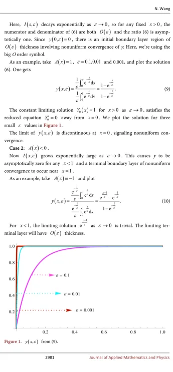
As an example, take A x

( )

≡1,

ε

=

0.1,0.01

_{and 0.001, and plot the solution}

(6). One gets

( )

0

1 1

0

1 e d _{1 e}

, .

1 e d 1 e

s

x x

s s y x

s

ε

ε ε

ε

−

− −

−

= =

−

∫

(9)

The constant limiting solution Y x0

( )

=1 for x>0 as

ε

→0, satisfies the

reduced equation Y0′ =0 away from x=0. We plot the solution for three

small ε values in Figure 1.

The limit of y x

( )

,

ε

is discontinuous at x=0, signaling nonuniform con-vergence.

Case 2: A x

( )

<0_.

Now I x

( )

,

ε

_{grows exponentially large as}

ε

→0_{. This causes}_y_{to be}

asymptotically zero for any x<1_{and a terminal boundary layer of nonuniform}

convergence to occur near x=1_.

As an example, take A x

( )

≡ −1_{and plot}

( )

1

1 1

0

1 1

1 0

e _{e d}

e e

, .

e _{e d} 1 e

s

x x

s s y x

s

ε ε

ε ε ε

ε −

− ₋

− −

−

= =

−

∫

(10)

For x<1_{, the limiting solution}exε1 −

as

ε

→0_{is trivial. The limiting}

[image:3.595.198.544.31.776.2] [image:3.595.211.533.518.733.2]

ter-minal layer will have O

( )

ε

thickness.

(4)

2. Turning Points

Case 3: A x

( )

= −x 0.5_.

Now there’s a simple turning point at x=0.5_and

( )

2 ₂

1 1 1 ₁ ₁ ₁

2 2 4 ₈ ₂ ₂

, e s e e s .

I s_ε ε ε ε

_ _      − __ − _ − _ − _ − _     = =

We write the ratio (6) as

( )

0 1 0 , d , . , d x

I s s

y x

I s s

ε ε

ε

=

∫

(11)

The exact solution is

( )

1 2 2 1

, 1 ,

2 1 2 2 x erf y x erf ε ε ε   ₋              = _ + _    _ _          (12)

where _{erf z}

( )

₌ 2 ₀ze d−t2 _t

π

∫

is the error function [14]. It satisfies

z xz

′′

+

′

=

0

,

it is odd, it increases monotonically, and it tends to ±1 as x→ ±∞_.

Since the integrands of (11) peak at the turning point and are asymptotically negligible elsewhere, we will have

( )

1 0, for

2 ,

1

1, for .

2 x y x x

ε

 _<    _> 

 (13)

The numerator and denominator of (11) are both O

( )

ε

_{. Clearly,}

1_, 1

2 2

y_

ε

 =_

  , there’s antisymmetry about

1 2

s= _{, and an}O

( )

ε

_{thick region}

of nonuniform convergence about the midpoint.

Plotting the solution (12) for _ε₌₁₀−3_{, we get}_{Figure 2}_.

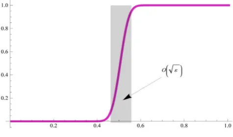
Case 4: A x

( )

= −x

α

, 0< <

α

1_.

We rescale I to get

( )

2 ₁ ₂

2 2

e−αεI s,_ε ₌e− ε s−α ,

a function that peaks in an O

( )

ε

_{interval about} s=α_{and is asymptotically}

negligible elsewhere. This implies that a shock layer of nonuniform convergence occurs about the turning point. The exact solution (6) is

( )

, 2 2 .

(5)

[image:5.595.253.491.74.214.2]

DOI: 10.4236/jamp.2019.712208 2983 Journal of Applied Mathematics and Physics Figure 2. _{y x}

(

_,10−3

)

from (12).

For

α

=1₃_and _ε₌₁₀−3_{, we get}_{Figure 3}_.

Not surprisingly, the asymptotic solution is essentially a translation of that for

0.5

α

= _{. For}

α

=0_,

( )

2 2 2 0 1 ₂ 0 e d , , e d s x s s y x s ε ε

ε

− − =

∫

(15)

so we again get an O

( )

ε

_{initial layer (see}_{Figure 4(a)}_and_{Figure 4(b)}_).

For

α

=1_{, there is an analogous terminal layer. For}

α

<0_or

α

>1_{, the}

boundary layer is O

( )

ε

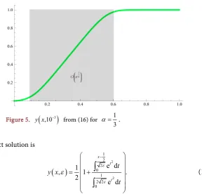
_,_i.e._thinner.

Case 5: A x

( ) (

= x−

α

)

3, 0< <

α

1_.

We have a third order turning point at x=α_{. Again, the rescaled integral}

( )

,

I s

ε

_{peaks at}s=α_{, causing}_y_{to jump there. The shock layer is now} 1

4

O_ε _

  thick. The exact solution is

( )

(

)

(

)

4 ₄

1_, 1_,

4 4 4 4

, ,

1

1_, 1_,

4 4 4 4

x y x α α ε ε ε α α ε ε  ₋  _ _  

Γ_ __{− Γ} _

 

=

 ₋  _ _

 

Γ _{− Γ} _

  _ _

 

(16)

where

( )

_, a1_{e d}u

z

a z +∞u − − u

Γ =

_∫

_{is the incomplete gamma function.}

Evaluating y x

( )

,

ε

_for 1

3

α

= _and _ε₌₁₀−3_{, we get}_{Figure 5}_.

To steepen the shock layer, we must take ε_{much smaller.}

We change the sign of A for the next three examples.

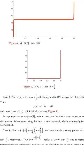
Case 6:

( )

1

2

A x = −x_.

Rewriting (6) as

(6)

(

_,10−3

)

from (14) with α=1₃_.

(a)

[image:6.595.215.528.68.717.2]

(b)

(7)

[image:7.595.238.527.67.343.2]

Figure 5. _{y x}

(

_,10−3

)

_{from (16) for} 1

3

α= .

the exact solution is

( )

2 2 1 2 2 0 1 2 2 0 e d 1

, 1 .

2 _{e d}

x t t t y x t ε ε ε −       = _ + _      

∫

(18)

We note that the solution could be expressed in terms of Dawson’s integral

( )

2 2

0 e z ze dt

F z ₌ − t

∫

. The integrands in (17) peak symmetrically at s=0_{and 1,}

being asymptotically negligible elsewhere. Moreover, y  =_{ }1₂ 1₂

  . Indeed

( )

1

2

y x  for 0< <x 1_{, and twin}O

( )

ε

boundary layers occur near both end-points. For _ε₌₁₀−3_{, we have}_{Figure 6}_.

Case 7: For

( )

, 0 1

2

A x = −α x < <α _{, we have}

( )

( ) ( ) 2 2 0 2 1 2 0 e d , . e d s s x s s s y x s α ε α ε ε − − =

∫

(19)

Its exact solution is

( )

2 2 2 2 2 2 0 0 1 2 2 0 0

e d e d

, .

e d e d

x t t t t t t y x t t α α ε ε α α ε ε ε − − + = +

∫

(20)

The integrand of (19) is asymptotically negligible for s<2

α

, but asymptoti-cally large for s>2

α

_{. This implies that}

( )

0 for 1,

y x  x<

so there is as O

( )

ε

-thick terminal layer. As an example, consider

3 1

10 0.

3

y x y

− _′′₊ ₋  _′₌

 

 

We have Figure 7 for picture of _{y x}

(

_,10−3

)

(8)

[image:8.595.206.532.74.636.2]

(

_,10−3

)

from (18).

Figure 7. _{y x}

(

_,10−3

)

_for 1

3

α= .

Case 8: For

( )

, 1

2

A x = −α x α> _{, the integrand in (19) decays for} 0< <s 2

α

_.

Thus

( )

1 for 0

y x  x>

and there is an O

( )

ε

_{thick initial layer (see}_{Figure 8}_).

For appropriate 1

( )

1

2 o

α + , we’d expect that the shock layer moves across

the interval. We’re now using the little o order symbol, which admittedly isn’t very explicit.

Case 9: For (

( )

1 3

4 4

A x =_x− _x− _

  , we have simple turning points at

1 4

and 3

4. Moreover,

( )

2

3

3 4

, e x x

I x

_ε

₌ −ε −  _{peaks at} _x₌₀_and 3

4 and is

asymp-totically negligible elsewhere. The sizes of the contributions to the integral differ, however. The area under I near x=0_is O

( )

ε

_{, but that near} 3

4

x= _is

( )

O

ε

_,_i.e._{, larger. Thus, the ratio (6) is}O

( )

ε

_for 0 3 4

x

< < _and O

( )

1

for 3 1

(9)

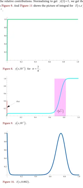
Computing for _ε₌₁₀−3_{, we get}_{Figure 9}_.

This relies on the following figures. We’ve increased ε_in_{Figure 10}_to

show the relative contributions. Normalizing to get y

( )

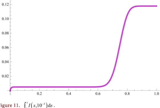
1 1= , we get the solu-tion in Figure 9. And Figure 11 shows the picture of integral for I x

( )

,

ε

_with

3 10 ε₌ − _.

Figure 8. _{y x}

(

_,10−3

)

for α=3₄_.

Figure 9. _{y x}

(

_,10−3

)

[image:9.595.233.511.106.736.2]

.

(10)

[image:10.595.233.513.72.261.2]

Figure 11.

(

3

)

0 ,10 d

x

I s − s

∫

.

3. Conclusion

We have not been exhaustive, but we have certainly demonstrated a wide variety of asymptotic solutions to turning point problems of the form (4) - (5). They mimic the asymptotics of the more general boundary layer resonance problem. When the problem of turning points becomes complicated, numerical methods will become unreliable. Finding the limiting solution is extremely ill conditioned as Trefethen recently observed. Due to the serious instability of direct numerical methods, the examples found in scattered literature are usually less detailed. In this paper, we only give asymptotic solutions for a class of singularly perturbed with a turning point. Indeed, the techniques developed here might be expected to apply to that problem. Readers are encouraged to study other limiting possi-bilities for (4) - (5).

Acknowledgements

This research is supported by the Natural Science Foundation of Shanghai Insti-tute of Technology, Research Fund nos. ZQ2018-22, 391100190016027.

Conflicts of Interest

The author declares no conflicts of interest regarding the publication of this pa-per.

References

[1] Ackerberg, R.C. and O’Malley Jr., R.E. (1970) Boundary Layer Problems Exhibiting Resonance. Studies in Applied Mathematics, 49, 277-295.

https://doi.org/10.1002/sapm1970493277

[2] Fraenkel, L.E. (1969) On the Method of Matched Asymptotic Expansions. Mathe-matical Proceedings of the Cambridge Philosophical Society, 65, 263-284.

https://doi.org/10.1017/S0305004100044236

[3] Skinner, L.A. (2011) Singular Perturbation Theory. Springer, New York.

(11)

DOI: 10.4236/jamp.2019.712208 2989 Journal of Applied Mathematics and Physics [4] Vasil’eva, A.B., Butuzov, V.F. and Kalachev, L.V. (1995) The Boundary Function

Method for Singular Perturbation Problems. SIAM, Philadelphia.

https://doi.org/10.1137/1.9781611970784

[5] Fruchard, A. and Schäfke, R. (2013) Composite Asymptotic Expansions. Lecture Notes in Mathematics. Vol. 2066, Springer, Heidelberg.

https://doi.org/10.1007/978-3-642-34035-2

[6] O’Malley, R.E. (2008) Singularly Perturbed Linear Two-Point Boundary Value Prob-lems. SIAM Review, 50, 459-482. https://doi.org/10.1137/060662058

[7] O’Malley, R.E. (2014) Historical Developments in Singular Perturbations. Springer, Cham. https://doi.org/10.1007/978-3-319-11924-3

[8] Sharma, K.K., Rai, P. and Patidar, K.C. (2013) A Review on Singularly Perturbed Differential Equations with Turning Points and Interior Layers. Applied Mathe-matics and Computation, 219, 10575-10609.

https://doi.org/10.1016/j.amc.2013.04.049

[9] Matkowsky, B.J. (2018) Singular Perturbations in Noisy Dynamical Systems. Euro-pean Journal of Applied Mathematics, 29, 570-593.

https://doi.org/10.1017/S0956792518000025

[10] Trefethen, L.N., Birkisson, A. and Driscoll, T.A. (2018) Exploring ODEs. SIAM, Philadelphia.

[11] Wasow, W. (1985) Linear Turning Point Theory. Springer, New York.

https://doi.org/10.1007/978-1-4612-1090-0

[12] Olver, F.W.J. (1974) Asymptotics and Special Functions. Academic Press, New York. [13] Wong, R. (1989) Asymptotic Approximations of Integrals. Academic Press, New York. [14] Olver, F.W.J., Lozier, D.W., Boisvert, R.F. and Clark, C.W. (2010) NIST Handbook