Spatial patterns and species coexistence
Using spatial statistics to identify underlying ecological
processes in plant communities
Calum Brown
Thesis submitted for the degree of
DOCTOR OF PHILOSOPHY
In the School of Mathematics and Statistics
UNIVERSITY OF ST ANDREWS
March 2012
1. Candidate’s declarations:
I, Calum Brown, hereby certify that this thesis, which is approximately 38,000 words in length, has been written by me, that it is the record of work carried out by me and that it has not been submitted in any previous application for a higher degree.
I was admitted as a research student in October 2008 and as a candidate for the degree of Ph.D. in October 2008; the higher study for which this is a record was carried out in the University of St Andrews between 2008 and 2012.
Date …… signature of candidate ………
2. Supervisor’s declaration:
I hereby certify that the candidate has fulfilled the conditions of the Resolution and Regulations appropriate for the degree of Ph.D. in the University of St Andrews and that the candidate is qualified to submit this thesis in application for that degree.
Date …… signature of supervisor ………
3. Permission for electronic publication: (to be signed by both candidate and supervisor)
In submitting this thesis to the University of St Andrews I understand that I am giving permission for it to be made available for use in accordance with the regulations of the University Library for the time being in force, subject to any copyright vested in the work not being affected thereby. I also understand that the title and the abstract will be published, and that a copy of the work may be made and supplied to any bona fide library or research worker, that my thesis will be electronically accessible for personal or research use unless exempt by award of an embargo as requested below, and that the library has the right to migrate my thesis into new electronic forms as required to ensure continued access to the thesis. I have obtained any third-party copyright permissions that may be required in order to allow such access and migration, or have requested the appropriate embargo below.
The following is an agreed request by candidate and supervisor regarding the electronic publication of this thesis:
(iii) Embargo on both all of printed copy and electronic copy for the same fixed period of 2 years (maximum five) on the following ground(s):
publication would preclude future publication;
ii
Abstract
The use of spatial statistics to investigate ecological processes in plant communities is becoming increasingly widespread. In diverse communities such as tropical rainforests, analysis of spatial structure may help to unravel the various processes that act and interact to maintain high levels of diversity. In particular, a number of contrasting mechanisms have been suggested to explain species coexistence, and these differ greatly in their practical implications for the ecology and conservation of tropical forests. Traditional first-order measures of community structure have proved unable to distinguish these mechanisms in practice, but statistics that describe spatial structure may be able to do so. This is of great interest and relevance as spatially explicit data become available for a range of ecological communities and analysis methods for these data become more accessible.
This thesis investigates the potential for inference about underlying ecological processes in plant communities using spatial statistics. Current methodologies for spatial analysis are reviewed and extended, and are used to characterise the spatial signals of the principal theorised mechanisms of coexistence. The sensitivity of a range of spatial statistics to these signals is assessed, and the strength of such signals in natural communities is investigated.
iv
Acknowledgements
I owe thanks to many people for help and support during my Ph.D. Firstly my supervisors, Janine Illian, David Burslem and Richard Law, who gave me the fantastic opportunity to work on this project and offered me encouragement and assistance throughout. I have learnt a great deal from them and am very grateful indeed to them all. Special thanks go to Janine for her tremendously encouraging, if at times apparently unfounded, belief in my ability to complete this thesis. This work would not have been possible without generous funding and support from Microsoft Research and, latterly, from the Centre for Research into Ecological and Environmental Modelling. This also enabled me to attend several conferences at which I benefitted from the advice of many statisticians and ecologists. My supervisor at Microsoft, Drew Purves, also provided inspiration and guidance. Thanks are due to all the Principal Investigators of rainforest plots who collaborated with me, and especially to I Fang Sun, Yu-Wen Pan and other staff and students at Tunghai University who made my visit to Taiwan so useful and memorable. I’m also grateful for technical support from a number of people, notably Tony Travis at the Aberdeen Rowett Institute of Nutrition and Health, Herbert Fruchtl in St Andrews and, especially, Phil LeFeuvre at CREEM who was always willing and able to solve any problem at a moment’s notice. Thanks to Rhona Rodger too for calmly handling a great diversity of problems which had mystified me.
I benefitted enormously from the friendly and stimulating atmosphere at CREEM and am grateful to all its members for creating such an ideal working environment - and for the plentiful supply of cake that made the period between coffee and lunch times so productive. Angelika Studeny was extremely generous with her time and mathematical expertise throughout, and provided numerous useful critiques, ideas and discussions. Glenna Evans and Cornelia Oedekoven have been consistently supportive and cheerful companions on the PhD rollercoaster, and Bruno Caneco a dependable source of much-needed amusement, advice and music.
vi
Table of Contents
Abstract………... ii
Acknowledgements………. iv
Table of contents... vi
List of figures... ix
List of tables... xii
Chapter 1 - Introduction ... 1
1.1 Species coexistence – history... 2
1.2 Niche theory ... 3
1.3 Lottery models ... 3
1.4 Janzen-Connell effect ... 4
1.5 Heteromyopia ... 4
1.6 Neutral theory ... 5
1.7 Model tests and comparisons: first-order ... 5
1.8 Model tests and comparisons: second-order ... 6
1.9 Thesis plan... 8
Chapter 2 - Linking ecological processes with spatial and non-spatial patterns in plant communities……… ... 9
2.1 Introduction ... 10
2.2 Materials and methods ... 11
2.2.1 STOCHASTIC PROCESS FOR MULTISPECIES SPATIAL PATTERNS ... 11
2.2.2 ECOLOGICAL MODELS FOR SPECIES COEXISTENCE ... 12
2.2.2.1 Neutral model ... 12
2.2.2.2 Spatial niche model ... 12
2.2.2.3 Lottery (temporal niche) model ... 13
2.2.2.4 Janzen–Connell model ... 13
2.2.2.5 Heteromyopia model ... 13
2.2.3 NUMERICAL VALUES FOR SIMULATIONS ... 14
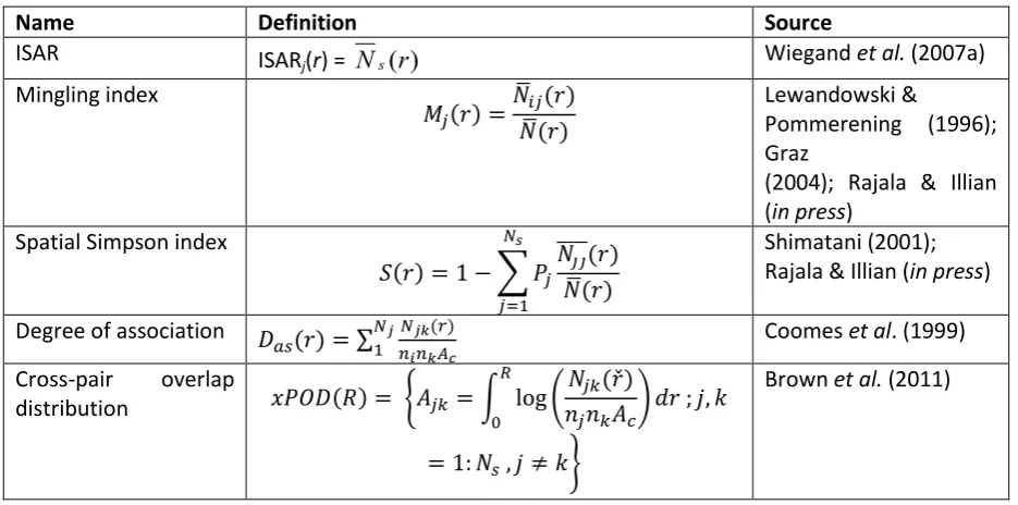
2.2.4 CROSS-PAIR OVERLAP DISTRIBUTION (xPOD) ... 15
2.2.5 COMMUNITY EVENNESS AND DIVERSITY ... 15
2.2.6 STATISTICAL INFERENCE ... 16
2.3 Results ... 18
2.3.1 ILLUSTRATIVE EXAMPLE ... 18
2.3.2 SPECIES ABUNDANCE DISTRIBUTIONS ... 18
vii
2.4 Discussion ... 26
2.5 Appendix 2.1: Definition of the pair correlation function ... 29
2.6 Appendix 2.2: Sensitivity analysis of variation in dispersal kernels ... 30
2.6.1 RESULTS & DISCUSSION ... 30
Chapter 3 - Multispecies coexistence in tropical forests: spatial signals of topographic niche differentiation increase with environmental heterogeneity ... 32
3.1 Introduction ... 33
3.2 Methods ... 34
3.2.1 DATA... 34
3.2.2 SPATIAL STATISTIC (CROSS-PAIR OVERLAP DISTRIBUTION) ... 38
3.2.3 ENVIRONMENTAL METRICS AND REGRESSION ... 40
3.3 Results ... 41
3.4 Discussion ... 44
3.5 Appendix 3.1: Calculation of cross-pair overlap distribution (xPOD) ... 47
3.6 Appendix 3.2: Additional plots ... 48
Chapter 4 - Spatial statistics for the inference of underlying process in plant communities ... 55
4.1 Introduction ... 56
4.1.1 SPATIAL STATISTICS ... 56
4.1.2 SPATIAL STRUCTURE ... 57
4.2 Methods ... 58
4.2.1 SPATIAL STATISTICS ... 58
4.2.1.1 Scattering ... 58
4.2.1.2 Exposure ... 58
4.2.2 ECOLOGICAL SIMULATIONS ... 63
4.2.3 COMPARING SPATIAL STATISTICS ... 63
4.3 Results ... 64
4.3.1 SPECIES LEVEL ... 64
4.3.1.1 Scattering ... 65
4.3.1.2 Exposure ... 72
4.3.2 COMMUNITY LEVEL... 87
4.3.2.1 Scattering ... 87
4.3.2.2 Exposure ... 92
4.4 Discussion ... 102
4.4.1 SCATTERING ... 102
4.4.2 EXPOSURE ... 103
4.4.3 LEVEL OF INFORMATION ... 106
4.4.4 GENERAL ... 106
viii
4.6 Appendix 4.1: Measures of β-diversity ... 110
4.6.1 INTRODUCTION ... 110
4.6.2 RESULTS ... 110
4.6.3 DISCUSSION ... 110
Chapter 5 - Neighbourhood effects on mortality and diversity in a tropical rainforest ... 115
5.1 Introduction ... 116
5.2 Methods ... 117
5.2.1 STUDY AREA/DATA ... 117
5.2.2 MODEL DESIGN AND SELECTION ... 118
5.3 Results ... 122
5.3.1 MODEL SELECTION CRITERIA ... 122
5.3.2 HIERARCHIES ... 122
5.3.3 SELECTED MODEL ... 125
5.4 Discussion ... 127
5.5 Appendix 5.1: Supporting plots... 132
Chapter 6 - Discussion ... 133
ix
List of figures
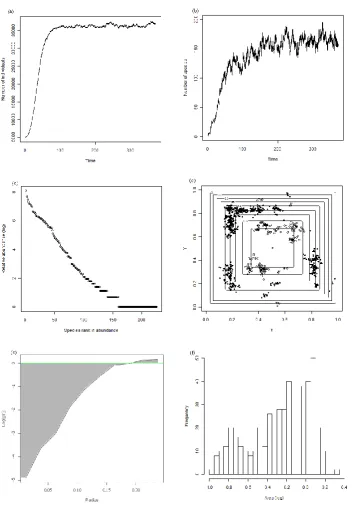
Figure 2.1. Realization of a spatial multispecies birth–death process, showing the statistics
calculated on the multispecies spatial pattern at the end. ... 17
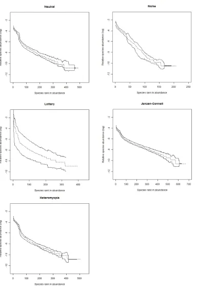
Figure 2.2. Species abundance distributions (SADs) obtained from different ecological models. ... 20
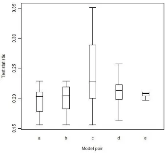
Figure 2.3. Boxplots of Kolmogorov–Smirnov test statistics. ... 21
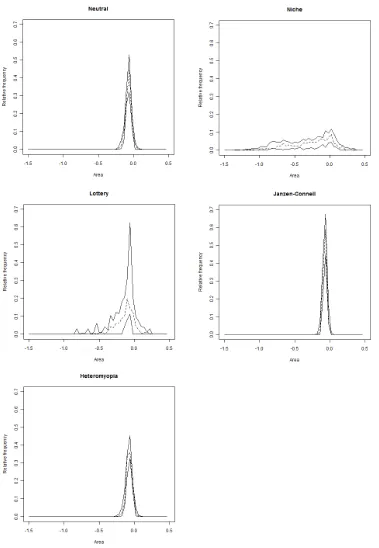
Figure 2.4. Cross pair overlap distributions (xPODs) obtained from different ecological models. ... 23
Figure 2.5. Boxplots of Kolmogorov–Smirnov test statistics obtained from comparing pairs of cross pair overlap distributions within and between ecological models. ... 25
Figure A2.2.1. Cross pair overlap distributions (xPODs) obtained from neutral and niche ecological models with a range of dispersal kernels. ... 31
Figure 3.1: The contribution of species pairs to the xPOD for Lienhuachih. ... 39
Figure 3.2: Topographies and cross-pair overlap distributions for Pasoh and Gutianshan. ... 42
Figure 3.3: Significant relationships between cross-pair overlap distribution standard deviations and environmental metrics. ... 43
Figure A3.1: Topographies and cross-pair overlap distributions for all plots. ... 49
Figure A3.2: Relationships between xPOD standard deviations and elevation range in each plot. ... 50
Figure A3.3: Relationships, fitted regression lines and their associated p-values for each of the environmental metrics against standard deviation of cross-pair overlap distributions. ... 51
Figure A3.4: Standard deviations of cross-pair overlap distributions against biogeographical variables. ... 53
Figure A3.5: The chance relationship between latitude and elevation range of plots. ... 53
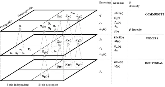
Figure 4.1: The class and level to which each piece of information used in the construction of the measures belongs. ... 62
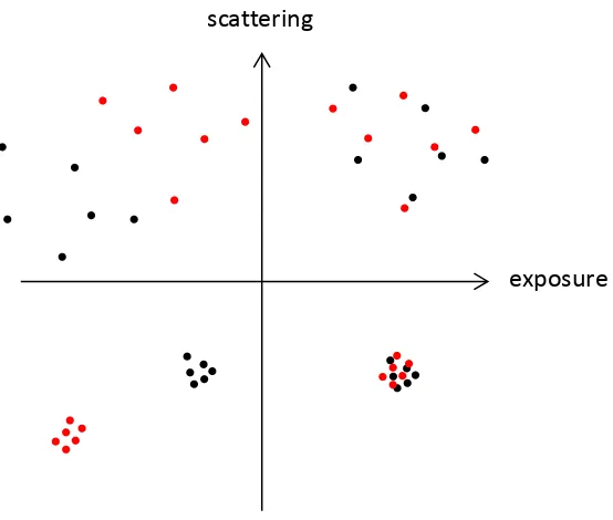
Figure 4.2: Extremes of scattering and exposure. ... 63
Figure 4.3: Measure of interspecific segregation results for each model. ... 65
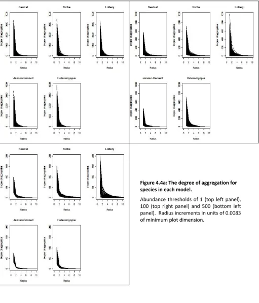
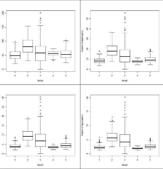
Figure 4.4a: The degree of aggregation for species in each model. ... 66
Figure 4.4b: The degree of aggregation for species in each model. ... 67
Figure 4c: Histograms of values of the degree of aggregation for species in each model. ... 68
Figure 4.5a: The proportion of conspecific neighbours for species with abundances of 500 or more in each model. ... 69
x
Figure 4.5c: Histograms of values of the proportion of conspecific neighbours for species in each
model. ... 71
Figure 4.6: Cross-pair overlap distributions for species in each model. ... 72
Figure 4.7a: ISAR curves for species with abundances of 500 or more in each model expressed in terms of species numbers and proportion of total community size. ... 74
Figure 4.7b: ISAR result boxplots for species in each model. ... 75
Figure 4.7c: Histograms of ISAR values for species in each model. ... 76
Figure 4.8a: Mingling index for species in each model. ... 78
Figure 4.8b: Mingling index boxplots for species in each model. ... 79
Figure 4.8c: Histograms of mingling index values for species in each model ... 80
Figure 4.9a: The degree of association for species in each model, at the level of species pairs... 81
Figure 4.9b: Degree of association boxplots for species pairs in each model. ... 82
Figure 4.9c: Histograms of degree of association values for species pairs in each model ... 83
Figure 4.10a: The degree of association for species in each model, at species level. ... 84
Figure 4.10b: Degree of association boxplots for species in each model. ... 85
Figure 4.10c: Histograms of degree of association values for species in each model ... 86
Figure 4.11a: Prediction intervals (95%) for the degree of aggregation (summed) at community level. ... 88
Figure 4.11b: Boxplots of degree of aggregation (summed) values ... 88
Figure 4.12a: Prediction intervals (95%) for the mean degree of aggregation at community level .... 89
Figure 4.12b: Boxplots of degree of aggregation mean values. ... 89
Figure 4.13: Boxplots of mean values of the measure of interspecific segregation for each model. .. 90
Figure 4.14a: Prediction intervals (95%) for the mean proportion of conspecific neighbours at community level... 91
Figure 4.14b: Boxplots of mean values of the proportion of conspecific neighbours for each model. 91 Figure 4.15a: Prediction intervals (95%) for the spatial Simpson index ... 92
Figure 4.15b: Boxplots of spatial Simpson indices for each model ... 93
Figure 4.16a: Prediction intervals (95%) for the spatial Simpson index ... 93
xi
Figure 4.17a: Prediction intervals (95%) for the cross-pair overlap distribution. ... 95
Figure 4.17b: Boxplots of means and standard deviations of the cross-pair overlap distribution ... 96
Figure 4.18a: Prediction intervals (95%) for the mean ISAR at community level, as a proportion of total community size ... 97
Figure 4.18b: Boxplots of mean values of the ISAR, as a proportion of community size ... 98
Figure 4.19a: Prediction intervals (95%) for the mean mingling index at community level... 99
Figure 4.19b: Boxplots of mean values of the mingling index for each model. ... 100
Figure 4.20a: Prediction intervals (95%) for the mean degree of association at community level .... 101
Figure 4.20b: Boxplots of mean values of the degree of association for each model... 101
Figure 4.21: A 3-D plot of results from each model based on mean (community-level) values of the mingling index, proportion of conspecific neighbours, and standard deviation of the xPOD. ... 108
Figure A4.1: The labelling of cells or quadrats used for the calculation of measures of beta-diversity. ... 112
Figure A4.2: Example results for measures of beta-diversity, typical of the three types of curve produced by the 21 measures considered. ... 113
Figure A4.3: Boxplots of estimated values of parameter alpha in the power law which best fits results for 3 measures of beta diversity in each model. ... 114
Figure 5.1: Model selection criteria against model complexity. ... 123
Figure 5.2: Training and test data likelihoods for the five models with the highest test data maximum likelihoods, with and without hierarchies. ... 124
Figure 5.3: Posterior 95% credible intervals for the species-specific intrinsic mortality parameter with and without a hierarchy. ... 124
Figure 5.4: Significant (non-zero) posterior 95% credible intervals for the neighbour diameter parameter. ... 126
Figure 5.5 Significant (non-zero) posterior 95% credible intervals for the neighbour phylogenetic relatedness parameter ... 126
Figure 5.6: Diameter (dbh) ranges for species with significant phylogenetic and neighbour-diameter effects. ... 129
Figure 5.7: The range of Clark & Evans aggregation index values produced by species with significant phylogenetic and neighbour-diameter effects. ... 130
Figure A5.1: Test data likelihood values for the three most successful models:... 132
xii
List of tables
Table 2.1. Parameters for ecological models. ... 14
Table 2.2. Mean evenness and diversity of each model. ... 19
Table 2.3. Mean and 90% limit values of the Kolmogorov–Smirnov test statistic comparing pairs of SADs within and between contrasting models of ecological interactions, using species of all abundances. ... 22
Table 2.4. Mean and 90% limit values of the Kolmogorov–Smirnov test statistic comparing pairs of SADs within and between contrasting models of ecological interactions, using an abundance threshold of 500 individuals. ... 22
Table 2.5. Mean, standard deviations and skewness of cross pair overlap distributions for contrasting models of ecological interactions. ... 24
Table 2.6. Mean and 90% limit values of the Kolmogorov–Smirnov test statistic comparing pairs of xPODs within and between contrasting models of ecological interactions. ... 24
Table A2.2.1. Parameters for ecological models. ... 30
Table 3.1: Summaries of the plots included in the analyses ... 36
Table 3.2: The names, identities and characteristics described by the environmental metrics calculated for each plot. ... 41
Table A3.1: p-values for single linear regressions of environmental metrics against moments of species abundance distributions (SAD) and the Shannon diversity index for each plot... 54
Table 4.1: Separate pieces of information used in spatial measures ... 60
Table 4.2a: Definitions of measures of scattering ... 60
Table 4.2b: Definitions of measures of exposure ... 61
Table 4.3: Means, standard deviations and skews of the degree of aggregation for species in each model with an abundance threshold of 500. ... 68
Table 4.4: Means, standard deviations and skews of the proportion of conspecific neighbours for species in each model with an abundance threshold of 500. ... 71
Table 4.5: Means, standard deviations and skews of xPODs for species in each model, with an abundance threshold of 500. ... 73
Table 4.6: Means, standard deviations and skews of ISAR values for species in each model with an abundance threshold of 500. ... 76
Table 4.7: Means, standard deviations and skews of mingling index results for species in each model, with an abundance threshold of 500. ... 80
xiii
1
2
One of the major goals of modern conservation is the preservation of biological diversity, the variation in life at genetic, organism and species levels, at the global scale (Magurran 2004; IUCN 2011). Despite being a priority in national and international policy around the world (e.g. Scottish Executive 2004; JNCC 2011; UNEP 2012), this objective is perhaps most closely associated with the conservation of tropical rainforests. Estimated to contain more than half of Earth’s species of land plants and animals, these forests are under intense pressure from logging, hunting and the conversion of land for pastoral and arable agriculture (Wilson 1985; Skole & Tucker 1993; Whitmore 1998; Primack & Corlett 2005). Attempts to stem the ongoing loss of rainforests to anthropogenic activities like these are many and varied, but share a focus on the protection of relatively pristine areas intended to act as reservoirs of diversity (Turner 1996; Myers et al. 2011). Beyond this broad and large-scale approach, conservation efforts are supported by relatively little ecological theory or empirical evidence. In particular, attempts to maintain the extraordinary levels of species diversity found in the tropics are hampered by a fundamental lack of understanding of the processes responsible for generating and supporting this diversity (Connell 1978; Chesson 2000; Burslem et al.
2005). Despite having been an important focus of study throughout the history of ecology, species coexistence in tropical rainforests remains largely unexplained.
1.1 Species coexistence – history
Mechanisms that support the coexistence of species have been the subject of study throughout the history of ecology, and many modern explanations were anticipated by early work on this subject. Darwin famously warned against the interpretation of an ‘entangled bank’ of vegetation as a randomly assembled group of species, suggesting instead that it was the product of deterministic processes through which each species had evolved a unique role within the community (Darwin, 1859). Until a fuller understanding of genetics came to underpin evolutionary theory, however, explanations focused on the physiological ability of plants to live in particular environmental conditions. Eugenius Warming, another of ecology’s founding figures, influentially argued that both current and previous conditions dictated species’ observed distributions (Warming 1895). The greater the ability of plants to adapt to prevailing conditions, the more important these became for shaping species distributions (Warming 1895; Collins et al. 1986).
The rediscovery of Gregor Mendel’s genetic experiments (Mendel 1865) dispelled much of the scepticism about evolution by natural selection and suggested that adaptation through genetic variation was a general, rapid and powerful process (Osborn 1926). Darwin’s earlier portrayal of a community as a tightly packed matrix of ‘wedges’, representing species with different environmental requirements that shape and displace one another, also received support. If genetic variation allowed organisms to evolve according to environmental pressures, they could equally respond to the pressures of other, competing, members of their community (Darwin 1859, Kingsland 1985). Coexistence was therefore a matter of both the environmental and interactive ‘fit’ of species (von Humboldt & Bonpland, 1805).
3
1.2 Niche theory
The work of Darwin, Warming and others led to the development of niche-assembly theories, in which coexistence was explained by species’ differing specialisations (initially in terms of habitat). Prominent among the early developers of this theory was Grinnell (e.g. 1917), who expressed a general consensus that “each animal occupies a definite area, that is, has a habitat or range, which is distinctive enough to be included among the characters of the species and described along with its habits and the features of its bodily structure” (p115). This environmental, spatial view of niches was extended by others (e.g. Elton, 1927) to include the functional role of each species, and so was defined with reference to the interactions within a community. As a result, competition increasingly became viewed as central to the niche concept. Gause’s (1934) competitive exclusion principle, building on the theories of Darwin (1859), Grinnell (1904) and, especially, Volterra (1926) and Lotka (1932), formalised this and suggested that coexistence of species required each to have its own unique environmental and interactive niche.
This niche concept was typified by Hutchinson (1958) who expressed the purely environmental, abiotic domain of a species as its ‘fundamental niche’ and its actual range, constrained by interactive, biotic factors as its ‘realised niche’. Each represented a hypervolume with dimensions determined by environmental variables and interactions, and each hypervolume was distinct, even if only because of competition within identical fundamental niches. This was supported by subsequent research into the stabilising effect of predation on competitive interactions that would otherwise result in the exclusion of species (Slobodkin 1961, 1964). Diamond’s (1975) community assembly rules held that a community was formed when species are “coadjusted in their niches and abundances, so as to fit with each other and resist invaders” (p343).
Empirical tests of this form of niche theory faced two difficulties. Firstly, Hutchinson’s formulation predicted that even where species appeared to share identical niches, they would in fact differ in some unobserved – and potentially unobservable – way. Secondly, the fundamental niche was by its nature unobservable except in the absence of biotic interactions, and therefore effectively impossible to investigate, confirm or disprove (Andrewartha 1958). These problems were particularly substantial because competition between species was not often apparent. Hutchinson himself noted the “extreme difficulty of identifying competition as a process actually occurring in nature” (Hutchinson, 1958, p418), and that competitive exclusion may be circumvented by migration and random or cyclical disturbances (also noted by e.g. Gleason 1939). As a result, the established view of community structure as an expression of deterministic niche assembly processes began to be questioned (e.g. Gleason 1939; Williams 1964).
1.3 Lottery models
4
This argument formed the basis of lottery models, which assume that temporal environmental variance benefits different species at different times through niche availability. The first of these models was developed by Sale (1977) and quickly extended by others (e.g. Chesson & Warner, 1981; Chesson & Huntly, 1988). They attracted attention in part because the lottery model was the only coexistence theory to include environmental stochasticity over time (Hatfield et al. 1996). It also did not depend upon small and cryptic differences between niches as the established niche-differentiation theory did, suggesting only that species differed in their response to environmental change. Even this, of course, depended upon the existence of numerous distinct niches, and so lottery models did still represent coexistence purely as a function of species-specific environmental specialisation.
1.4 Janzen-Connell effect
The difficulties associated with the interactive components of niche theory did not lead only to a focus on environmental effects. Deterministic models of species interactions continued to develop, and suggested that competition could indeed play a central role in structuring communities (Connell 1975; Sugihara 1980; Engen & Lande 1996a). Particularly influential was the work of Janzen (1970) and Connell (1970), who independently sought to explain observed low densities and unexpectedly uniform dispersions of tropical tree species. They invoked species-specific herbivory to produce overcompensating density-dependent mortality, in which young plants are unable to survive in the immediate vicinity of their parents. In addition to explaining observed spatial structure, this effect would prevent dominance by a small number of common species, promote spatial mixing of species and, crucially, support species coexistence (Connell et al. 1984).
Considerable empirical support was found for the Janzen-Connell effect. High local densities were shown to affect growth and mortality in tropical trees (Bella 1971; Diggle 1976), and additional agents of conspecific density-dependent mortality were identified in pests and pathogens (e.g. Augspurger 1983). It was expected that common species would suffer disproportionately because of the large populations of pests, predators and pathogens that they could support (Ridley 1930), and experimental studies that manipulated densities of isolated species lent support to this (e.g. Connell 1970; Augspurger 1983; Schupp 1992; Bagchi et al. 2010). On larger scales, however, evidence for Janzen-Connell effects is not compelling, with the majority of species showing no evidence of them (e.g. Hyatt et al. 2003). This has called into question the theory’s ability to explain coexistence in highly diverse communities (Lambers et al. 2002).
1.5 Heteromyopia
A recently-proposed variant of the Janzen-Connell effect, heteromyopia describes the tendency of conspecifics to interact over greater distances than heterospecifics (Murrell & Law 2003). This is relevant to coexistence because it suggests that large-scale rather than local density may affect species’ mortality rates. Depending upon the dispersal abilities of species-specific pests, predators and pathogens, this may be able to more accurately describe the previously noted disproportionate mortality expected in common species and the community compensatory trends that result (Ridley 1930; Connell et al. 1984; Amarasekare 2003; Queenborough et al. 2007).
5
compensatory trends consistent with heteromyopia being identified in some cases (Okuda et al.
1997; Webb & Peart 1999; Queenborough et al. 2007) but not in many others (He et al. 1997; Comita et al. 2010; Metz et al. 2010). The concept’s success in describing real community dynamics and explaining species coexistence is therefore uncertain.
1.6 Neutral theory
The difficulties in providing adequate explanations of coexistence using the established theories outlined above prompted the development of neutral theories intended to act as null models of coexistence (Caswell 1976; Hubbell 1979, 2001; Bell 2001). They too have deep roots in ecology. Darwin, despite arguing that deterministic processes were responsible for coexistence, acknowledged that the number and complexity of these could make community dynamics appear random (Darwin 1859). Hutchinson, even while developing what would become an archetypal expression of niche theory, similarly felt that “individual and unpredictable complexities in the determination of the niche boundaries…[mean] that in any overall view, the process would appear random” (1959, p154).
This was clearly not a contentious observation in itself, but neither did it provide a robust basis for testing the extent to which real communities were structured by non-random processes. This would instead come from the neutral model of population genetics, in which the spread of neutral mutations through a population was used as a null model for evolution by natural selection (e.g. Feller, 1951; Moran, 1958). The papers of Karlin & McGregor (1967) and Kimura (1968) are generally regarded as the first true neutral models of population genetics. These and others (e.g. Kimura, 1986; Hudson et al., 1987) can largely be adapted to ecology simply by changing the names of their variables so that genes, for example, become species (Chave 2004).
The first fully neutral model in ecology was published by Caswell (1976; based on Ewens 1972). It was able to produce relative abundance distributions that matched the log-series distribution that was among those considered empirically accurate (Fisher et al., 1943; Taylor et al. 1976). It was also able to predict very high levels of diversity, challenging the perceived importance of competition. The model was adapted by Hubbell (1979), who relaxed Caswell’s assumption of an infinite species pool and defined neutrality as ecological equivalence at the individual level, precluding any species-specific behaviour. He found that a wide range of relative abundance patterns could be produced and matched to observations by this theory.
Following this, a number of models were developed which included some neutral behaviour (e.g. Goldberg & Werner 1983; Graves & Gotelli 1983; Leigh et al. 1993; Terborgh et al. 1996), but most found that at least some non-neutral processes were necessary to explain empirical data. Hubbell’s updated neutral theory (1997; 2001) answered these criticisms by introducing a metacommunity in which speciation could occur and from which species could immigrate to the modelled community. This model was able to match a wide range of empirical species abundance distributions and has since become a focus of research, with 3212 papers citing Hubbell’s 2001 book (Google Scholar, 6/03/12).
1.7 Model tests and comparisons: first-order (non-spatial)
6
established as a test of niche-assembly theories (Bulmer, 1974; Engen & Lande, 1996a, b; May, 1976). The fact that SADs take a similar ‘hollow-curve’ shape in almost all known ecological communities has often been interpreted as evidence of their suitability for model testing (McGill et al. 2007).
First-order descriptions of community structure of this kind (relating to non-spatial properties of groups of individuals) have generally been the focus of model validation and comparison in ecology. This is partly due to the fact that they represent manageable descriptions of complex systems (Williams 1964; May 1981), but also because they are interpretable as expressions of general underlying mathematical laws. The search for laws of this kind motivated a great deal of early research in ecology (e.g. Volterra 1926; Lotka 1932), and prompted research into purely mathematical descriptions of species abundance patterns (e.g. Fisher et al. 1943). Debates about the appropriate mathematical function for fitting SADs and species-area curves are ongoing (Preston 1948; Bramson et al. 1996; 1998; McGill 2003).
Attempts to link these mathematical descriptions to particular ecological processes soon began, however (e.g. Kendall 1948). In fact, the first descriptions of SADs were mechanistic, usually being based on niche theory (Raunkiaer 1909; Smith 1913; Motomura 1932; MacArthur 1957). These became increasingly complex, but their ability to match empirical patterns did not improve substantially (Bulmer, 1974; Sugihara, 1980; Tokeshi, 1990; Marquet et al., 2003), and Hubbell’s (2001) neutral theory, which generates a zero-sum multinomial distribution of abundances, was found to be at least as successful as any of these.
Nevertheless, research of this kind has often been criticised for the apparent lack of insight that it provides. Hurlbert (1971) was among the first to express scepticism about the interpretability of numerical values or indices generated by theoretical distributions. Lepš (1990) argued that species abundance distributions are “able neither to detect nor to measure the biological interaction within a community” (p7). Neutral models in particular have been criticised as exercises in “fitting a relatively flexible mathematical function to a limited set of rank-abundance relationships” (Ricklefs 2006, p186). Nevertheless, the ability of a parsimonious theory such as neutrality to match some community characteristics at least as well as more complex and supposedly realistic models does recommend it, at least, as a suitable null model of community structure (Hubbell 2001). It may therefore be used to develop testable predictions which distinguish neutrality from other proposed mechanisms of coexistence. What is undoubtedly true is that the SAD and other first-order descriptions of community structure do not provide useful tests for such predictions, being unable to falsify any of a large number of contrasting theories about community dynamics (Vallade & Houchmandzadeh 2003; Volkov et al. 2003; McGill et al. 2007).
1.8 Model tests and comparisons: second-order (spatial)
While first-order descriptions of plant community structure have been the focus of model development and testing, research into spatial structure is equally well-established. Its importance has long been recognised (e.g. von Humboldt & Bonpland, 1805; de Candolle 1821), and rigorous descriptions of second-order structure (relating to the spatial properties of pairs of individuals) were developed alongside those of first-order structure discussed above (Watt 1947; Clark & Evans 1954; Hurlbert 1971). In recent years, however, the majority of these have come from statistical spatial point process theory, which, although partly motivated by ecology, has developed largely independently of it (Stoyan & Penttinen 2000).
7
Whittaker (1960; 1972) and subsequently by many others (e.g. Legendre & Legendre 1998; Nekola & White 1999; Koleff et al. 2003; Legendre et al. 2005), such measures continue to be used in studies of coexistence mechanisms and other general processes (Terborgh et al. 1996; Chave & Leigh 2002; Condit et al. 2002; Dornelas et al. 2006). They effectively span the classes of first- and second-order measures, containing information on spatial structure that is aggregated to some sub-global level. This makes them particularly suitable where spatial signals are of interest but practical or computational limits prevent the use of fully spatially-explicit data. Such limits are increasingly absent, however, resulting in a shift away from measures of β-diversity in studies of community structure (e.g. Condit et al. 2000).
Spatial point process methodology, in contrast, allows for the analysis and description of patterns formed by the precise locations of individuals in space. Mathematically, these patterns may be described as realisations of a random variable referred to as a spatial point process (Illian et al. 2008). Because the formulation of a process controls the characteristics of the resulting patterns, it can be used both descriptively and for modelling. The descriptive use of spatial point process methods has been dominant in ecology, and is the focus of this thesis. Nevertheless, a wide range of spatial point process models are available (Cox 1955; Stoyan & Stoyan 1994; Møller et al. 1998; Van Lieshout 2000; Illian et al. 2008) and it is increasingly possible to fit these to ecological data with highly informative results (e.g. Baddeley & Turner 2005; Guan 2006; Rue et al. 2009; Illian et al. in press).
In some cases, the application of statistics originating in spatial point process theory to forest ecology has occurred alongside their development (Matérn 1960; Ripley 1976; 1977). They have generally been used to formally describe patterns of interest such as the associations between different species (Ogata & Tanemura 1985; Wiegand et al. 2007a), clustering in mortality (Sterner et al. 1986; Queenborough et al. 2007), patterns of colonisation (Salonen et al. 1992) and to try and separate the effects of local dispersal, species interactions and environmental niche differentiation (Tuomisto et al. 2003; Hardy & Sonké 2004; Wiegand et al. 2007b).
Although these applications have shown that spatial statistics can suggest underlying ecological processes, their use in formal inferential tests of these has remained rare. Indeed, this has often been discouraged because of the possibility that different processes can generate similar or identical spatial patterns (Baddeley & Silverman 1984; Shipley & Keddy 1987; Stoyan & Penttinen 2000; Coomes et al. 1999). Lepš (1990), for example, argued that “mechanisms can be suggested on the basis of observed patterns, but they cannot be tested” (p9).
8
underlying process than the first-order patterns traditionally used (Illian et al. 2008; Law et al. 2009). Given this, a systematic investigation of the informative potential of spatial structure is required.
1.9 Thesis plan
This thesis seeks to examine the scope for detecting and distinguishing underlying ecological processes of the kind thought to explain species coexistence in tropical rainforests using spatial statistics. We will investigate the links between particular processes and the spatial structure of forest communities using established and newly developed summaries of spatial structure. We do so in order to develop robust methods of inferring underlying processes from resulting spatial patterns, with the ultimate aim of contributing to a resolution of the debate about the mechanisms of species coexistence. The principal theorised coexistence mechanisms described above have all proved able to match several observed first-order characteristics of ecological communities, and this has hampered efforts to determine which of them are accurate. The degree to which they can be distinguished by their spatial signals has not previously been systematically assessed, however. In Chapter 2 we attempt to do this using a stochastic individual-based model to generate spatially explicit data under each ecological process in isolation.
In Chapter 3, we go on to look for spatial signals in empirical data from a range of tropical rainforest plots, using the spatial statistic developed in Chapter 2. Different spatial predictions are generated by neutral and niche theories, with the structure of niche-assembled communities expected to vary systematically with the environment and the structure of neutral communities expected not to. We therefore test a prediction derived from niche theory that increasing topographical heterogeneity in tropical rainforests should lead to an increasing spatial spread of species along elevational gradients. No single summary statistic is expected to be sensitive to all forms of spatial structure, and so we compare the performance of several established spatial statistics in Chapter 4. We do this on the basis of the simulated data in Chapter 2, where each process is again known to be operating in isolation. Our aim here is twofold: to find which pieces of information and statistical summaries of spatial structure are best able to distinguish mechanisms of coexistence, and what the full spatial implications of each of these mechanisms are. We do not consider an exhaustive range of spatial statistics but only those that are representative of widely used types, relying on particular spatial measurements. Those that perform best in this comparison are expected to form the basis for a probability-based test for underlying process.
In Chapter 5 we focus on the operation of one particular process, the Janzen-Connell effect, in a real rainforest community. Having a range of potential forms and extents, the scope for identifying this effect by its spatial signals is uncertain, and so the aim of this chapter is to investigate the strength and scale of these signals. We use hierarchical Bayesian models of empirical mortality data with respect to small-scale spatial structure so that the likelihood of identifying spatial signals can be estimated.
9
CHAPTER 2 -
Linking ecological processes with spatial and non-spatial
patterns in plant communities
The work presented in this chapter has been published in:
Brown, C., Law, R., Illian, J.B. & Burslem, D.F.R.P. 2011, "Linking ecological processes with spatial and non-spatial patterns in plant communities", Journal of Ecology, vol. 99, no. 6, pp. 1402-1414.
10
2.1 Introduction
A great deal of research in ecology tries to infer ecological processes from patterns observed in nature, and this is one objective of this thesis. In community ecology, the species abundance distribution (SAD) has received particular attention, as discussed in Chapter 1 (also see e.g. McGill et al. 2007). A SAD describes the absolute or relative abundances of species in a community and is found to conform to a near-universal ‘hollow curve’ shape, comprising a small number of common species and a large number of rare ones. There is no obvious a priori reason to expect this shape, and the detailed features of SADs have therefore been used to discriminate between underlying processes, such as those involved in species coexistence. This work began with theories of niche assembly (e.g. Motomura 1932; MacArthur 1957; Tokeshi 1990), and more recently comparing SADs has become a key tool for validating the neutral theory against observed data from ecological communities (Hubbell 1979; 1997; 2001; Chapter 1).
As discussed above, a single ecological process can produce rather variable SADs (Magurran 2005;
Williamson & Gaston 2005;Volkov et al. 2005; Chapter 1), making the detection of processes from empirically derived SADs difficult (McGill et al. 2007). This is not surprising: a SAD is, after all, just a description of species’ relative abundances averaged over space. Processes affecting coexistence rely on spatial proximity of individuals, especially in sessile organisms, and SADs convey no information on spatial structure. In the context of a spatial analysis of communities, a SAD would be said to be a first-order measure (Illian et al. 2008).
A motivating assumption of this thesis is that spatial correlations ought to provide a more sensitive indicator of ecological interactions among plant species because of the importance of interactions as drivers of spatial pattern in plant communities (Bolker & Pacala 1997; Murrell & Law 2003; Wiegand
et al. 2007a). There is a long history in plant ecology of using spatial pattern to gain insight into ecological processes (e.g. Watt 1947; Clark & Evans 1954; Sterner et al. 1986), and indeed this was one motivation for the development of spatial point process methods (Matérn 1960; Ripley 1977; Stoyan & Penttinen 2000). It would be unrealistic to expect a unique mapping from a spatio-temporal process to a spatial pattern because of the array of biotic and abiotic factors at play (e.g. Baddeley & Silverman 1984; Lepš 1990), but it is reasonable to ask whether an analysis that makes use of spatial structure is a better discriminator among ecological mechanisms than one based on SADs that ignores this information.
Ecologists do often have far more information at their disposal than just that needed to construct SADs. For example, several complete spatial censuses exist for tropical rainforest trees on the 50-ha plot at Barro Colorado Island (BCI) in Panama (Hubbell et al. 2005) and numerous other sites (Losos & Leigh 2004). In the search for evidence about underlying processes on these plots, it should be possible to go beyond SADs (e.g. Hubbell 2001; Volkov et al. 2003; Etienne & Olff 2005; He 2005) to second-order measures such as spatial correlations that make use of this spatial information. The potential of these has been recognized in studies of the roles of seed dispersal and habitat heterogeneity (Condit et al. 2000; John et al. 2007), the aggregations produced by neighbourhood recruitment and mortality (Hubbell et al. 2001; Uriarte et al. 2005), and spatial patterns in diversity (Weigand et al. 2007b). It is also further investigated in Chapters 3 and 4 of this thesis. Elsewhere, temporal patterns have been used to discriminate between neutral and non-neutral mechanisms for maintaining the structure and diversity of communities (e.g. Clark & McLachlan 2003; McGill et al. 2005), as have comparisons between different spatial scales (Gilbert & Lechowicz 2004; Dornelas et al. 2006; McGill et al. 2006). However, a systematic analysis of the spatial signatures generated by different kinds of species interaction has not previously been attempted.
11
interactions (as described in Chapter 1). Our baseline was the neutral model, with its assumption of
per capita ecological equivalence between species (Hubbell 2001). Two niche models were included: a conventional niche model in which species favour specific environmental conditions that are defined spatially (e.g. Grinnell 1917; Hutchinson 1958; Zillio & Condit 2007), and a lottery model in which temporal environmental variance favours different species at different times (Sale 1977; Chesson & Warner 1981; Chesson & Huntly 1988). The Janzen–Connell hypothesis, according to which young plants suffer increased mortality in the neighbourhood of their parents, was also implemented (Janzen 1970; Connell 1970), as was a purely spatial heteromyopia model in which interspecific competition occurs over shorter distances than intra-specific competition (Murrell & Law 2003).
We generated multispecies spatial patterns through realisations of spatio-temporal stochastic processes (stochastic individual-based models) using the different underlying models of ecological interactions. At first order, we computed SADs on these spatial patterns. At second order, we computed a new community-level measure of species segregation, built from spatial pair-correlation functions, referred to as the cross-pair overlap distribution (xPOD). The xPOD will be used repeatedly throughout this thesis.
First-order signals of the modelled ecological interactions were expected to be limited given the inherent variability of SADs. Some differences in community diversity and evenness were anticipated, but were difficult to predict because the relative strength of each form of interaction in promoting coexistence has not previously been assessed. Second-order spatial signals were expected to be substantially stronger, and to take a more predictable form for each model. In particular, the spatial niche model was expected to increase the segregation among species, while the Janzen–Connell model was predicted to constrain conspecific clumping and so have the opposite effect (Chapter 5 further investigates the spatial signals of the Janzen-Connell effect).
2.2 Materials and methods
2.2.1 STOCHASTIC PROCESS FOR MULTISPECIES SPATIAL PATTERNS
Multispecies spatial patterns were obtained from realisations of a stochastic individual-based model (IBM) of a plant community based on a method in Law & Dieckmann (2000). This model will be used again in Chapter 4 and the description provided here is also relevant there. In this setting, individuals occur at discrete points x = (x1,x2); x1,x2 [0,1] in a continuous two-dimensional space. The space comprises an arena of unit area with periodic boundaries, so forming a torus and preventing the inward propagation of edge effects. The spatial pattern pi(x,t) of a species i at time t,
t R+, comprises the locations of all individuals of species i, and the multispecies pattern p(x,t) is the union of all these single-species patterns. Birth and death events take place in continuous time, together with occasional arrival of new species, so the multispecies spatial pattern changes at every event. The effect of particular assumptions about ecological interactions on the multispecies spatial pattern is investigated after a large number of birth and death events have taken place.
For simplicity, the birth process is common to all species, independent of location in the arena, and comprises an intrinsic probability per unit time b of producing an offspring, and a function m(x – x') giving the probability of the offspring being located at x' for a parent at x. Thus the probability per unit time B(x,x') of a parent at x producing an offspring at x' is
12
In a community of finite size, there would be a gradual erosion of species diversity as extinctions take place. To counter this, a low constant probability per unit time of immigration of a new species is assumed, and the location of the new individual is chosen uniformly at random in the arena. The death process is designed to allow various models of interactions among plants and is therefore more intricate. The probability per unit time of death Di(x,p) of an individual of species i at point x is:
Di(x,p) =
j
ij j
ij ij
i d w p t d
d ' (x' x)[ (x,' )
x(x')] x' eqn 2.2Here di is an intrinsic probability per unit time of death of an individual of species i. The term inside the integral takes a neighbour of species j located at x', and attaches weight wij(x'-x), which depends on the displacement x' - x of the neighbour from the target individual of species i located at x, allowing the distance over which individuals interact to depend on the species identity of the target and neighbour. The integral adds up the effect of all neighbours of species j on the target, and is given a weight d’ij, so that interaction strength can also depend on the species identities. The summation adds the effects over all neighbour species j. In the case where j = i, the neighbours are conspecifics and the product δijδx(x'), a Kronecker delta and Dirac delta function, is needed so that
the target individual is not counted as a neighbour of itself.
Spatial structure in the community comes ultimately from local dispersal and local competition, assumed to be bivariate Gaussian functions
m(x - x') =
2 22
2
σ
'
exp
σ
2
1
b bx
x
, eqn 2.3wij(x'-x) =
2 22
2
σ
'
exp
σ
2
1
ij ij d dx
x
, eqn 2.4normalized to make the volume = 1. The parameters σband σdij give the width of the distributions;
small values indicate, respectively, that offspring are dispersed close to their parent and that competition occurs with close neighbours.
2.2.2 ECOLOGICAL MODELS FOR SPECIES COEXISTENCE
2.2.2.1 Neutral model
This is the simplest model and provides a standard against which to test the others. It was implemented by making the parameters b, d, σb and σdij constant and identical for every individual irrespective of species (Section 1.6; Table 2.1).
2.2.2.2 Spatial niche model
13
2 2 2 15
.
0
1
2
5
.
0
1
2
x
x
h
x otherwise 5 . 0 5 . 0 21 x
x
eqn 2.5
This produces an environment in which the spatial extent of each specific value, and hence the size of each potential niche, is approximately equal, ensuring that any spatial signal produced is attributable to the niche process rather than environmental availability (see Fig. 2.1d).
The spatial niche model requires species to respond to the environment in different ways, so the niches of species are set by environment-dependent intrinsic death rates. Each species i is assigned a uniformly distributed random number in the range [0,1] to give it a preferred niche hi0. An individual in this optimal environment has a death probability di as in the neutral model. The dependence of the death rate on the environment is made explicit here by writing it as di (x) for an individual of species i located at a point x where the environment has a 'height' hx. The value of di (x)
is assumed to have an inverted Gaussian shape around the birth rate b, determined by the deviation
hx - hi0 from the species' preferred niche, so that di (x) is minimized at hi0:
di (x) =
20 22
2
σ
)
(
exp
σ
2
)
(
n i ni
h
h
d
b
b
x
eqn 2.6This means that, as the environment departs further from the preferred niche, the death rate of species i increases, eventually becoming the same as its birth rate and preventing it from becoming established. The parameter σn is a niche-width parameter common to all species. Thus, as σn
becomes large, species do not perceive the landscape and the dynamics are as in the neutral model. Decreasing σn makes the success of each species increasingly dependent upon it being within its
preferred niche hi0.
2.2.2.3 Lottery (temporal niche) model
This model differs from the neutral model in that the intrinsic death rates di of species are drawn from a uniform distribution centred on that of the neutral model. The environment has a low, constant probability per unit time of changing, set at 510-5. When the environment changes, new values of di for each species are drawn from the uniform distribution. As the range of the uniform distribution tends to zero, the behaviour tends to the neutral model; increasing the range makes the lottery effect stronger.
2.2.2.4 Janzen–Connell model
This model requires local dispersal of propagules, applied here when the parameter of the dispersal function is sufficiently small. It also requires a higher death rate in the presence of conspecific neighbours than in the presence of heterospecific ones, due to host-specific enemies (Janzen 1970; Connell 1970; Section 1.4). We do not model host-specific enemies, and so the Janzen–Connell mechanism is introduced by making the neighbourhood conspecific death term d'ii larger than the
heterospecific one d'ij. In the natural environment, a distinction also would be made between the
parent and the offspring, but we do not do this because age and size of individuals are not specified under the simple conditions of the stochastic process.
2.2.2.5 Heteromyopia model
14
2.2.3 NUMERICAL VALUES FOR SIMULATIONS
Each realization starts with 50 species of 100 individuals (5000 individuals in total), distributed independently and uniformly at random in the arena. The spatial pattern is updated by birth and death events using the Gillespie algorithm (Gillespie 1977), following the rules of the stochastic process defined above with parameter values as in Table 2.1. The ‘Mersenne-twister’ pseudo-random number generator (Matsumoto & Nishimura 1998) is used throughout. A small amount of large-scale dispersal is introduced by placing newborn individuals of existing species uniformly at random in the arena with a low probability of 0.01. In addition to more accurately describing the variable dispersal mechanisms employed by rainforest trees, this element of random dispersal enables species to colonize distant areas of preferred environment in the spatial niche model. Parameter values in the different models are controlled to generate simple and clearly distinguishable departures from neutrality. Many of the parameters do not affect spatial structure and are used to set the spatial and temporal scale of the simulations; these include the birth and death rates b and di and the density-dependent death rates d'ii and d'ij. Parameters controlling
dispersal and density-dependence kernels are set to allow fine-scale behaviour but also some spatial mixing on the scale of the arena. These are common to all species under neutrality and are varied only where necessary in other models (Table 2.1).
Model Parameter*
b di d’ii d’ij σb σdii σdij neutral 0.4 0.2 410-6 410-6 0.01 0.005 0.005 spatial niche 0.4 (0.2-0.4)† 410-6 410-6 0.01 0.005 0.005 lottery 0.4 U(0.1,0.3) 410-6 410-6 0.01 0.005 0.005 J-C 0.4 0.2 1.610-5 410-6 0.01 0.005 0.005 heteromyopia 0.4 0.2 410-6 410-6 0.01 0.020 0.005
Table 2.1. Parameters for ecological models.
Boldface values indicate differences from the neutral model. J–C denotes the Janzen–Connell model.
* Defined as:
b intrinsic birth probability per unit time;
di intrinsic death probability per unit time;
d’ii weighting for within-species density-dependent deaths;
d’ij weighting for between-species density-dependent deaths (j≠i); σb dispersal kernel standard deviation;
σdii within-species density-dependent death kernel standard deviation; σdij between-species density-dependent death kernel standard deviation;
† Environment hx defined in text; preferred niche for species i: hi0[0,1]; niche width: σn = 0.2.
15
preferred niches, as above; in the other models their characteristics match those of existing species, incorporating Janzen–Connell or heteromyopia effects where appropriate. After 106 events the realisation is stopped and the emergent multispecies spatial pattern used to test for differences between ecological models of interactions. We checked to make sure that this allows sufficient time for the realization to reach a stationary distribution in terms of both the total number of individuals and the number of species (e.g. Figs. 2.1a and 2.1b). The characteristics of the spatial patterns were also found to be stable by this point, with no systematic temporal changes occurring. For each model, 10 independent spatial patterns are generated, and are referred to as replicates below.
2.2.4 CROSS-PAIR OVERLAP DISTRIBUTION (XPOD)
We define a new community-level measure of the spatial overlap of species, based on the distribution of spatial overlaps of pairs of species. This measure will be used again in Chapters 3 and 4, where the definition will be repeated and further details given as necessary. A measure aggregated to the community level is needed as it would be unmanageable to work with all species pairs separately in a multispecies community. The measure is built from the cross pair correlation function gij(r) (Diggle 2003; Illian et al. 2008; Appendix 2.1) of each species pair i, j, which is reduced to a scalar quantity, the area Aij, obtained by integrating the log of the function. This describes the average overlap of species i and j up to a fixed distance R:
ij
A =
R
ij
r
dr
g
0
))
(
log(
eqn 2.7An Aij close to zero implies that the two species are close to independent on average, up to R. A positive Aij implies that they tend to occur together, and a negative one that they are separated in space. Taking Aij of all non-self combinations of i and j, gives a cross-pair overlap distribution (xPOD) for the community as a whole. (We do not consider the self-pair overlap distribution, i.e. the case i =
j, because it is the between-species spatial structure that is of concern here.) At the community level, an xPOD with predominantly positive values of Aij implies an overall tendency for species to occur together, and one with predominantly negative values implies a tendency for species to be separated.
Estimation of the cross-pair correlation functions gij(r) is based on the method given in Law et al. (2009). Following Baddeley & Turner (2005), an upper limit for estimation of gij(r) is set at R = 0.25, so that spatial behaviour of interest is not averaged out over larger areas. We chose this upper limit as being substantially greater than the spatial scale of the dispersal and competition kernels, but substantially smaller than the spatial scale of the arena. Tests with an upper limit of R = 0.15 gave similar results, but variation in observed behaviour with spatial scale could occur and warrants further investigation.
Estimation of gij(r) and Aij requires discretization of r, for which we use 10 bins of equal width. Comparison with results generated by up to 100 bins suggested that 10 are sufficient to capture the spatial behaviour without being unduly influenced by small-scale noise. The xPODs are constructed for species pairs in which both species have at least 500 individuals, so that random noise in spatial pattern from small samples does not mask the signal for the ecological interaction.
2.2.5 COMMUNITY EVENNESS AND DIVERSITY
16
(Pielou 1966) and Shannon’s diversity index (Shannon & Weaver 1949). The larger the positive values of these, the greater the evenness and diversity of the community, respectively.
2.2.6 STATISTICAL INFERENCE
To compare SADs and xPODs generated by each simulation, we use the Kolmogorov–Smirnov (K–S) goodness-of-fit test statistic (Massey 1951), a nonparametric and distribution-free measure of the similarity of distributions. The comparison is done separately for the two measures so that their capacity to distinguish ecological models can be evaluated, and, in the case of SADs, at abundance thresholds of both 1 and 500 to ensure fair comparison with the xPOD. The K–S test statistic gives a measure of similarity of pairs of distributions; its value is calculated for every pair of SADs and xPODs in the study, giving 455 values within ecological models and 10010 values between ecological models. At this broad level, the distribution of K–S values shows the relative magnitude of random differences within ecological models and systematic differences between ecological models. Comparisons within and between particular ecological models are also made by disaggregating the K-S values down to single ecological models. This is not intended as a method of identifying the underlying model, however, but simply as an expression of the magnitude and consistency of visible differences between distributions.
17
Figure 2.1. Realization of a spatial multispecies birth–death process, showing the statistics calculated on the multispecies spatial pattern at the end.