Bayesian model comparison for compartmental models with applications in positron emission tomography

http://go.warwick.ac.uk/lib-publications

Zhou, Yan, Aston, John A. D. and Johansen, Adam M.. (2013) Bayesian model comparison for compartmental models with applications in positron emission tomography. Journal of Applied Statistics. ISSN 0266-4763

Permanent WRAP url:

http://wrap.warwick.ac.uk/53759/

Copyright and reuse:

The Warwick Research Archive Portal (WRAP) makes the work of researchers of the University of Warwick available open access under the following conditions. Copyright © and all moral rights to the version of the paper presented here belong to the individual author(s) and/or other copyright owners. To the extent reasonable and practicable the material made available in WRAP has been checked for eligibility before being made available.

Copies of full items can be used for personal research or study, educational, or not-for-profit purposes without prior permission or charge. Provided that the authors, title and full bibliographic details are credited, a hyperlink and/or URL is given for the original metadata page and the content is not changed in any way.

Publisher’s statement:

This is an Author's Accepted Manuscript of an article published in Zhou, Yan, Aston, John A. D. and Johansen, Adam M. (2013) Bayesian model comparison for

compartmental models with applications in positron emission tomography as published in the Journal of Applied Statistics 2013 copyright Taylor & Francis, available online at: http://www.tandfonline.com/10.1080/02664763.2013.772569

A note on versions:

The version presented here may differ from the published version or, version of record, if you wish to cite this item you are advised to consult the publisher’s version. Please see the ‘permanent WRAP url’ above for details on accessing the published version and note that access may require a subscription.

Journal of Applied Statistics Vol. 00, No. 00, Month 200x, 1–27

RESEARCH ARTICLE

Bayesian Model Comparison for Compartmental Models with Applications in Positron Emission Tomography

Yan Zhou, John A. D. Aston and Adam M. Johansen†

(Received 00 Month 200x; in final form 00 Month 200x)

We develop strategies for Bayesian modeling as well as model comparison, averaging and selection for compartmental models with particular emphasis on those that occur in the analysis of Positron Emission Tomography (PET) data. Both modeling and computational issues are considered.

Biophysically-inspired informative priors are developed for the problem at hand, and by comparison with default vague priors it is shown that the proposed modeling is not overly sensitive to prior specification. It is also shown that an additive normal error structure does not describe measured PET data well, despite being very widely used, and that within a simple Bayesian framework simultaneous parameter estimation and model comparison can be performed with a more general noise model. The proposed approach is compared to standard techniques using both simulated and real data. In addition to good, robust estimation perfor-mance, the proposed technique provides, automatically, a characterisation of the uncertainty in the resulting estimates which can be considerable in applications such as PET.

Keywords: Compartmental Models; Model Selection; Model Averaging; Neuroscience; Positron Emission Tomography

† _{Corresponding author. Email:}

[email protected]. Address for correspondence: Department of Statistics, University of Warwick, Coventry, CV4 7AL, UK

1. Introduction

In a very wide range of scientific situations, the comparison of different candidate models for observed data to assess the relative compatibility of models for data, to permit Bayesian model averaging or to perform model selection, is necessary. Various factors can make the model comparison process difficult: the scarcity of data and the presence of unknown parameters are two common difficulties and both are relevant in the context of compartmental models. For example, when analysing Positron Emission Tomography (PET) data acquired from the brain, a topic of substantial interest to neuroscientists, the number of observations available in each time course is usually between twenty and thirty, while there can be ten or more parameters to be estimated (for example, see [35]).

The current work studies the application of Bayesian statistical methods to pa-rameter estimation, model comparison, and model selection for compartmental models. Those compartmental models that arise in PET applications are of partic-ular interest and are studied in greater depth in the latter part of the paper. The combination of maximum likelihood parameter estimation and either the Akaike Information Criterion (AIC), the Bayesian Information Criterion (BIC) or one of their variants for model selection is universal in this field — see [47] — we compare these strategies with the proposed approach using both simulated data and real data from a PET [11C]diprenorphine study.

Although compartmental models arise also in numerous other areas and have been extensively studied, it would seem that there are substantial differences in the inferential questions of interest. The inference of interest in the context of PET

ISSN: 0266-4763 print/ISSN 1360-0532 online c

200x Taylor & Francis

is introduced in the next section together with other general background material. It is essential that any approach to this problem is robust, requires essentially no tuning and is computationally efficient as it is necessary to apply it to many hundreds of thousands of individual time series in any PET application.

2. Background

2.1 Compartmental models and PET

PET is an analytical imaging technology that uses compounds labelled with positron-emitting radionuclides as molecular tracers to image and measure bio-chemical processin vivo. It is one of the few methods available to neuroscientists to study biochemical processes within living brain, as methodology such as magnetic resonance imaging is primarily only able to study effects via blood flow changes, while PET can study changes in the biochemical systems themselves. This is of considerable interest within research into diseases in which biochemical changes are known to be responsible for symptomatic changes, such as in schizophrenia and other psychiatric diseases [11]. In a clinical setting, PET is now one of the most commonly used diagnostic procedures for cancer (both within and outside the brain), as fluoro-deoxyglucose ([18_{F]-FDG, a radiotracer analogue of glucose)}

can be imaged. Cancer cells tend to be very metabolically active, thus requiring more glucose than surrounding cells, resulting in a greater uptake of [18F]-FDG, leading to an indication of cancer location on an [18F]-FDG scan [12].

In a typical molecular assay, a positron-labelled tracer is injected intravenously and the PET camera scans a record of positron emission as the tracer decays [39]. With all events detected by the PET camera, the time course of the tissue concentrations are reconstructed as three-dimension images [32]. The digital image so captured shows the signal integrated over small volume elements (voxels). Each voxel has a volume of the order of a few cubic millimeters. This data provides the tissue time-activity function, which is the time course of the total concentration of tracer at that voxel location. This tissue time-activity function is then typically modelled using linear compartmental models.

Compartmental models are a class of models that describe systems in which some real or abstract quantity flows between different (physical or conceptual) compartments, each with its own characteristics. It is often of interest to infer both parameters that describe the dynamics of the system and the number of compartments that are required in order to adequately describe measured data within this framework.

A compartmental system comprises a finite number of macroscopic subunits called compartments, each of which is assumed to contain homogeneous and well-mixed material. The compartments interact by material flowing from one compart-ment to another. There may be flows into one or more compartcompart-ments from outside the system (inflows) and there may be flows from one or more compartments out of the system (outflows) [27]. In this paper, linear compartmental models are consid-ered, in particular those that are identifiable in PET studies [43]. In these models the rate of tracer flow from a compartment is proportional to the quantity of tracer in that compartment. In such models the flow may be parameterised by a pair of transfer coefficients, which are termed rate constants and may take the value zero, for each pair of compartments.

This class of models yields a set of ordinary differential equations that describe the flow of tracer. Consider anm-compartment model. Letf(t) be the vector whose

b(t) describe all flow into the system from outside. The ith element of b(t) is the rate of inflow into the ith _{compartment from the environment. The dynamics of}

such a model may be written as:

˙

f(t) =Af(t) +b(t),

f(0) =ξ,

whereξ is the vector of initial concentrations and ˙f denotes the time derivative of f. The matrixAis formed from the rate constants (see [21]). The solution to this equation is,

f(t) =eAtξ+ Z t

0

eA(t−s)_{b(s) ds,}

where the matrix exponential eAt₌P∞

k=0 (At)k

k! .

The above equations admit the following qualitative interpretation. A certain quantity of tracer b(t) arrives into the voxel from outside the brain (inflow) and this then flows from one compartment to another depending on the rate constants (the rates that particular chemical reactions occur). It can also leave the brain with some rate (outflow). This is, of course, a major simplification of the true system. PET tracers realistically bind non-specifically to the molecular bylayer or to other targets with much lower affinity, thus proper modeling would require the addition of many more compartments. In addition, there is an alternative interpretation of the above equations which is more inline with this more complex idea of the true system. This alternative interpretation is that there is some (relatively) arbitrary decay function for the tracer in each voxel that we’d like to approximate with a simple compartmental model with exponential decay. It is well known that this is possible given enough compartments, although estimation errors and the ability to only obtain small samples limit the number of compartments that are actually identifiable.

In the plasma input compartmental model, in addition to the PET data, a sep-arate measurement of the concentration of tracer in the plasma is available. This measurement is generally assumed to be noise free (it can be measured with much greater accuracy than the signal of interest). This model is used in the current study. It should, of course, be noted that in the context of PET, the compartments are not physical locations in the brain, but rather modeling constructs used for approximating a much more complex system. See [21] for details of PET compart-mental models in general.

dif-ficult to justify the additional complexity that would arise from considering more general models. In the remainder of this paper we confine ourselves to linear ODE models for this reason, although nonlinear ODE models have received considerable attention in other areas in recent years — see [34] and references therein.

A plasma input model with m tissue compartments can be written as a set of ordinary differential equations,

˙

CT(t) =ACT(t) +bCP(t)

CT(t) =1TCT(t)

CT(0) =0,

whereCT(t) is anm-vector of time-activity functions of each tissue compartment,

CP(t) is the plasma time-activity function, i.e., the input function.A is them×m

state transition matrix, b = (K1,0, . . . ,0)T is an m-vector, where K1 is the rate

constant of input from the plasma into tissue. The m-vectors 1 and 0 correspond to them-vectors of ones and zeroes, respectively. The matrixAtakes the form of a diagonally dominant matrix with non-positive diagonal elements and non-negative off-diagonal elements. Furthermore, A is negative semidefinite [21]. The solution to this set of ODEs is:

CT(t) =CP(t)⊗HT P(t) =

Z t

0

CP(t−s)HT P(s) ds (1)

HT P(t) =

m

X

i=1

φie−θit,

where ⊗is the convolution operator and the φi andθi parameters are functions of

the rate constants (in the sense that there is a one-to-one mapping between the set of rate constants and the set of φi and θi parameters). The input function CP(t)

is assumed to be nearly continuously measured. The tissue time-activity function

CT(t) is measured discretely, leading to measured values of the integral of the signal

over each of n consecutive, non-overlapping time intervals ending at time points

t1, . . . , tn. The macro parameter of interest is thevolume of distribution,

VD :=

Z ∞

0

HT P(t) dt=

m

X

i=1

φi

θi

.

This corresponds to the steady state ratio of tissue concentration to plasma concen-tration in a constant plasma concenconcen-tration regime. That is, if an injection of tracers into the plasma were made such that the plasma concentration remained constant over the time, then the ratio of concentration in the tissues to the concentration in the plasma after an infinite time had passed would be exactly VD.

This approach is common in the literature and makes the problem of dealing with a very large number of voxels feasible — albeit at the expense of the loss of efficiency which results from not considering the spatial structure. However, it imposes very stringent computational requirements: more than 200,000 voxels must be analysed (i.e. the time series analysis must be repeated separately for each of these voxels), meaning that robustness is essential as complex model-specific characterisations and model/algorithm tuning cannot be performed on a voxel by voxel basis.

The goal of the current work is to obtain Bayesian estimates of the macro pa-rameterVD and also to estimate the posterior probabilities of models with different

numbers of tissue compartments. This macro parameter is highly important when considering such quantities as receptor density and occupancy. In addition, the number of compartments in the model typically can be identified with free tracer, specifically bound tracer (tracer bound to the system under investigation) and non-specifically bound tracer (tracer bound to different competing systems), indicating the role of certain chemicals within particular brain systems. Within the proposed framework, it is possible to estimate parameters and simultaneously to deal with the number of compartments via model comparison, averaging or selection depend-ing upon the inferential task of interest.

2.2 Bayesian model selection

When dealing with compartmental models some prior knowledge is almost always available, arising from the biophysical understanding of the system at hand. As data is generally sparse in these problems, making use of this information is appealing — as is the possibility of simultaneous model selection and parameter estimation. Bayesian approaches to model selection, comparison and averaging amongst some finite collection _M = _{M1, . . . , Mm} are based upon the posterior model

probability, P(Mi|D), i.e. the posterior probability that model Mi is the

“cor-rect” one given that data D is observed. Simple application of Bayes rule yields

p(Mi|D) =p(D|Mi)p(Mi) Pjp(D|Mj)p(Mj). In principle, these probability

dis-tributions allow inference to be conducted by considering expected losses — the most theoretically sound approach which could be adopted. In practice, models choice is often performed by considering the posterior mode, i.e. finding the maxi-mum a-posteriori estimate. We refer the reader to [41], chapter 7 for a discussion of these issues.

In what follows we consider a prototypical parametric modelM,

p(D|M) =

Z

θ∈Θ

p(D|θ, M)p(θ|M) dθ,

where θ is the parameter vector and Θ is the parameter space of model M. The model specifies the likelihood function p(D|θ, M) and prior beliefs are expressed through the prior distributionp(θ_|M). Given a prior distribution over the collection of models and a prior distribution for the parameters of each model, Bayesian model comparison proceeds via the calculation of the marginal likelihoods p(D|M). It is well known that the prior specified over model parameters can substantially alter the posterior model probabilities (cf. [31]) and it is especially important that prior distributions are consistent in their description of features common to several models.

Therefore Monte Carlo methods are widely used to provide sample approxima-tions of the posterior distribution; the marginal likelihood can be estimated using these sample approximations.

Markov chain Monte Carlo The principle of Markov chain Monte Carlo (MCMC) is that the sequence of dependent random variables,{X(i)_}

i≥1, produced

by a Markov chain with invariant distribution f provides a Monte Carlo approxi-mation of the integral Rh(x)f(x) dx whereh(x) is any sufficiently regular function approximated by a series of correlated samples:

lim

n→∞

1

n

n

X

i=1

h(Xi)→Ef[h(X)]

see [1, 42, 46].

Suppose an MCMC algorithm with invariant distribution p(θ|D)∝p(D|θ)p(θ) is available; it will produce a sequence of dependent samples for parameter θ,

(θ(1), . . . ,θ(T)). From the identity

Z

θ∈Θ

g(θ)p(θ|D, M)p(D|M)

p(D_|θ, M)p(θ_|M) dθ=

Z

θ∈Θ

g(θ)p(θ, D|M)

p(θ, D_|M)

| {z }

=1

= 1,

wheregis any probability density function whose support is contained within that of the posterior. Dividing both sides of this equation by p(D_|M) yields:

1

p(D|M) =

Z

θ∈Θ

p(θ|D, M) g(θ)

p(D|θ, M)p(θ|M)dθ

and it follows that, under weak regularity conditions, a consistent extension of the harmonic mean estimator [37] due to [13], of p(D) is

\

p(D_|M) =

1

T

T

X

i=1

g(θ(i)₎

p(D_|θ(i)_{, M)p(θ}(i)_|M)

−1

. (2)

where θ(i) _{is one of the correlated samples (θ}(1)_{, . . . ,θ}(T)_{). This estimator obeys}

a central limit theorem if the tails of g are sufficiently light. To avoid instability arising from samples with very small likelihood, gshould be chosen to have lighter tails than the posterior distribution [8]. Note that these requirements are exactly those that arise in importance sampling (cf. [17]) although in this setting we have freedom to specify the target rather than the proposal density. Viewed from this perspective it is clear that although (quite rightly) mistrusted when not imple-mented carefully (e.g. [7] in the discussion of [40]), this type of estimator has the potential to work as well as any importance sampling estimator (and as is detailed below, we are able to obtain good performance in the class of problems considered here).

2.3 Information Criteria

AIC and BIC are information criteria that are widely used for model selection when point estimates of parameters are available; their use is ubiquitous in the analysis of PET data. Both rely on the asymptotic behavior of maximum likelihood estimator (MLE).

The AIC was introduced by [2]. In this approach, the preferred model is that which minimises AIC = −2bℓ+ 2k, with bℓdenoting the maximum of the log like-lihood and k the number of estimated parameters in the model. This encourages a minimisation of the likelihood, but with a penalty proportional to the the ad-ditional numbers of parameters required to do this. A small sample correction, AIC′₌

−2ℓb+ 2k+ 2k(k₋1)/(n₋k₋1) suitable for samples of size n/50k was proposed by [25]. This is the expansion that was used in the analysis below.

The BIC was developed by [44] based upon a large sample approximation of the Bayes factor. Defined as BIC =−2ℓb+kln(n), an asymptotic argument concerning Bayes factors under appropriate regularity conditions justifies the choice of the model with the smallest value of BIC.

2.4 PET modeling and model selection

A great deal of work has been done on the analysis of compartmental models and also of PET data; this section summarises the relationship between the current work and the most relevant parts of this literature.

The use of AIC-based methods for compartmental models was first introduced by [24]. Their work, and some recent use of AIC focus on low noise data (for example [47] used AIC for model averaging for region of interest data). In our case, i.e. the voxel-level analysis of PET data, the level of noise is much higher, the model has a nonlinear structure and the noise observed in real experimental conditions is not well described by a normal distribution. In such situations, we will show that AIC does not perform well for either simulated or real data. Thus, fully Bayesian modeling is the focus of this work.

We note that Bayesian analysis of compartmental models has been considered extensively in other application domains with considerable success. In particular, the Bayesian analysis of compartmental models in pharmacokinetics has received considerable attention since the work of [49] and much work has been done on the analysis of related models in epidemiology (e.g. [18]). However, in these areas the questions of interest have typically been different; when model selection has been considered in the case of pharmacokinetics the object of inference has typi-cally been considering which covariates to include in a regression analysis whilst in the epidemiological setting, variable dimension models arise from considering interactions between individuals and subpopulations. In both cases the number of compartments is typically treated as known and ascribed a particular physical significance. This is quite different from the setting considered here.

normally-distributed errors are robust enough for the analysis of noisy PET data, and find that they are not.

3. Methodology

3.1 Models

In the scenarios below, linear one-, two-, and three-compartment models are consid-ered possible; the method could deal with other compartmental models straightfor-wardly, but we focus on these as they are the most interesting in the application of interest. Lett1, . . . , tnbe the end points of the time frames at which the tissue

con-centrations are measured, let yj,j = 1, . . . , n be the observed data. Measurement

error is assumed to be white and additive with zero mean and variance propor-tional to the activity divided by the length of time frames. These assumptions arise from the physical characterisation of the PET system of interest. As the time points are irregularly spaced, and the measurement at the midpoint of the time frame (length of recording interval for that time point) is derived (by averaging) from the measured radiation within that interval, the length of the interval affects the amount of uncertainty present. This is included in the model. The reason that the noise is assumed to be proportional to the activity observed results from the normal approximation to the Poisson nature of the radioactive decay. Alternative specifications would be possible and appropriate for other situations. Combining the deterministic evolution model described by Equation (1) with this stochastic measurement model yields:

CT(tj;φ1:m, θ1:m) =

m

X

i=1

φi

Z tj

0

CP(s)e−θi(tj−s)ds

yj =CT(tj;φ1:m, θ1:m) +

s

CT(tj;φ1:m, θ1:m)

tj−tj−1

εj,

where m = 1,2, or 3 is the number of tissue compartments, t0 = 0, and εjs are

identically independently distributed random variables with mean zero. It is usually assumed thatεjs have a normal distribution. It is demonstrated below that there is

evidence that at distribution better fits the observed data. We consider two error structures:

εj ∼ N(0, σ2) Normally-distributed errors

εj ∼ T(0, τ, ν) t-distributed errors,

where N(0, σ2) is the normal distribution with mean zero and variance σ2, and

T(0, τ, ν) is the Studenttdistribution with location zero, scaleτ, andν degrees of

freedom.

did not show any evidence of dependence in general [5].

3.2 NLS, AIC, and BIC implementations

The AIC and BIC approaches to model comparison are both based upon maximum likelihood estimates (MLE). With normally-distributed errors, the log likelihood with respect to the φ1:m,θ1:m andσ2 parameters is,

ℓ= n

2ln ₁

2πσ2

+1

2

n

X

j=1

ln tj−tj−1

CT(tj;φ1:m, θ1:m)

− 1

2σ2 n

X

j=1

tj−tj−1

CT(tj;φ1:m, θ1:m)

(yj−CT(tj;φ1:m, θ1:m))2,

and given values for the φand θ parameters,ℓis maximised by

c

σ2₌

n

X

j=1

tj−tj−1

CT(tj; ˆφ1:m,θˆ1:m)

(yj−CT(tj; ˆφ1:m,θˆ1:m))2, (3)

where CT(tj) is evaluated at the estimates ofφand θ. The nonlinear least squares

(NLS) method for approximation of the MLE is widely used in PET models; par-ticularly in the neuroscience literature. Throughout the current work, NLS, AIC, and BIC are implemented such that, first estimates of φ1:m and θ1:m are found by

minimising

n

X

j=1

tj−tj−1

CT(tj; ˆφ1:m,θˆ1:m)

(yj−CT(tj; ˆφ1:m,θˆ1:m))2,

Then σ2 _{is obtained, conditionally, from equation (3). The maximum of the log}

likelihood, which is required by AIC and BIC, is approximated using the likelihood evaluated at the NLS estimates for φ’s and θ’s, together with this estimate of

σ2. This approximation of the MLE is widely used in the literature [47] because it’s rather easy to compute, but it can exhibit somewhat unstable behavior at high noise levels, where in some cases parameters are estimated well outside biologically-plausible ranges. See, for example, the simulation study of [38] which shows that at high noise levels, unless constraints are placed on the parameter ranges, the empirical variance of the parameters becomes extremely large due to the noise levels making the parameters almost unidentifiable.

When implementing the NLS algorithm, theφparameters are constrained to lie within the interval [10−5_{,1] and the θ parameters within the interval [10}−4_{,1] in}

order to ensure that the parameters are physiologically meaningful [9].

3.3 Bayesian modeling for PET Compartmental Models

We consider Bayesian models for the observed data signal under the hypotheses that residual noise is well modelled by (a) additive normal errors and (b) additive

t-distributed errors.

uncertainty, relative to that observed when more informative priors are considered, as would be anticipated.

3.3.1 Vague Priors

We consider vague priors in which scale parameters follow an approximation to the Jeffrey’s prior and rate constants are assumed to follow a uniform distribution on the same intervals as are considered feasible in the NLS implementation. We also consider prior distributions informed by biological knowledge as discussed in the next section.

With normally-distributed errors, the prior for precision parameter λ= _σ12 is a

gamma distribution with both parameters equal 10−3 _{– a proper approximation to}

the improper Jeffrey’s prior. With t-distributed errors, the same prior is used for the scale parameter, τ, as for λin the normal model. The prior for 1/ν is uniform over interval [0,0.5), allowing the likelihood to vary from having a very heavy tail to being arbitrarily close to normality [16]. Let y= (y1, . . . , yn)T, and recall that

CT(tj;φ1:m, θ1:m) =

m

X

i=1

φi

Z tj

0

CP(s)e−θi(tj−s)ds.

Using the above priors, the posterior distribution with normally-distributed errors is

p(φ1:m, θ1:m, λ|y)∝

n

Y

j=1 √

λexpn₋λ

2

tj−tj−1

CT(tj;φ1:m, θ1:m)

(yj−CT(tj;φ1:m, θ1:m))2

o

×λα−1_e−βλ

×

m

Y

i=1

I[φa

i,φbi](φi)I[θai,θib](θi), (4)

where α = β = 10−3_{, the parameters of the prior distribution of λ. And φ}a

i and

φb

i are the lower and upper bounds of the truncation interval of parameterφi and

corresponding notation is used for θi. These intervals are the same as those used

to constrain the NLS estimates for these parameters.

With t-distributed errors, yj has a t distribution with location CT(tj), scale tj−tj−1

CT(tj)τ, and degrees of freedom ν. The posterior distribution is,

p(φ1:m, θ1:m, τ, ν|y)

∝

n

Y

j=1

_Γ(ν+1

2 )

Γ(ν 2)

_tj−tj−1

CT(tj;φ1:m, θ1:m)

τ πν

1 2

1 + tj−tj−1

CT(tj;φ1:m, θ1:m)

τ

ν(yj−CT(tj;φ1:m, θ1:m))

2−

ν+1

2

×τα−1_e−βτ

× 1

ν2 ×I[a,b]

₁

ν

_Ym

i=1

I_[φa

i,φbi](φi)I[θai,θbi](θi) (5)

where α = β = 10−3_{, the parameters of the prior distribution of τ; a = 0 and}

b= 0.5.

3.3.2 Biologically informed priors

The primary prior information available when dealing with compartmental mod-els typically concerns the macro parameter(s) of interest: VD in the situations

in terms of the collection _{θi, φi}m_i=1. Here, a method for constructing informative

priors in terms of these parameters is presented.

[4] provided some useful results about compartmental models in general. Let

γ0j denote the rate constant of the outflow from the jth compartment into the

environment. Without loss of generality, assume that the θi are ordered:θ1≤ · · · ≤

θm. Then,

(1) 0≤θi ≤2 maxj|Ajj|for all i.

(2) minjγ0j ≤θ1≤maxjγ0j.

(3) when there is only one outflow into the environment, say the rate constant of this outflow is k2, as in the plasma input model, then 0≤θ1 ≤k2.

In addition,Pm_i=1φi=K1, whereK1 is the rate constant of input from the plasma

into the tissues [21]. Therefore φi < K1 for i= 1, . . . , m. Given this information,

more informative prior distributions can be constructed. For simplicity, we restrict discussion to imposing upper and lower bounds on the possible values of the pa-rameters. As we subsequently find that inference is not overly sensitive to the prior specification we do not pursue more complicated approaches.

To demonstrate the idea, an informative prior distributions for a three tissue compartments model is constructed. First note that the transition matrix A is,

A= 

−k2−kk33−k5 −kk44 k06

k5 0 −k6



. (6)

which corresponds to inflow and outflow rates of compartments. It is believed that all the rate constants take values in the range [5_×10−4_,10−2_{]. Without loss of}

generality, we impose the identifiability constraint θ1≤θ2 ≤θ3, then,

0< θ1 ≤k2≤10−2 (7)

θ1 ≤θ2≤θ3 ≤max{2(k2 +k3+k5),2k4,2k6} ≤6×10−2 (8)

Under the imposed ordering, as θ1 is the smallest exponent, the term φ1e−θ1t

decays more slowly than any other term in the expansion. Consequently, φ1/θ1 is

likely to make a relatively large contribution toVD =Pmi=1φi/θi. In fact, asAhas

only negative real eigenvalues, θ1 is the spectral radius ofA. It is not well known

how large the ratio (φ1/θ1)/VD will be. However, it is easy to conduct a numerical

study here, given the small number of parameters. It is found that among all possible combination ofks,φ1/θ1 ≥0.5VD. If the combinations ofk’s are restricted

to those without excessively large differences between them, i.e. cases in which, say,

k5 ≫ k6 are not considered, then φ1/θ1 ≥0.7VD. The reason for not considering

these cases is that such irreversible (trapped) models yield infinite VD estimates

and it is generally known in advance that the tracer employed will exhibit reversible dynamics. The same numerical study also found that φ1 >0.5VD for the majority

of combinations of micro parameters. Since we also need to constrainφ1 < K1 and

φ1/θ1 < VD, it is reasonable to suggest that φ1∼0.6K1 and φ1/θ1∼0.75VD.

In summary, given the belief that the rate constants lie within [5×10−4_,10−2_],

the macro parameters K1 ∼ 5×10−3ml s−1 cm−3, and VD ∼ 20, the following

semi-quantitative statements are consistent with our understanding of the system:

(1) φ1 ∼0.6K1= 3×10−3.

(2) φ1/θ1 ∼0.75VD = 15.

(4) φi/θi < VD −φ1/θ1 for all i >1.

Defining the truncated normal density,

T N[a,b] x;µ, σ2

:= N(x;µ, σ

2_)I [a,b](x)

Φb−_σµ−Φ a−_σµ

,

where I[a,b] denotes the indicator function on [a, b] and Φ is the and standard

normal distribution function, the following prior distributions are used to encode this information:

φ1 ∼ T N[10−5,10−2] ·; 3×10

−3_,10−3 _θ

1|φ1 ∼ T N[2×10−4,10−2] ·;φ1/15,10

−2

φ2 ∼ T N[10−5_,10−2] ·; 10

−3_,10−3 _θ

2|φ2, θ1 ∼ T N[θ1,6×10−2] ·;φ2/4,10

−2

φ3 ∼ T N[10−5,10−2] ·; 10

−3_,10−3 _θ

1|φ3, θ2 ∼ T N[θ2,6×10−2] ·;φ3/1,10

−2_.

For one- and two-compartments models the appropriate subset of these prior distributions are used, ensuring that common priors are used for the shared pa-rameters of nested models.

3.3.3 MCMC algorithms

The MCMC algorithm used to sample the posterior distribution is a random-walk-Metropolis algorithm. Let p denote the number of parameters. Let ψ =

(ψ1, . . . , ψp) be the parameter vectors, which will be (φ1, θ1, . . . , φm, θm, λ)

for normally-distributed or (φ1, θ1, . . . , φm, θm, τ, ν) for t-distributed errors. Let

f(ψ) = p(ψ|y) be the associated posterior distribution. When vague priors are used, f(ψ) is as described in Equations (4) and (5) for normal and t-distributed errors, respectively. The corresponding posterior distributions for informative pri-ors are similar.

Algorithmically, the procedure is simply:

(a) Initialize ψ withψ(0) =ψ0, sett= 0.ψ0 can be any value within the

support of the priors.

(b) GenerateUtaccording to p-dimensional uniform random distribution

onQp_i=1[−si, si]. Wheresi is the step size forψi, which will be specified

later. Setηt=ψ(t)+Ut.

(c) Calculate rt=f(ηt)/f(ψ(t)). Generateutaccording to uniform

distri-bution on [0,1]. Ifut≤rt, Setψ(t+1) =ηt, otherwise setψ(t+1)=ψ(t).

(d) Increment t. If t < N for some preset positive integer N, go to step (b), otherwise stop.

The step sizes were chosen via pilot simulations such that the acceptance rate was between 20% and 30%.

A small simulation study was used to verify that the observed variance was small enough to be acceptable. For the model with normally-distributed errors, we ap-plied the algorithm for a three-compartmental model to a simulated data set with realistic noise level. The simulation was repeated 1,000 times, each with 10,000 iterations after a proper convergence burn-in period. The empirical Monte Carlo variance of the logarithm of the marginal likelihood estimates was 0.195 (see below for an indication of the typical scale). The same experiment was carried out for the model with t-distributed error and for several typical real data sets. Similar results were obtained. Empirically the results demonstrate that the marginal like-lihood estimator indeed has small variance, and that it is small enough to permit model comparison based upon these estimates. We also perturbed the g function in equation (2) by multiplying the covariance matrix by values ranging from 0.8 to 1.2. The change of estimates was uniformly less than 1% for the data and models used in the application demonstrating insensitivity to this particular quantity.

Work is ongoing to develop alternative methods which allow the use of modern parallel hardware architecture to accelerate the estimation procedure. The pilot study [50] demonstrates very close agreement between the algorithm detailed above and a novel approach based around path sampling [14] and Sequential Monte Carlo [10] in the manner of [29].

4. Numerical Results

We begin with a simulation study to validate the proposed method before moving on to consider real data from two [11C]diprenorphine experiments.

4.1 One-dimension simulation

Data was simulated from the three-compartment model, with parameters K1 =

6 _×10−3_{, k}

2 = 3×10−3, k3 = 5.5 ×10−3, k4 = 1.5 ×10−3, k5 = 10−3 and

k6 = 3×10−3. All parameters have the unit s−1 except K1 which has units ml

s−1 _cm−3 _{[26]. The macro parameter V}

D was thus 10. A real measured plasma

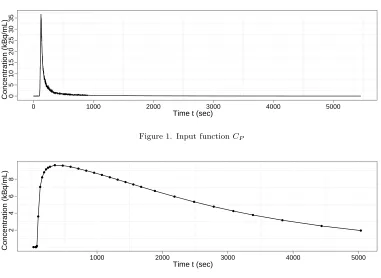
input function, taken from [28], is used (see Figure 1). The simulated data has 32 time frames with lengths corresponding to the integration periods used in real experiments (27.5, 32.5, 2×10, 20, 6×30, 75, 11×120, 210, 5×300, 450, and 2_×600, all in seconds), see Figure 2 for the synthetic noise free data. Noise is added to the synthetic data such that the noise is normally-distributed with mean zero, and variance proportional to the time activities divided by the length of time frames. The noise is scaled such that the highest variance in the sequence is equal to a “noise level” variable (with the others scaled in proportion). This noise level ranges from 0.01 to 5.12, from lower than typical region of interest (ROI) analysis (in which the data is averaged over a biologically meaningful region in order to improve signal to noise ratio) to higher than the noise associated with voxel-level analysis [38]. For each noise level, 2,000 time series were simulated. Normally-distributed errors were assumed (correctly, in this simulation study). For each of these time series analysis was carried out for each of the three possible models via likelihood-based and Bayesian methods as detailed previously.

The NLS procedures use thedirectalgorithm [30] to find a local minimum, and

then uses this minimum to initialise a Nelder-Mead simplex algorithm [36]. The programs used for both likelihood-based and Bayesian modeling are implemented in C++ [45] and are available from the first author on request.

Time t (sec)

Concentr

ation (kBq/mL)

0

5

10

15

20

25

30

35

0 1000 2000 3000 4000 5000

Figure 1. Input functionCP

Time t (sec)

Concentr

ation (kBq/mL)

2

4

6

8

1000 2000 3000 4000 5000

Figure 2. Noise free simulated data

Table 1. MSE ofV_D, three-compartment model

Noise level

Method 0.01 0.02 0.04 0.08 0.16 0.32 0.64 1.28 2.56 5.12

NLS 0.00050.001 0.004 0.017 0.032 0.052 0.103 0.221 0.572 1.191 Bayesian vague 0.00050.00090.002 0.004 0.008 0.015 0.031 0.053 0.105 0.207 Bayesian informative 0.00040.00080.002 0.003 0.007 0.013 0.027 0.052 0.104 0.195

the three-compartment model, obtained by NLS, and also by Bayesian estimation with vague and informative priors. As shown in the table, the NLS estimates are good at low noise level. But at the noise levels typically observed in voxel-level analyses, the Bayesian estimates have significantly smaller MSE. The estimates obtained using informative priors improve at low noise level and are comparable to the estimates with uniform priors at high noise level. In general the Bayesian estimates are more stable than the NLS estimates, which is known to have positive bias that increases with noise level [38].

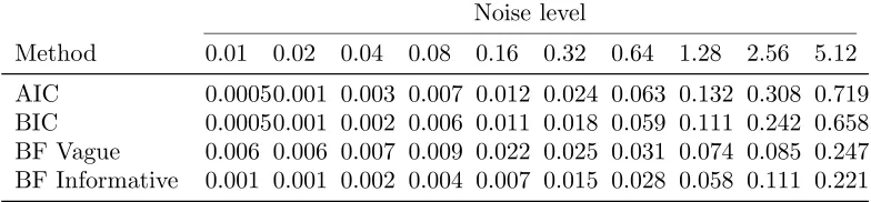
Model selection Tables 2 and 3 summarise the proportion of times each order of model is selected by the information criteria techniques and by choosing the a posteriori most probable model with a uniform prior over model order, respectively. Table 4 summarises the MSE of estimates using selected model under these model selection strategy. As shown in the table, both the frequency with which the true model is chosen and the MSE of estimated for selected models are improved by using Bayesian model selection. Model selection is improved, particularly at higher noise levels, by the use of informative priors. However, in all cases, the true model is hard to identify due to the limited temporal data, even at low noise levels.

Table 2. Frequencies of model selected by AIC and BIC (%)

Noise level

Model 0.01 0.02 0.04 0.08 0.16 0.32 0.64 1.28 2.56 5.12

AIC 1 0 0.1 0.6 1.0 1.8 16.3 48.8 78.3 91.6 98.5 2 91.6 94.0 95.0 96.3 96.6 83.1 50.7 21.5 8.3 2.5

3 8.4 5.9 4.4 2.7 1.6 0.6 0.5 0.2 0.1 0

BIC 1 0 0.1 0.8 1.3 3.5 27.1 64.9 87.8 95.7 98.6 2 94.6 96.2 96.1 96.8 95.5 72.7 35.0 12.2 4.3 1.4

3 5.4 3.7 3.1 1.9 1.0 0.2 0.1 0 0 0

Table 3. Frequencies of model selected by Bayes factors (with vague and informative priors) (%)

Noise level

Model 0.01 0.02 0.04 0.08 0.16 0.32 0.64 1.28 2.56 5.12

Vague 1 0 0 0 0 6.3 7.0 24.3 30.7 41.6 54.8

Priors 2 12.5 20.1 35.2 49.4 55.3 67.5 62.6 59.1 52.2 43.0 3 87.5 79.9 64.8 50.6 38.4 25.5 13.1 10.2 6.2 2.2

Informative 1 0 0 0 0 0 1.0 6.2 15.2 27.8 37.1

Priors 2 10.6 17.5 33.3 45.8 58.8 70.2 73.0 67.3 57.3 53.0 3 89.4 82.5 66.7 54.2 41.2 28.8 20.8 17.5 14.9 9.9

Table 4. MSE ofV_D, selected model

Noise level

Method 0.01 0.02 0.04 0.08 0.16 0.32 0.64 1.28 2.56 5.12

AIC 0.00050.001 0.003 0.007 0.012 0.024 0.063 0.132 0.308 0.719 BIC 0.00050.001 0.002 0.006 0.011 0.018 0.059 0.111 0.242 0.658 BF Vague 0.006 0.006 0.007 0.009 0.022 0.025 0.031 0.074 0.085 0.247 BF Informative 0.001 0.001 0.002 0.004 0.007 0.015 0.028 0.058 0.111 0.221

4.2 Measured [11_{C]diprenorphine data}

Having verified that the proposed method is effective when applied to data sim-ulated from the model, we turn our attention to real data sets which have been considered in the literature using this model.

Data from the a PET study using [11_{C]diprenorphine are used to examine the}

methods presented. The overall aim of the study was to quantify opioid receptor concentration in the brain of normal subjects allowing a baseline to be found for subsequent studies on diseases such as epilepsy. Diseases such as epilepsy tend to involve changes in brain receptor concentrations or occupancy levels either due to physical lesions within the brain or other chemically relevant differences from normal controls. The data have been previously analysed in [38] and in [28] but in both these previous analyses, parameter estimation rather than model com-parison was the focus. Two dynamic scans from a measured [11C]diprenorphine study of normal subjects, for which an arterial input function was available, were analysed. [11C]diprenorphine is a tracer that binds to the opioid (pain) receptor system in the brain. The subjects underwent 95-min dynamic [11C]diprenorphine PET baseline scans on the same camera. The subjects were injected 185 MBq of [11C]diprenorphine. PET scans were acquired in 3D mode on a Siemens/CTI ECAT EXACT3D PET camera, with a spatial resolution after image reconstruction of ap-proximately 5mm. Data were reconstructed using the reprojection algorithm [32] with ramp and Colsher filters cutoff at the Nyquist frequency. Reconstructed voxel size were 2.096mm ×2.096mm ×2.43mm. Acquisition was performed in listmode (event-by-event) and scans were rebinned into 32 time frames of increasing du-ration. Frame-by-frame movement correction was performed on the PET images. Overall this resulted in images of size 128 ×128 ×95 voxels, which when masked to include only brain regions, resulted, for the two data sets analysed below, in 233,054 and 250,570 separate time series respectively to be analysed. Thus this represents a massive repeated application of the proposed framework for Bayesian analysis.

Nonnegative least squares (NNLS) estimates ofVD [9] are available from a

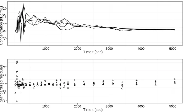
previ-ous study for both data sets and are used as a baseline for comparison (NNLS can be used due to the non-negative nature of the underlying rate constants). The AIC and BIC strategies select the model with smallest AIC or BIC, respectively, while the Bayesian strategy selects the model with highest marginal likelihood. The NLS procedures are exactly the same as in the simulation study. One-, two- and three-tissue compartment models are fitted. The same models (with normally-distributed errors) were also subjected to Bayesian analysis. However, the results are not rea-sonable. Figure 3 shows the time series associated with five typical voxels and their standardised residuals (which in the case of a normal error model should have a standard normal distribution). The NNLS estimates for these five voxels are all around 25 or above. But the Bayesian estimates with normally-distributed errors are about 15. In fact, for most voxels, the Bayesian estimates are about 50% smaller than the NNLS estimates. This can be explained by noting that for the first three data observations, the input function is nearly zero. Hence whatever values of pa-rameters are proposed, the fitted value of CT(t) will be near zero for these three

order to mitigate against this effect: this ad hoc procedure is essential in order to obtain reasonable results with this model.

As shown in the figure, all of the five typical voxels have large residuals at the start of the time-activity course. With normally-distributed errors, these points will have very small probability. Testing the residuals against normal distribution with Kolmogorov-Smirnov test (which is overly conservative as the parameters of the normal distribution have been estimated) shows that for the great majority of the voxels across the whole space, the null hypothesis (that residuals are from a normal distribution) should be rejected at a 5% level. A possible solution to this problem is proposed here. The t distribution is used in place of the normal distribution to model the errors. The t distribution can have a heavy tail and is more robust to outliers than the normal distribution. As shown in figure 3, the data residuals demonstrate rather systematic and substantial departures from the normal distributions.

Time t (sec)

Concentr

ation (kBq/mL)

−5

0

5

10

15

1000 2000 3000 4000 5000

Time t (sec)

Standardiz

ed residuals

−4

−2

0

2

4

1000 2000 3000 4000 5000

Figure 3. Measured CT(t) for five typical voxels and their standardized residuals, fitted with NLS for three-compartments models

For these reasons, we propose using a more heavily-tailed t distribution to model error structures for Bayesian inference. It is natural to use Bayes factor to compare the normal andt-distributed error models. For the five typical data sets in Figure 3, we fitted the three compartment model with both noise distributions and computed the marginal likelihood. For each data set and model, 1,000 repetitions were carried out to quantify the Monte Carlo error. Table 5 compares the logarithm of the marginal likelihood for these data. It is seen that the t-distributed error model is far more plausible from a Bayesian perspective. In addition, this model indeed gave reasonable estimates for the parameter of interest VD

Table 5. Bayesian model comparison between Normal andt-distributed errors

Model Logarithm of marginal likelihood (standard derivation)

Normal -145 (_±1.2) -147 (_±1.1) -138 (_±1.3) -141 (_±0.9) -132 (_±1.1) t -75 (±0.6) -77 (±0.8) -69 (±0.7) -70 (±0.4) -64 (±0.9)

recognise that simple diagnostics do not guarantee that an MCMC algorithm is sufficiently fast mixing, they can at least show evidence that a chain has not converged. It is self-evident that the absence of evidence of non-convergence is a minimal requirement for the output of an MCMC algorithm to be trusted.

For each time series, 100,000 iterations were used for burn-in and a further 100,000 iterations are used to make the subsequent inference. The estimates of

VD and the marginal likelihood p(D) are the primary objects of inference. In order

to assess the convergence, the MCMC chain was initialised with dispersed starting values. Figure 6 shows the estimates of VD from the burn-in iterations of a typical

voxel when starting the chain from different values. As shown in the plot, 40,000 iterations is enough for the chain to mix well and get a good estimate for VD,

the parameter of interest, as mentioned above, 100,000 samples were used for a conservative burn-in period. Similar plots were produced for other parameters and they all showed that chains initialized from different areas of the parameter space produce very similar estimates. It is, of course, not feasible to manually inspect such traces for all voxels, however 200 voxels with a range of values of VDs were

examined in this way. It was found that the algorithm mixed well for voxels from different regions of the brain.

A more quantitative technique was employed to check for evidence of poor mixing throughout the (1.5 million) chains used in the real-data examples. Following [15], the variance of the estimate of VD obtained from the final 10,000 samples of the

chain was divided by that of the estimate ofVD obtained by all post-burn-in samples

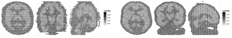
(100,000); a value of between 0.9 and 1.1 is recommended as an indication that the chain has reached stationarity (for a single simulation run) by [15]. In our case, we consider a summary of the 1.5 million chains used to describe the large number of voxels in the brain under several modeling regimes and we found that this ratio was between 0.9 and 1.1 for 91.2% of all voxels. Figure 4 shows that for both data sets, the ratio is universally within the 0.7 to 1.2 interval. The actual variance of estimate ofVD from Bayesian estimation for the two data sets is shown in Figure 5.

In addition, much longer chains were run to examine the behavior of the algo-rithm. Table 6 shows the estimates of a typical voxel when using different length of the MCMC chain. As seen in the table, with long chains, the estimates does not change substantially suggesting that the algorithm has converged to stationarity for even the shortest chains (of course, no such diagnostic provides proof that this is the case, but these are the type of diagnostics most routinely used).

Ratio (0.7,0.8] (0.8,0.9] (0.9,1] (1,1.1] (1.1,1.2]

Ratio (0.7,0.8] (0.8,0.9] (0.9,1] (1,1.1] (1.1,1.2]

Figure 4. Convergence Diagnostic: ratio of variance of final 10,000 samples to that of full 100,000 samples

0.02 0.03 0.04 0.05

var(VD)

0.02 0.03 0.04 0.05

var(VD)

Iterations

P

oster

ior mean of VD

10

15

20

25

30

2e+04 4e+04 6e+04 8e+04 1e+05

Figure 6. Cumulative sample averages ofVDwhen starting the MCMC chain from different values for a typical voxel

Table 6. Estimates from a long chain for a typical voxel

Chain lengths

Parameter 104 _5×104 ₁₀5 _5×105 ₁₀6 _2×106

VD 25.71 25.67 25.64 25.75 25.82 25.73

p(D)/10−31 _{3.22 3.45 3.36 3.23 3.31 3.39}

EstimationFigure 7 shows the estimates ofVD for a three-compartments model,

using Bayesian posterior means with informative priors and NLS, together with the NNLS estimates obtained by [28] for the data. Overall the percentage difference between NNLS and NLS ((NNLS - NLS) / NLS) is about 3%. This difference is fairly uniform overall the range of VD, though there are large percentage

differ-ence for voxels with very small values of VD. This is due to the fact that different

bounds/priors are applied to the space of theφandθparameters and different esti-mates are obtained when the value of parameters are near the boundaries. However, these voxels are less of interest as they correspond to regions with little or no ac-tivity and hence little receptor density. The Bayesian estimates are roughly 5% smaller than the NNLS estimates. Previous studies showed that NNLS has about 5% positive bias with noise levels typical of a voxel analysis [38]. There are similar large differences for voxels with small VD as with the NLS estimates. Overall, if

we take the results of previous simulation study of NNLS, then the Bayesian esti-mates would appear to offer better estimation than NNLS estiesti-mates. In addition, a principled way of introducing the prior knowledge concerning the rate constants has been used and a more appropriate noise model has been employed aiding inter-pretation of the results. Similar results were obtained for both [11C]diprenorphine scans indicating somewhat reproducible results (Figure 8).

As implemented on a 3.07GHz Xeon processor, the average (single core) CPU time per voxel is 0.15 seconds for the MCMC algorithm. Using a fairly standard 4-core CPU system, this equates to approximately two hours for a complete PET scan. While significantly longer than the equivalent NNLS implementation (approx-imately 5 minutes on a similar system), we do not believe that this is prohibitively slow, even for routine analysis, particularly given the additional information and accuracy achieved. Furthermore, the length of chain employed in this study has been rather conservative and a significant increase in speed could be achieved with very little reduction in estimation accuracy.

on [11_{C]diprenorphine have shown that finding a particular single compartmental}

structure for the entire brain is unrealistic [22]. However, the model selection results of AIC and BIC do not exhibit any obvious spatial structure. For both, the two-compartment model is most widely favored. When using Bayesian model selection, the one-compartment model dominates in low activity areas. These areas are of less interest, but the findings are perhaps interesting. Identifying the parameters of a second or third compartment in areas with barely any activity is rather difficult. In the extreme case, for a voxel with no activity but noisy signals, the model can have arbitrary compartments, each of them having near zero concentration. Using Bayesian model comparison, the one-compartment model is chosen which at least favors a parsimonious representation; it could be argued that a null model should be added to the class of models under consideration to account for this case.

Within the areas of greatest interest in which a real neurological signal is ex-pected, the two-compartment model is favored most often. However, there are more three-compartments model selected in high VD areas. Overall the image of

model order for the Bayesian analysis shows rather more spatial structure than the AIC and BIC cases although none has been imposed. It is biologically reasonable to believe that there are similar compartmental structures for voxels within the same area and different compartmental structures for voxels from different regions. Although we don’t know what the true model is, or indeed believe that there is a true compartmental model in this setting, the Bayesian model selection, which reveals spatial structure, is more convincing than the other two. Indeed methods that do not require the specification of a single compartmental structure for the whole brain are well known to be preferred when modeling [11_{C]diprenorphine [22].}

The different model structures can also be quantified and uncertainty attached to the estimates of the model order. Also shown in Figures 7 and 8 are the posterior model probabilities of the chosen model. For the majority of the voxels, the chosen model has a posterior probabilityp(M|D)≥0.5. For lowVD regions, the posterior

probability is much higher indicating that there is relatively high confidence that one compartment is adequate to explain what is observed in these regions but that there is a lack of strong evidence to support a particular model configuration in the case of more active regions.

Overall, the Bayesian model selection framework provides comparable parameter estimation performance with other methods such as those in [38] and [28], empiri-cally alleviating the biases associated with NNLS, but in addition yields evidence as to the posterior probability of the chosen models. This gives valuable additional information when analysing subsequent normal or patient data. Regions where there is considerable uncertainty will require larger deviations in patient popula-tions to establish differences, thus helping inform study designs in applicapopula-tions with tracers such as [11C]diprenorphine. In addition, Bayesian model averaging can be performed trivially using the output from the MCMC analysis.

5. Conclusions

The purpose of this paper is not to advocate a particular computational approach to Bayesian model selection but to show the potential gains associated with adopt-ing a Bayesian approach to the problem in the context of PET studies in particular. It is, of course, possible to employ other computational algorithms to perform pa-rameter estimation and model selection jointly within a simulation run, employing RJMCMC [19], for example. In more complex problems these approaches may be more appropriate; the simple approach adopted here was adequate for the studies that we have encountered thus far and we would anticipate will be so for other PET compartmental studies of this type. The theoretical concerns that have been raised about the method of [13] are not a consideration in the present context as it is easy to control the relative tail behavior of the target and the “importance density” thereby ensuring that this quantity is bounded and does not lead to in-finite variance. Although much recent work has focused on samplers that explore all models simultaneously, it is not clear that such a strategy is always preferable. Indeed, to quote from [23]:

“. . . there is no one answer, and in some instances trans-dimensional moves will help samplers, whereas in others they will be unnecessary.”

Furthermore, preliminary work investigating more sophisticated algorithms for the calculation of model evidence [50] has shown very close agreement between a novel Sequential Monte Carlo algorithm based upon path-sampling [14] and the sim-ple approach developed here (although greater computational efficiency can be obtained with more sophisticated machinery). Ongoing work is investigating the performance improvements that can be obtained by such methods.

We have demonstrated that the most widely used model does not fit real PET data well and proposed a simple extension using a t-distributed noise model. This allows for the direct estimation of models even when moderate outliers are present in the data. This is very often the case with real data, for example, the delay of the input into the system is often not constant for all locations. In addition, calculating uncertainty estimates for both models and estimates are possible, something which it is inherently difficult (if not impossible) to achieve with methods based around NNLS and other point estimation techniques. This provides considerable additional information when comparing scans, and will be of particular interest when com-paring normal controls verses patient groups where lesions or other pathological problems may introduce considerable differences in the uncertainty of the measures for different scans.

It would be interesting to develop methods to exploit spatial homogeneity within the brain to improve performance and produce more parsimonious inference. Fur-ther investigation into the modeling problem may also be warranted as the above demonstrate that the assumption of normally-distributed errors is not consistent with real data and with a heavier-tailed noise distribution it is not possible to obtain strong evidence in support of any one model using the type of data which is typically available. With the present modeling approach, macro parameters and other such quantities of interest could be more robustly estimated by Bayesian model averaging than by any approach based upon model selection (see, for exam-ple, [6], Chapter 6) and that is the strategy that we would recommend.

References

[1] S. Brooks, A. Gelman, G.L. Jones, and X.L. Meng (eds.), CRC Press 2011. [2] H. Akaike, Information theory and an extention of the maximum likelihood

USA, 1973, pp. 610–624.

[3] N.M. Alpert and F. Yuan,A general method of Bayesian estimation for para-metric imaging of the brain, Neuroimage 45 (2009), pp. 1183–1189.

[4] D.H. Anderson, Lecture Notes in Biomathematics, Vol. 50, Springer-Verlag, New York, USA 1983.

[5] J.A.D. Aston, R.N. Gunn, K.J. Worsley, Y. Ma, A.C. Evans, and A. Dagher,

A statistical method for the analysis of positron emission tomography neurore-ceptor ligand data, Neuroimage 12 (2000), pp. 245–256.

[6] J.M. Bernardo and A.F.M. Smith, John Wiley & Sons, Chichester, UK 2000. [7] N. Chopin and C.P. Robert, Comments on “Estimating the integrated likeli-hood via posterior simulation using the harmonic mean identity” by Raftery et al., in Bayesian Statistics 8, J.M. Bernardo, M.J. Bayarri, J.O. Berger, A.P. Dawid, D. Heckerman, A.F.M. Smith, and M. West, eds., Oxford University Press, 2007, pp. 40–41.

[8] P. Congdon, 3rd ed., John Wiley & Sons, West Sussex, UK 2006.

[9] V.J. Cunningham and T. Jones, Spectral analysis of dynamic PET studies, Journal of Cerebral Blood Flow and Metabolism 13 (1993), pp. 15–23. [10] P. Del Moral, A. Doucet, and A. Jasra, Sequential Monte Carlo samplers,

Journal of the Royal Statistical Society B 63 (2006), pp. 411–436.

[11] W.G. Frankle and M. Laruelle,Neuroreceptor imaging in psychiatric disorders, Annals of Nuclear Medicine 16 (2002), pp. 437–46.

[12] S.S. Gambhir,Molecular imaging of cancer with positron emission tomography, Nature Reviews Cancer 2 (2002), pp. 683–693.

[13] A.E. Gelfand and D.K. Dey, Bayesian model choice: asymptotics and exact calculations, Journal of the Royal Statistical Society. Se-ries B (Statistical Methodology) 56 (1994), pp. 501 – 514, URL http://www.jstor.org/stable/2346123.

[14] A. Gelman and X.L. Meng, Simulating normalizing constants: From impor-tance sampling to bridge sampling to path sampling, Statistical Science 13 (1998), pp. 163–185.

[15] A. Gelman and K. Shirley, Inference from simulations and monitoring con-vergence, in Brooks et al. [1], pp. 163–174.

[16] A. Gelman, J.B. Carlin, H.S. Stern, and D.B. Rubin, Chapman & Hall/CRC 2004.

[17] J. Geweke, Bayesian inference in econometric models using Monte Carlo in-tegration, Econometrica: Journal of the Econometric Society 57 (1989), pp. 1317–1339, URL http://www.jstor.org/stable/1913710.

[18] G. Gibson and E. Renshaw,Estimating parameters in stochsatic compartmen-tal models using Markov chain methods, IMA Journal of Mathematics Applied in Medicine and Biology 15 (1998), pp. 19–40.

[19] P.J. Green, Reversible jump Markov Chain Monte Carlo computation and Bayesian model determination, Biometrika 82 (1995), pp. 711–732.

[20] P.J. Green, Trans-dimensional Markov chain Monte Carlo, in Highly Struc-tured Stochastic Systems, P.J. Green, N.L. Hjort, and S. Richardson, eds., chap. 6, Oxford University Press, 2003, pp. 179–206.

[21] R.N. Gunn, S.R. Gunn, and V.J. Cunningham, Positron emission tomogra-phy compartmental models, Journal of Cerebral Blood Flow & Metabolism 21 (2001), pp. 635–52, URLhttp://www.ncbi.nlm.nih.gov/pubmed/11488533. [22] A. Hammers, M.C. Asselin, F.E. Turkheimer, R. Hinz, S. Osman, G. Hotton,

http://www.sciencedirect.com/science/article/pii/S1053811907005745. [23] D. Hastie and P.J. Green, Model choice using reversible jump Markov chain

Monte Carlo, Statistica Neerlandica (2012), to appear.

[24] R.A. Hawkins, M.E. Phelps, and S.C. Huang, Effects of temporal sampling, glucose metabolic rates, and disruptions of the blood-brain barrier on the FDG model with and without a vascular compartment: studies in human brain tu-mors with PET, Journal of Cerebral Blood Flow & Metabolism 6 (1986), pp. 170–183, URLhttp://dx.doi.org/10.1038/jcbfm.1986.30.

[25] C.M. Hurvich and C.L. Tsai, Regression and time series model se-lection in small samples, Biometrika 76 (1989), pp. 297–307, URL http://biomet.oxfordjournals.org/cgi/content/abstract/76/2/297. [26] R.B. Innis, V.J. Cunningham, J. Delforge, M. Fujita, R.N. Gunn, J. Holden,

S. Houle, S.C. Huang, M. Ichise, H. Iida, H. Ito, Y. Kimura, R.A. Koeppe, G.M. Knudsen, J. Knuuti, A.A. Lammertsma, M. Laruelle, R.P. Maguire, M. Mintun, E.D. Morris, R. Parsey, J. Price, M. Slifstein, V. Sossi, T. Suhara, J. Votaw, D.F. Wong, and R.E. Carson, Consensus nomenclature for in vivo imaging of reversibly binding radioligands, Journal of Cerebral Blood Flow and Metabolism 27 (2007), pp. 1533–1539.

[27] J.A. Jacquez, 3rd ed., University of Michigan Press 1996.

[28] C.R. Jiang, J.A.D. Aston, and J.L. Wang, Smoothing dynamic

positron emission tomography time courses using functional

prin-cipal components, NeuroImage 47 (2009), pp. 184–93, URL

http://www.ncbi.nlm.nih.gov/pubmed/19344774.

[29] A.M. Johansen, P. Del Moral, and A. Doucet,Sequential Monte Carlo samplers for rare events, in Proceedings of the 6th International Workshop on Rare Event Simulation, October, Bamberg, Germany, 2006, pp. 256–267.

[30] D.R. Jones, C.D. Perttunen, and B.E. Stuckman, Lipschitzian optimization without the Lipschitz constant, Journal of Optimization Theory and Applica-tions 79 (1993), pp. 157–181.

[31] R.E. Kass and A.E. Raftery, Bayes factors, Journal of the American Statistical Association 90 (1995), pp. 773–795, URL http://www.jstor.org/stable/2291091.

[32] P. Kinahan and J. Rogers,Analytic 3D image reconstruction using all detected events, IEEE Transactions on Nuclear Science 36 (1989), pp. 964–968, URL

http://0-ieeexplore.ieee.org.pugwash.lib.warwick.ac.uk/xpls/abs all.jsp?arnumber=34585. [33] A.A. Lammertsma and S.P. Hume, Simplified reference tissue model for PET

receptor studies, Neuroimage 4 (1996), pp. 153–8.

[34] D.J. Lawson, G. Holtrop, and H. Flint, Bayesian analysis of non-linear dif-ferential equation models with application to a gut microbial ecosystem, Bio-metrical Journal 53 (2011), pp. 543–556.

[35] D.A. Mankoff, A.F. Shields, M.M. Graham, J.M. Link, J.F. Eary, and K.A. Krohn, Kinetic analysis of 2-[Carbon-11]Thymidine PET

imaging studies: Compartmental model and mathematical analysis,

The Journal of Nuclear Medicine 39 (1998), pp. 1043–1055, URL http://jnm.snmjournals.org/cgi/content/abstract/39/6/1043.

[36] J.A. Nelder and R. Mead, A simplex method for function

min-imization, The Computer Journal 7 (1965), pp. 308–313, URL

http://comjnl.oxfordjournals.org/cgi/content/abstract/7/4/308. [37] M.A. Newton and A.E. Raftery, Approximate Bayesian inference with

[38] J.Y. Peng, J.A.D. Aston, R.N. Gunn, C.Y. Liou, and J. Ashburner,Dynamic positron emission tomography data-driven analysis using sparse Bayesian learning, IEEE Transactions on Medical Imaging 27 (2008), pp. 1356–69, URL http://www.ncbi.nlm.nih.gov/pubmed/18753048.

[39] M.E. Phelps, Positron emission tomography provides

molecular imaging of biological processes (2000), URL

http://www.pnas.org/cgi/doi/10.1073/pnas.97.16.9226.

[40] A.E. Raftery, M.A. Newton, J. Satagopan, and P. Krivitsky, Estimating the integrated likelihood via posterior simulation using the harmonic mean identity (with discussion), in Bayesian Statistics 8, J.M. Bernardo, M.J. Bayarri, J.O. Berger, A.P. Dawid, D. Heckerman, A.F.M. Smith, and M. West, eds., Oxford University Press, 2007, pp. 1–45.

[41] C.P. Robert, 2nd ed., Springer, New York, USA 2007.

[42] C.P. Robert and G. Casella, 2nd ed., Springer, New York, USA 2004.

[43] K. Schmidt, Which linear compartmental systems can be analyzed by spec-tral analysis of PET output data summed over all compartments?, Journal of Cerebral Blood Flow & Metabolism 19 (1999), pp. 560–9.

[44] G. Schwarz, Estimating the dimension of a model, The Annals of Statistics 6 (1978), pp. 461 – 464, URL http://www.jstor.org/stable/2958889. [45] B. Stroustrup, 2nd ed., Addison Wesley 1991.

[46] L. Tierney, Markov chains for exploring posterior

distribu-tions, The Annals of Statistics 22 (1994), pp. 1701–1728, URL

http://www.jstor.org/stable/2242477.

[47] F.E. Turkheimer, R. Hinz, and V.J. Cunningham, On the undecidabil-ity among kinetic models: From model selection to model averaging, Jour-nal of Cerebral Blood Flow & Metabolism 23 (2003), pp. 490–498, URL http://dx.doi.org/10.1097/01.WCB.0000050065.57184.BB.

[48] F.E. Turkheimer, J.A.D. Aston, M.C. Asselin, and R. Hinz, Multi–resolution Bayesian regression in PET dynamic studies using wavelets, Neuroimage 32 (2006), pp. 111–121.

[49] J. Wakefield, The Bayesian analysis of population pharmacokinetic models, Journal of the American Statistical Association 91 (1996), pp. 62–75.

0 , 2 0 1 3 J o u rn a l o f A p p lie d S ta ti st ic s p a p er -c J A S 2 e R E F E R E N C E S 2 5 NNLS VD 7 10 13 16 19 22 25 28 31 34 37 NLS VD 7 10 13 16 19 22 25 28 31 34 37 Bayesian VD 7 10 13 16 19 22 25 28 31 34 37

Bayesian model averaging

VD 7 10 13 16 19 22 25 28 31 34 37 AIC Model order 1 2 3 BIC Model order 1 2 3 Bayes factor Model order 1 2 3

Posterior model probabilities

Model prob. 0.0 0.1 0.2 0.3 0.4 0.5 0.6 0.7 0.8 0.9 1.0

0 , 2 0 1 3 J o u rn a l o f A p p lie d S ta ti st ic s p a p er -c J A S 2 e 2 6 R E F E R E N C E S NNLS VD 10 13 16 19 22 25 28 31 34 37 40 NLS VD 10 13 16 19 22 25 28 31 34 37 40 Bayesian VD 10 13 16 19 22 25 28 31 34 37 40

Bayesian model averaging

VD 10 13 16 19 22 25 28 31 34 37 40 AIC Model order 1 2 3 BIC Model order 1 2 3 Bayes factor Model order 1 2 3

Posterior model probabilities

Model prob. 0.0 0.1 0.2 0.3 0.4 0.5 0.6 0.7 0.8 0.9 1.0